Vol. 4, No. 4, Year 2012 Article ID IJIM-00299, 16 pages Research Article
Application of Iterative Methods for Solving
General Riccati Equation
T. Allahviranlooa, Sh. S. Behzadib ∗
(a)Department of Mathematics, Islamic Azad University, Central Tehran Branch, Tehran, Iran. (b)Department of Mathematics, Islamic Azad University, Qazvin Branch, Qazvin, Iran.
——————————————————————————————————
Abstract
In this paper, the general Riccati differential equation is solved by using the Adomian’s decomposition method (ADM) , modified Adomian’s decomposition method (MADM), variational iteration method (VIM), modified variational iteration method (MVIM), ho-motopy perturbation method (HPM), modified hoho-motopy perturbation method (MHPM) and homotopy analysis method (HAM). The existence and uniqueness of the solution and convergence of the proposed methods are proved in details. A numerical example is stud-ied to demonstrate the accuracy of the presented methods.
Keywords: General Riccati equation; Adomian decomposition method; Modified Adomian decom-position method; Variational iteration method; Modified variational iteration method; Homotopy perturbation method; Modified homotopy perturbation method; Homotopy analysis method. ——————————————————————————————————
1
Introduction
The Riccati differential equation is named after the Italian nobleman Count Jacopo Francesco Riccati (1676-1754). The book of Reid [1] contains the fundamental theories of Riccati equation, with applications to random processes, optimal control, and diffusion problems. Besides important engineering science applications that today are considered classical, such as stochastic realization theory, optimal control, robust stabilization, and network synthesis, the newer applications include such areas as financial mathematics [2, 3]. In recent years some works have been done in order to find the numerical solution of this equation, for example [4, 5, 6, 7, 8, 9]. In this work, we develope the ADM, MADM, VIM, MVIM, HPM, MHPM and HAM to solve the general Riccati differential equation as follows:
ut=Q(t)u+R(t)u2+P(t), (1.1)
∗Corresponding author. Email address: shadan [email protected].
with the initial condition:
u(0) =g(t). (1.2)
Where Q(t), R(t), P(t) and g(t) are scalar functions.
The paper is organized as follows. In Section 2, the mentioned iterative methods are introduced for solving Eq.(1.1). In Section 3 we prove the existence and uniqueness of the solution and convergence of the proposed methods. Finally, the numerical example is shown in Section 4.
In order to obtain an approximate solution of Eq.(1.1) and Eq.(1.2), let us integrate one time Eq.(1.1) with respect tot using the initial condition we obtain,
u(t) =F(t) + ∫ t
0
F1(u(s))ds+
∫ t
0
F2(u(s)) ds, (1.3)
where,
F(t) =g(t) +∫0tP(s) ds, F1(u(t)) =Q(t)u(t),
F2(u(x, t)) =R(t)u2(t).
In Eq.(1.3), we assumeF(t) is bounded for all tinJ = [0, T](T ∈R).
The termsF1(u(x, t)) andF2(u(x, t)) are Lipschitz continuous with|F1(u)−F1(u∗)|≤
L1 |u−u∗ |and|F2(u)−F2(u∗)|≤L2 |u−u∗ |.
2
The iterative methods
2.1 Description of the MADM and ADM
The Adomian decomposition method is applied to the following general nonlinear equation
Lu+Ru+N u=g1, (2.4)
where u(t) is the unknown function, L is the highest order derivative operator which is assumed to be easily invertible,R is a linear differential operator of order less thanL, N u represents the nonlinear terms, and g1 is the source term. Applying the inverse operator
L−1 to both sides of Eq.(1.3), and using the given conditions we obtain
u(t) =f1(t)−L−1(Ru)−L−1(N u), (2.5)
where the functionf1(t) represents the terms arising from integrating the source term g1.
The nonlinear operator N u=G1(u) is decomposed as
G1(u) =
∞
∑
n=0
An, (2.6)
where An, n≥0 are the Adomian polynomials determined formally as follows :
An=
1 n![
dn dλn[N(
∞
∑
i=0
The first Adomian polynomials (introduced in [10, 11, 12]) are:
A0 =G1(u0),
A1 =u1G′1(u0),
A2 =u2G′1(u0) +
1 2!u
2
1G′′1(u0), (2.8)
A3 =u3G′1(u0) +u1u2G′′1(u0) +
1 3!u
3
1G′′′1(u0), ...
2.1.1 Adomian decomposition method
The standard decomposition technique represents the solution of u(t) in Eq.(2.4) as the following series,
u(t) =
∞
∑
i=0
ui(t), (2.9)
where, the componentsu0, u1, . . . which can be determined recursively
u0(t) =F(t),
u1(t) =
∫ t
0
A0(s) ds+
∫ t
0
B0(s) ds,
.. .
un+1(t) =
∫ t
0
An(s) ds+
∫ t
0
Bn(s)ds, n≥0. (2.10)
Substituting Eq.(2.8) into Eq.(2.10) leads to the determination of the components of u(t).
2.1.2 The modified Adomian decomposition method
The modified decomposition method was introduced by Wazwaz [13]. The modified forms was established on the assumption that the function F(t) can be divided into two parts, namely f1(t) and f2(t). Under this assumption we set
F(t) =f1(t) +f2(t). (2.11)
Accordingly, a slight variation was proposed only on the componentsu0(t) andu1(t). The
suggestion was that only the partf1 be assigned to the zeroth componentu0(t), whereas
the remaining partf2 be combined with the other terms given in Eq.(2.11) to defineu1(t).
Consequently, the modified recursive relation
u0(t) =f1(t),
u1(t) =f2(t)−L−1(Ru0)−L−1(A0), (2.12)
.. .
un+1(t) =−L−1(Run)−L−1(An), n≥1,
To obtain the approximation solution of Eq.(1.1), according to the MADM, we can write the iterative formula Eq.(2.12) as follows:
u0(t) =f1(t),
u1(t) =f2(t) +
∫t
0 A0(s) ds+
∫t
0B0(s)ds,
.. .
un+1(t) =
∫t
0 An(s) ds+
∫t
0Bn(s) ds, n≥1.
(2.13)
The operators F1(u(t)) and F2(u(t)) are usually represented by the infinite series of
the Adomian polynomials as follows:
F1(u(t)) =
∞
∑
i=0
Ai(t),
F2(u(t)) =
∞
∑
i=0
Bi(t),
whereAi and Bi are the Adomian polynomials.
Also, we can use the following formula for the Adomian polynomials [14]:
An =F1(sn)−
∑n−1
i=0 Ai,
Bn=F2(sn)−
∑n−1
i=0 Bi.
(2.14)
Wheresn=
∑n
i=0ui(t) is the partial sum.
2.2 Description of the VIM and MVIM
In the VIM [14, 15, 16, 17, 18], it has been considered the following nonlinear differential equation:
Lu+N u=g1, (2.15)
where L is a linear operator, N is a nonlinear operator and g1 is a known analytical
function. In this case, the functions un may be determined recursively by
un+1(t) =un(t) +
∫ t
0
λ(τ){L(un(τ)) +N(un(τ))−g1(τ)}dτ, n≥0, (2.16)
whereλis a general Lagrange multiplier which can be computed using the variational the-ory. Here the functionun(τ) is a restricted variations which meansδun= 0. Therefore, we
first determine the Lagrange multiplier λthat will be identified optimally via integration by parts. The successive approximation un(t), n≥ 0 of the solution u(t) will be readily
obtained upon using the obtained Lagrange multiplier and by using any selective function u0(t). The zeroth approximationu0(t) may be selected any function that just satisfies at
least the initial and boundary conditions. Withλdetermined, then several approximation un(t), n ≥ 0 follow immediately. Consequently, the exact solution may be obtained by
using
u(t) = lim
n→∞un(t). (2.17)
To obtain the approximation solution of Eq.(1.1), according to the VIM, we can write Eq.(2.16) as follows:
un+1(t) =un(t) +Lt−1(λ[un(s)−F(s)−
∫t
0(F1(un(s))ds−
∫t
0F2(un(s))ds]), n≥0.
(2.18) Where,
L−t1(.) = ∫ t
0
(.)dτ.
To find the optimalλ, we proceed as
δun+1(t) =δun(t) +δLt−1(λ[un(s)−F(s)−
∫t
0 F1(un(s)) ds−
∫t
0 F2(un(s))ds]).
(2.19) From Eq.(2.19), the stationary conditions can be obtained as follows:
λ′ = 0 and 1 +λ= 0.
Therefore, the Lagrange multipliers can be identified as λ =−1 and by substituting in Eq.(2.18), the following iteration formula is obtained.
u0(t) =F(t),
un+1(t) =un(t)−Lt−1(un(s)−F(s)−
∫t
0F1(un(s))ds−
∫t
0 F2(un(s)) ds), n≥0.
(2.20) To obtain the approximation solution of Eq.(1.1), based on the MVIM [19, 20], we can write the following iteration formula:
u0(t) =F(t),
un+1(t) =un(t)−L−t1(−
∫t
0 F1(un(s)−un−1(s))ds−
∫t
0F2(un(s)−un−1(s))ds), n≥0.
(2.21) Relations Eq.(2.20) and Eq.(2.21) will enable us to determine the components un(t)
recursively for n≥0.
2.3 Description of the HAM
Consider
N[u] = 0,
whereN is a nonlinear operator,u(t) is an unknown function andtis an independent variable. let u0(t) denote an initial guess of the exact solution u(t), h ̸= 0 an auxiliary
parameter, H1(t) ̸= 0 an auxiliary function, and L an auxiliary linear operator with the
property L[s(t)] = 0 whens(t) = 0. Then usingq ∈[0,1] as an embedding parameter, we construct a homotopy as follows:
It should be emphasized that we have great freedom to choose the initial guessu0(t),
the auxiliary linear operator L, the non-zero auxiliary parameter h, and the auxiliary functionH1(t).
Enforcing the homotopy Eq.(2.22) to be zero, i.e.,
ˆ
H1[ϕ(t;q);u0(t), H1(t), h, q] = 0, (2.23)
we have the so-called zero-order deformation equation
(1−q)L[ϕ(t;q)−u0(t)] =qhH1(t)N[ϕ(t;q)]. (2.24)
Whenq = 0, the zero-order deformation Eq.(2.24) becomes
ϕ(t; 0) =u0(t), (2.25)
and when q = 1, since h ̸= 0 and H1(t) ̸= 0, the zero-order deformation Eq.(2.24) is
equivalent to
ϕ(t; 1) =u(t). (2.26)
Thus, according to Eq.(2.25) and Eq.(2.26), as the embedding parameter q increases from 0 to 1, ϕ(t;q) varies continuously from the initial approximation u0(t) to the exact
solution u(t). Such a kind of continuous variation is called deformation in homotopy [20, 21, 22, 23].
Due to Taylor’s theorem, ϕ(t;q) can be expanded in a power series ofq as follows
ϕ(t;q) =u0(t) +
∞
∑
m=1
um(t)qm, (2.27)
where,
um(t) =
1 m!
∂mϕ(t;q) ∂qm |q=0 .
Let the initial guess u0(t), the auxiliary linear parameter L, the nonzero auxiliary
parameterh and the auxiliary function H1(t) be properly chosen so that the power series
Eq.(2.27) ofϕ(t;q) converges atq= 1, then, we have under these assumptions the solution series
u(t) =ϕ(t; 1) =u0(t) +
∞
∑
m=1
um(t). (2.28)
From Eq.(2.28), we can write Eq.(2.25) as follows
(1−q)L[ϕ(t, q)−u0(t)] = (1−q)L[
∑∞
m=1um(t) qm] =q h H1(t)N[ϕ(t, q)]⇒
L[∑∞m=1um(t) qm]−q L[
∑∞
m=1um(t)qm] =q h H1(t)N[ϕ(t, q)]
(2.29)
By differentiating Eq.(2.29)m times with respect toq, we obtain
{L[∑∞m=1um(t) qm]−q L[
∑∞
m=1um(t)qm]}(m)={q h H1(t)N[ϕ(t, q)]}(m)=
m!L[um(t)−um−1(t)] =h H1(t)m ∂
m−1N[ϕ(t;q)]
Therefore,
L[um(t)−χmum−1(t)] =hH1(t)ℜm(um−1(t)), (2.30)
where,
ℜm(um−1(t)) =
1 (m−1)!
∂m−1N[ϕ(t;q)]
∂qm−1 |q=0, (2.31)
and
χm=
{
0, m≤1 1, m >1
Note that the high-order deformation Eq.(2.30) is governing the linear operatorL, and the term ℜm(um−1(t)) can be expressed simply by Eq.(2.31) for any nonlinear operator
N.
To obtain the approximation solution of Eq.(1.1), according to HAM, let
N[u(t)] =u(t)−F(t)−∫0tF1(u(s))ds−
∫t
0F2(u(s))ds,
so,
ℜm(um−1(t)) =um−1(t)−F(t)−
∫t
0F1(um−1(s))ds−
∫t
0F2(um−1(s))ds. (2.32)
Substituting Eq.(2.32) into Eq.(2.30)
L[um(t)−χmum−1(t)] =hH1(t)[um−1(t)−
∫t
0 F1(um−1(s))ds
−∫t
0F2(um−1(s))ds+ (1−χm)F(t)].
(2.33)
We take an initial guessu0(t) =F(t), an auxiliary linear operator Lu=u, a nonzero
auxiliary parameter h = −1, and auxiliary function H1(t) = 1. This is substituted into
Eq.(2.33) to give the recurrence relation
u0(t) =F(t),
un+1(t) =
∫t
0F1(un(s))ds+
∫t
0F2(un(s))ds, n≥0.
(2.34)
Therefore, the solutionu(t) becomes
u(t) =∑∞n=0un(t)
=F(t) +∑∞n=1( ∫0tF1(un(s))ds+
∫t
0F2(un(s))ds
)
. (2.35)
Which is the method of successive approximations. If
|un(t)|<1,
2.4 Description of the HPM and MHPM
To explain HPM [24, 25], we consider the following general nonlinear differential equation:
Lu+N u=f(u), (2.36)
with initial conditions
u(0) =f(t).
According to HPM, we construct a homotopy which satisfies the following relation
H(u, p) =Lu−Lv0+p Lv0+p [N u−f(u)] = 0, (2.37)
where p ∈ [0,1] is an embedding parameter and v0 is an arbitrary initial approximation
satisfying the given initial conditions.
In HPM, the solution of Eq.(2.37) is expressed as
u(t) =u0(t) +p u1(t) +p2 u2(t) +... (2.38)
Hence the approximate solution of Eq.(2.36) can be expressed as a series of the power of p, i.e.
u= lim
p→1u=u0+u1+u2+...
where,
u0(t) =F(t),
.. .
um(t) =
∑m−1
k=0
∫t
0F1(um−k−1(s))ds+
∫t
0F2(um−k−1(s)) ds, m≥1.
(2.39)
To explain MHPM [26, 27, 28, 29], we consider Eq.(1.1) as
L(u) =u(t)−F(t)− ∫ t
0
F1(u(s))ds−
∫ t
0
F2(u(s))ds.
Where F1(u(t)) = g1(t)h1(t) and F2(u(t)) = g2(t)h2(t). We can define homotopy
H(u, p, m) by
H(u,0, m) =f(u), H(u,1, m) =L(u),
where, mis an unknown real number and
f(u(t)) =u(t)−f(t).
Typically we may choose a convex homotopy by
H(u, p, m) = (1−p)f(u) +p L(u) +p (1−p)[m(g1(t) +g2(t))] = 0, 0≤p≤1. (2.40)
Wherem is called the accelerating parameters, and for m= 0 we define H(u, p,0) = H(u, p),which is the standard HPM.
parameterpmonotonically increase from 0 to 1 as trivial problemf(u) = 0 is continuously deformed to original problemL(u) = 0.
The MHPM uses the homotopy parameterpas an expanding parameter to obtain
v=
∞
∑
n=0
pnun, (2.41)
whenp→1, Eq.(2.37) corresponds to the original one and Eq.(2.41) becomes the approx-imate solution of Eq.(1.1), i.e.,
u= lim
p→1v=
∞
∑
m=0
um.
Where,
u0(t) =F(t),
u1(t) =
∫t
0 F1(u0(s))ds+
∫t
0F2(u0(s))ds−m(g1(t) +g2(t)),
u2(t) =
∫t
0 F1(u1(s))ds+
∫t
0F2(u1(s))ds+m(g1(t) +g2(t)),
.. .
um(t) =
∑m−1
k=0
∫t
0 F1(um−k−1(s))ds+
∫t
0F2(um−k−1(s))ds, m≥3.
(2.42)
3
Existence and convergency of iterative methods
We set,
α1 :=T(L1+L2),
β1 := 1−T(1−α1), γ1 := 1−T α1.
Theorem 3.1. Let 0< α1<1, then Riccati equation, has a unique solution.
Proof. Letu and u∗ be two different solutions of Eq.(1.3) then
|u−u∗ |=|∫0t[F1(u(s))−F1(u∗(s))]ds+
∫t
0[F2(u(s))−F2(u∗(s))] ds|
≤∫t
0 |F1(u(s))−F1(u∗(s))| ds+
∫t
0 |F2(u(s))−F2(u∗(s))| ds
≤T(L1+L2) |u−u∗|=α1 |u−u∗ |.
From which we get (1−α1)|u−u∗ |≤0. Since 0< α1 <1, then|u−u∗ |= 0. Implies
u=u∗ and completes the proof. 2
Theorem 3.2. The series solutionu(t) =∑∞i=0ui(t) of Eq.(1.1) using MADM convergence
when
0< α1 <1,|u1(t)|<∞.
Proof. Denote as (C[J],∥.∥) the Banach space of all continuous functions on J with the norm ∥ F(t) ∥= max| F(t)|, for all t inJ. Define the sequence of partial sums sn,
let sn and sm be arbitrary partial sums with n≥m. We are going to prove that sn is a
Cauchy sequence in this Banach space:
∥sn−sm∥=max∀t∈J |sn−sm |=max∀t∈J |
∑n
i=m+1ui(t)|=
max∀t∈J |
∫t
0(
∑n−1
i=mAi(s)) ds+
∫t
0(
∑n−1
From [14], we have
∑n−1
i=mAi =F1(sn−1)−F1(sm−1),
∑n−1
i=mBi =F2(sn−1)−F2(sm−1),
So,
∥sn−sm ∥=max∀t∈J |
∫t
0[F1(sn−1)−F1(sm−1)] ds+
∫t
0[F2(sn−1)−F2(sm−1)] ds|≤
∫t
0 |F1(sn−1)−F1(sm−1)| ds+
∫t
0 |F2(sn−1)−F2(sm−1)| ds≤α1 ∥sn−sm ∥.
Letn=m+ 1, then
∥sn−sm∥≤α1 ∥sm−sm−1 ∥≤α21 ∥sm−1−sm−2∥≤...≤αm1 ∥s1−s0 ∥.
From the triangle inquality we have
∥sn−sm ∥≤∥sm+1−sm∥+∥sm+2−sm+1 ∥+...+∥sn−sn−1 ∥
≤[αm1 +αm1+1+...+α1n−m−1]∥s1−s0 ∥
≤α1m[1 +α1+α21+...+α1n−m−1]∥s1−s0∥≤αm1 [
1−αn1−m
1−α1 ]∥u1(t)∥.
Since 0< α1 <1, we have (1−αn1−m)<1, then
∥sn−sm∥≤
αm1 1−α1
max∀t∈J |u1(t)|.
But | u1(t) |< ∞ , so, as m → ∞, then ∥ sn−sm ∥→ 0. We conclude that sn is a
Cauchy sequence in C[J], therefore the series is convergence and the proof is complete.
2
Theorem 3.3. The solution un(t) obtained from the Eq.(2.20) using VIM converges to
the exact solution of the Eq.(1.1) when 0< α1 <1 and 0< β1<1.
Proof.
un+1(t) =un(t)−Lt−1([un(s)−F(s)−
∫t
0F1(un(s))ds−
∫t
0F2(un(s)))ds]), (3.43)
u(t) =u(t)−L−t1([u(s)−F(s)−∫0tF1(u(s))ds−
∫t
0F2(u(s)))ds]), (3.44)
By subtracting relation Eq.(3.44) from Eq.(3.43),
un+1(t)−u(t) =un(t)−u(t)−L−t1(un(s)−u(s) −∫t
0[F1(un(s))−F1(u(s))]ds−
∫t
0[F2(un(s))−F2(u(s))] ds),
if we set,en+1(t) =un+1(t)−un(t),en(t) =un(t)−u(t),|en(t∗)|=maxt|en(t)|then
since en is a decreasing function with respect to t from the mean value theorem we can
en+1(t) =en(t) +Lt−1(−en(t)−
∫t
0[F1(un(s))−F1(u(s))]ds
−∫t
0[F2(un(s))−F2(u(s))] ds)
≤en(t) +L−t1[−en(t) +Lt−1|en(s)|(T(L1+L2)]
≤en(t)−T en(η) +T(L1+L2)L−t1L−t1 |en(t)| ≤(1−T(1−α1)|en(t∗)|,
where 0≤η≤t. Hence,en+1(t)≤β1 |en(t∗)|.
Therefore,
∥en+1∥=max∀t∈J |en+1|≤β1 max∀t∈J |en|≤β1∥en∥.
Since 0 < β1 < 1, then ∥en∥ → 0. So, the series converges and the proof is complete. 2
Theorem 3.4. The solution un(t) obtained from the Eq.(2.22) using MVIM for the
Eq.(1.1) converges when 0< α1 <1 , 0< γ1 <1.
Proof. The Proof is similar to the previous theorem.
Theorem 3.5. If the series solution Eq.(2.34) of the Eq.(1.1) using HAM convergent then it converges to the exact solution of the Eq.(1.1).
Proof. We assume:
u(t) =∑∞m=0um(t),
b
F1(u(t)) =
∑∞
m=0F1(um(t)),
b
F2(u(t)) =
∑∞
m=0F2(um(t)).
Where,
lim
m→∞um(t) = 0.
We can write,
n
∑
m=1
[um(t)−χmum−1(t)] =u1+ (u2−u1) +...+ (un−un−1) =un(t). (3.45)
Hence, from Eq.(3.45),
lim
n→∞un(t) = 0. (3.46)
So, using Eq.(3.46) and the definition of the linear operatorL, we have
∞
∑
m=1
L[um(t)−χmum−1(t)] =L[
∞
∑
m=1
[um(t)−χmum−1(t)]] = 0.
Therefore from the Eq.(2.30), we can obtain that,
∞
∑
m=1
L[um(t)−χmum−1(t)] =hH1(t)
∞
∑
m=1
ℜm−1(um−1(t)) = 0.
∞
∑
m=1
ℜm−1(um−1(t)) = 0. (3.47)
By substitutingℜm−1(um−1(t)) into the Eq.(3.47) and simplifying it , we have
∞
∑
m=1
ℜm−1(um−1(t)) =
∑∞
m=1[um−1(t)−
∫t
0F1(um−1(s)) ds−
∫t
0F2(um−1(s)) ds+ (1−χm)F(t)]
=u(t)−F(t)−∫0tFb1(u(s))ds−
∫t
0Fb2(u(s)) ds.
(3.48)
From Eq.(3.47) and Eq.(3.48), we have
u(t) =F(t)−∫0tFb1(u(s)) ds−
∫t
0(Fb2(u(s))ds.
Therefore,u(t) must be the exact solution. 2
Theorem 3.6. If |um(t) |≤1, then the series solution u(t) =
∑∞
i=0ui(t) of the Eq.(1.1)
converges to the exact solution by using HPM. Proof. We set,
ϕn(t) = n
∑
i=1
ui(t),
ϕn+1(t) =
n∑+1
i=1
ui(t).
|ϕn+1(t)−ϕn(t)|=D(ϕn+1(t), ϕn(t)) =D(ϕn+un, ϕn)
=D(un,0)≤
∑m−1
k=0
∫t
0 |F1(um−k−1(s))| ds+
∫t
0 |F2(um−k−1(s))| ds.
→∑∞ n=0
∥ϕn+1(t)−ϕn(t)∥≤mα1 |F(t)|
∞
∑
n=0
(mα1)n.
Therefore,
lim
n→∞un(t) =u(t).
Theorem 3.7. If |um(t) |≤1, then the series solution u(t) =
∑∞
i=0ui(t) of the Eq.(1.1)
converges to the exact solution by using MHPM.
4
Numerical example
In this section, we compute a numerical example which is solved by the ADM, MADM, VIM, MVIMm HPM, MHPM and HAM. The program has been provided with Mathe-matica 6 according to the following algorithm whereεis a given positive value.
Algorithm 1: Step 1. Setn←0.
Step 2. Calculate the recursive relations (10) for ADM , (13) for MADM, (34) for HAM, (39) for HPM and (42) for MHPM .
Step 3. If|un+1−un|< εthen go to step 4,
elsen←n+ 1 and go to step 2.
Step 4. Printu(t) =∑ni=0ui(t) as the approximate of the exact solution.
Algorithm 2: Step 1. Setn←0.
Step 2. Calculate the recursive relations (20) for VIM and (21) for MVIM. Step 3. If|un+1−un|< εthen go to step 4,
elsen←n+ 1 and go to step 2.
Step 4. Printun(t) as the approximate of the exact solution.
Example 4.1. Consider the Riccati equation as follows:
ut=−u(t)2+ 1,
subject to the initial condition:
u(0) = 0
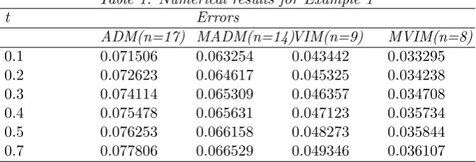
Table 1. Numerical results for Example 1
t Errors
ADM(n=17) MADM(n=14)VIM(n=9) MVIM(n=8)
0.1 0.071506 0.063254 0.043442 0.033295
0.2 0.072623 0.064617 0.045325 0.034238
0.3 0.074114 0.065309 0.046357 0.034708
0.4 0.075478 0.065631 0.047123 0.035734
0.5 0.076253 0.066158 0.048273 0.035844
0.7 0.077806 0.066529 0.049346 0.036107
t Errors
HPM(n=10) MHPM(n=8) HAM(n=5)
0.1 0.053415 0.034728 0.022347
0.2 0.054571 0.035502 0.022895
0.3 0.055018 0.036147 0.023203
0.4 0.055622 0.037639 0.024328
0.5 0.056236 0.038085 0.025185
Table 1, shows that, approximate solution of the Riccati equation is convergence with 5 iterations by using the HAM . By comparing the results of Table 1 , we can observe that the HAM is more rapid convergence than the ADM, MADM, VIM, MVIM, HPM and MHPM.
5
Conclusion
The HAM has been shown to solve effectively, easily and accurately a large class of nonlin-ear problems with the approximations which are convergent are rapidly to exact solutions. In this work, the HAM has been successfully employed to obtain the approximate solution to analytical solution of the comparing the results of Table 1 , we can observe that the HAM is more rapid convergence than the ADM, MADM, VIM, MVIM, HPM and MHPM..
Acknowledgments
The authors would like to express their sincere appreciation to the Department of Mathematics, Islamic Azad University, Central Tehran Branch for their cooperation.
References
[1] WT. Reid, Riccati differential equations (Mathematics in science and engineering), New York: Academic Press, 1972.
[2] BD. Anderson, JB. Moore, Optimal control-linear quadratic methods, Prentice-Hall, New Jersey, 1999.
[3] I. Lasiecka, R. Triggiani, Differential and algebraic Riccati equations with applica-tion to boundary/point control problems: continuous theory and approximaapplica-tion theory (Lecture notes in control and information sciences), Berlin: Springer, 1991.
[4] AA. Bahnasawi, MA. El-Tawil, A. Abdel-Naby, Solving Riccati differential equation using Adomians decomposition method, Appl. Math. Comput. 157 (2004) 503514.
[5] F. Dubois, A. Saidi, Unconditionally stable scheme for Riccati equation, ESAIM Pro-ceedings 8(2000) 3952.
[6] J. Biazar, M. Eslami,Differential Transform Method for Quadratic Riccati Differential Equation, International Journal of Nonlinear Science 9(2010)444-447.
[7] S. Abbasbandy, A new application of Hes variational iteration method for quadratic Riccati differential equation by using Adomians polynomials, J. Comput. Appl. Math. 207 (2007) 59-63.
[8] Y. Tan, S. Abbasbandy, Homotopy analysis method for quadratic Riccati differential equation, Commun. Nonlin. Sci. Numer. Simul. 13 (2008) 539-546.
[9] G. Mustafa, S. Mehmet,On the solution of the Riccati equation by the Taylor matrix method, Appl. Math. Comput. 176 (2006) 414-421.
[11] MA. Fariborzi Araghi, Sh . S. Behzadi, Solving nonlinear Volterra-Fredholm integral differential equations using the modified Adomian decomposition method, Comput. Methods in Appl. Math. 9 (2009) 1-11.
[12] AM. Wazwaz, Construction of solitary wave solution and rational solutions for the KdV equation by ADM, Chaos, Solution and fractals 12(2001) 2283-2293.
[13] AM. Wazwaz, A first course in integral equations, WSPC, New Jersey, 1997.
[14] IL. El-Kalla, Convergence of the Adomian method applied to a class of nonlinear integral equations, Appl. Math. Comput. 21 (2008) 372-376.
[15] JH. He, XH. Wu, Exp-function method for nonlinear wave equations, Chaos, Solitons and Fractals 30 (2006) 700-708.
[16] JH. He, Variational principle for some nonlinear partial differential equations with variable cofficients, Chaos, Solitons and Fractals 19 (2004) 847-851.
[17] JH. He, W.. Shu-Qiang, Variational iteration method for solving integro-differential equations, Physics Letters A 367 (2007) 188-191.
[18] JH. He, Variational iteration method some recent results and new interpretationsJ. Comp. Appl. Math. 207 (2007) 3-17.
[19] MA. Fariborzi Araghi, Sh. S. Behzadi, Numerical solution of nonlinear Volterra-Fredholm integro-differential equations using Homotopy analysis method, Journal of Applied Mathematics and Computing, DOI:10.1080/00207161003770394, 2010.
[20] TA. Abassy, E. Tawil, H. El. Zoheiry,Toward a modified variational iteration method, J. Comput. Apll. Math. 207 (2007) 137-147.
[21] TA. Abassy, E. Tawil, H. El. Zoheiry,Modified variational iteration method for Boussi-nesq equation, Appl. Math. Comput. 54 (2007) 955-965.
[22] SJ. Liao,Beyond Perturbation: Introduction to the Homotopy Analysis Method, Chap-man and Hall/CRC Press, Boca Raton, 2003.
[23] SJ. Liao, Notes on the homotopy analysis method: some definitions and theorems, Communication in Nonlinear Science and Numerical Simulation 14 (2009) 983-997.
[24] E. Babolian, J. Saeidian, Analytic approximate solutions to Burger, Fisher, Huxley equations and two combined forms of these equations, Commun Nonlinear Sci Numer Simulat. 14 (2009) 1984-1992.
[25] J. Biazar, H. Ghazvini, Convergence of the homotopy perturbation method for partial differential equations, Nonlinear Analysis: Real World Application 10 (2009) 2633-2640.
[27] A. Golbabai, B. Keramati, Solution of non-linear Fredholm integral equations of the first kind using modified homotopy perturbation method, Chaos Solitons and Fractals 5 (2009) 2316-2321.
[28] M. Javidi,Modified homotopy perturbation method for solving linear Fredholm integral equations, Chaos Solitons and Fractals 50 (2009) 159-165.
[29] MA. Fariborzi Araghi, S. Sh. Behzadi,Numerical solution for solving Burger’s-Fisher equation by using Iterative Methods, Mathematical and Computational Applications 16 (2011) 443-455.