Munich Personal RePEc Archive
Stock Return Predictability: Evaluation
based on Prediction Intervals
Charles, Amelie and Darne, Olivier and Kim, Jae
Audencia Nantes, University of Nantes, La Trobe University
18 March 2016
Online at
https://mpra.ub.uni-muenchen.de/70143/
Stock Return Predictability: Evaluation
based on Prediction Intervals
Am´
elie CHARLES
∗Audencia Nantes, School of Management
Olivier DARN´
E
†‡LEMNA, University of Nantes
Jae H. KIM
§Department of Economics and Finance, La Trobe University
∗Audencia Nantes, School of Management, 8 route de la Jonelire, 44312 Nantes, France. Email:
†LEMNA, University of Nantes, IEMN–IAE, Chemin de la Censive du Tertre, BP 52231, 44322
Nantes, France. Email: [email protected].
‡Olivier Darn´e gratefully acknowledge financial support from the Chaire Finance of the University of
Nantes Research Foundation.
§Corresponding Author: [email protected]; All computations are conducted using the VAR.etp
Abstract
This paper evaluates the predictability of monthly stock return using out-of-sample (multi-step ahead and dynamic) prediction intervals. Past studies have exclusively
used point forecasts, which are of limited value since they carry no information about the intrinsic predictive uncertainty associated. We compare empirical
per-formances of alternative prediction intervals for stock return generated from a naive model, univariate autoregressive model, and multivariate model (predictive
regres-sion and VAR), using the U.S. data from 1926. For evaluation free from data snooping bias, we adopt moving sub-sample windows of different lengths. It is found that the naive model often provides the most informative prediction
inter-vals, outperforming those generated from the univariate model and multivariate models incorporating a range of economic and financial predictors. This strongly
suggests that the U.S. stock market has been informationally efficient in the weak-form as well as in the semi-strong weak-form, subject to the inweak-formation set considered in this study.
Keywords: Autoregressive Model, Bootstrapping, Financial Ratios, Forecasting,
Interval Score, Market Efficiency
1
Introduction
Stock return predictability has been an issue of profound importance in empirical
finance. It has strong implications to investment decisions and strategies, as well as to the fundamental concepts such as market efficiency. The empirical literature is extensive, ranging from the seminal works of Campbell and Shiller (1988) and Fama
and French (1988) to the notable recent contributions such as Welch and Goyal (2008) and Neely et al. (2014). While a number of recent studies evaluate
out-of-sample predictability of stock return, they rely exclusively on point forecasting (e.g., Welch and Goyal, 2008; Campbell and Thompson, 2008; Lettau and Van
Nieuwerburgh, 2008; Rapach et al., 2010; Westerlund and Narayan, 2012). A point forecast is a single number as an estimate of the unknown future value. Although it may represent the most likely outcome from a predictive distribution,
it carries no information about the degree of intrinsic uncertainty or variability associated. For this reason, one may justifiably argue that comparison of point
forecasts only is of limited value for assessing predictability. As Chatfield (1993) and Christoffersen (1998) argue, interval forecast (or prediction interval) is of a higher value to decision-makers, allowing for a more complete and informative
evaluation of predictability (see also De Gooijer and Hyndman, 2006; Pan and Politis, 2016). This is particularly so for stock returns which show a high degree of
volatility over time. This paper contributes to the extant literature on stock return predictability by evaluating out-of-sample prediction intervals.
A prediction interval consists of an upper and a lower limit between which the future value is expected to lie with a prescribed probability (Chatfield, 1993). As an estimate of possible future scenario, it is substantially more informative
than a single value. It shows the possible direction of future value, also giving a clear indication about the extent of uncertainty associated. A tight interval
is informative to decision-makers, since they can be highly confident about the future outcome, given the prescribed probability content. In contrast, a wide one
carries little information about the future outcome, indicating a high degree of uncertainty. Prediction intervals can be generated from popular linear forecasting models available in many econometric packages, including the predictive regression
models for stock return (see, for example, Welch and Goyal, 2008; Amihud et. al, 2004; and Kim, 2014). Conventionally, a prediction interval is constructed
ignoring estimation uncertainty. An alternative is the bootstrap method, which provides a non-parametric approximation to the predictive distribution based on data resampling (see Pan and Politis, 2016). It is capable of generating prediction
intervals which take full account of estimation uncertainty and without resorting to the normality assumption.
In this paper, we consider prediction intervals based on a range of linear models, which are widely used in practice to predict stock return at the monthly frequency. For the univariate case, an autoregressive (AR) model is used. For the multivariate
case, the predictive regression and vector autoregressive (VAR) model are used. The AR model is constructed with an assumption that the stock return depends
on its own past only. The AR(0) model represents a naive model where the stock return has no dependency on its own past. The predictive regression specifies
that the stock return depends on the past of a predictor such as financial and macroeconomic variables (e.g., Welch and Goyal, 2008; Campbell and Thomson, 2008; Lettau and Van Nieuwerburgh, 2008; Rapach et al., 2010; Westerlund and
Narayan, 2012). The VAR model represents a general linear model which specifies the stock return as a function of its own past and the past of its predictor. For
the predictive regression and VAR models, we employ bias-corrected parameter estimation to construct prediction intervals free from small sample estimation bias
(see Stambaugh, 1999). We mainly consider prediction intervals generated based on the conventional normal approximation to the predictive distribution, but a bootstrap alternative is also considered. As a means of comparison, we use the
coverage rate and interval score (Gneiting and Raftery, 2007; p.370). While the former is a dichotomous measure as to whether prediction interval covers the true
value or not, the latter is a quality-based measure which captures both accuracy and variability of prediction.
To the best of our knowledge, this paper is the first study examining the stock
return predictability using prediction intervals. As already mentioned, the previ-ous studies exclusively evaluate point forecasts, often accompanied by predictive
ability tests. Our study represents the emphasis of estimation over testing, which more directly address the effect size of prediction. In light of the recent warnings
and concerns expressed by the American Statistical Association (Wasserstein and Lazar, 2016) for the scientific findings entirely based on the p-value approach to statistical significance, our study is unique and novel in the literature of stock
quality of prediction interval improves as additional information is incorporated into the model. If the AR(0) model is found to generate the prediction interval of the highest quality, this is an indication that the additional information such
as the past values of stock return or those of the predictors adds little value to the predictability of stock return. If a multivariate model with a particular
pre-dictor appears to be the clear winner, it serves as evidence that the prepre-dictor has a strong predictive power for stock return. We use the monthly data set compiled by Welch and Goyal (2008) for the U.S. stock market, which contains stock return
and a range of potential predictors from 1926 to 2014, including the dividend yield, dividend-payout ratio, book-to-market ratio, price-earnings ratio, inflation rate,
and risk-free rate. We extent these predictors by considering two macroeconomic variables (the industrial production growth and the output gap), because they are
found to be informative about expected business conditions (Cooper and Priestley, 2009; Schrimpf, 2010); and the index of economic policy uncertainty proposed by Baker et al. (2015) because the economic uncertainty is found to affect financial
markets (see, e.g., Bekaert et al., 2009; Brogaard and Detzel, 2015; Bali and Zhou, 2016). Evaluation of alternative out-of-sample prediction intervals is conducted in
a purely empirical setting by calculating the mean coverage rate and interval score using the realized future values. For evaluation free from data snooping bias and
possible structural changes, we apply moving sub-sample windows with a set of different window lengths.
The main finding of the paper is that the prediction intervals from the naive
AR(0) model often outperform those generated from the models with additional information content. The univariate and multivariate models show little evidence
of generating more accurate and informative prediction intervals than the AR(0) model. This suggests that the U.S. stock return has been unpredictable and that the market has been efficient in the weak and semi-strong forms, subject to the
information content considered on this study. The next section presents a brief review of the relevant literature. Section 3 presents the methodologies, and Section
4 presents the data and computational details with illustrative examples. The empirical results are discussed in Section 5, and the conclusion is drawn in Section
2
A Brief Literature Review
Given that the empirical literature of stock return predictability is broad and
ex-pansive, we provide a brief review of past studies focusing on those that evaluate out-of-sample predictability. We also point out the limitations of the past studies, and highlight the contribution of our study in the context of extant literature.
Whether stock return is predictable from an economic fundamental has been an issue of much interest and contention in empirical finance. The literature on return
predictability has brought more questions than answers. In the first models, such as Samuelson (1965, 1969) and Merton (1969), excess returns were assumed to be
unpredictable. However, the empirical literature in the 1980s has found variables with predictive power to explain stock returns (see, e.g., Keim and Stambaugh, 1986; Campbell and Shiller, 1988; Fama and French, 1988, 1989). After strong
evidence in favor of return predictability on the aggregate level in the 1990s and 2000s, recent empirical evidence considers that the predictability of stock return
is rather weak (see, e.g., Ang and Bekaert, 2007; Cochrane, 2008; Lettau and Van Nieuwerburgh, 2008; Welch and Goyal, 2008). More precisely, the evidence for U.S. stock return predictability seems to be predominantly in-sample, but it is not
robust to out-of-sample evaluations.1
The previous studies on stock return predictability evaluate the out-of-sample
(OOS) forecasting using various approaches (see Table 1). A number of stud-ies assess the OOS performance of the predictive regression models by comparing
the OOS R2 suggested by Campbell and Thompson (2008) and/or the root mean square errors (RMSE). Obviously, simply comparing RMSE does not take into ac-count the sample uncertainty underlying observed forecast differences. Therefore,
recent studies use predictive ability tests (Welch and Goyal, 2008; Rapach et al., 2010; Westerlund and Narayan, 2012). Westerlund and Narayan (2012) use the
equality predictive ability test proposed by Diebold and Mariano (1995) and the forecast encompassing test developed by Harvey et al. (1998) which compare OOS
forecasts from non-nested models. A drawback of these tests is that they have a nonstandard distribution when comparing forecasts from nested models (see Clark and McCracken, 2001; McCracken, 2007). In order to account for the nested
mod-1
els Welch and Goyal (2008) and Westerlund and Narayan (2012) apply the MSEF and ENCNEW statistics of McCracken (2004), and Clark and McCracken (2001), respectively. The McCracken (2004) test statistic is a variant of the Diebold and
Mariano (1995) statistic, while the Clark and McCracken (2001) test statistic is a variant of the Harvey et al. (1998) statistic. Rapach et al. (2010) use the
MSPE-adjusted statistic of Clark and West (2007) that is an MSPE-adjusted version of the Diebold-Mariano statistic allowing to compare forecasts from nested linear models. Methodologically, there are two limitations of the above-mentioned past studies
that examine out-of-sample predictability. First, as mentioned in the previous sec-tion, the analysis based on point forecasts only is of limited value since the
variabil-ity of prediction is not fully taken account (see Chatfield, 1993; and Christoffersen, 1998). Our paper contributes to the extant literature as the first study that adopts
the prediction interval as a means of assessing stock return predictability. Secondly, the recent statement made by the American Statistical Association (Wasserstein and Lazar, 2016) expresses a serious concern on the use ofp-value with an arbitrary
threshold of 0.05 in many scientific research. In particular, they warn that ”the widespread use of statistical significance (generally interpreted asp-value less than
0.05) as a license for making a claim of a scientific finding (or implied truth) leads to considerable distortion of the scientific process.” We note that the past studies
on return predictability (both in-sample and out-of-sample) rely heavily on the sta-tistical significance based onp-value in establishing their findings. Our study based on prediction interval represents an estimation-based investigation which directly
addresses the effect size of out-of-sample forecasting, which Wasserstein and Lazar (2016) suggest as a desirable alternative to statistical significance solely based on
thep-value criterion.
3
Methodology
In this section, we present the models for stock return prediction and the methods for generating out-of-sample prediction interval. These models have simple linear
structures and their specifications can be automatically determined by a fully data-dependent method without an intervention of a researcher. Throughout the paper, we use AIC (Akaike’s information criterion) to determine the unknown model
of size n (t = 1, ..., n), we generate a point forecast Yn(h) for the h-period ahead
future valueYn+hofY. Ah-step ahead prediction interval with probability content
100(1-2θ)% is denoted as P In(h, θ).
3.1
Univariate autoregression
We consider theAR(p) model of the form
Yt=α0+α1Yt−1+...+αpYt−p+ut (1)
whereutis an identically and independently (IID) distributed error term with zero
mean and fixed variance. The model specifies that the stock return is predictable
purely from its own past. An AR(0) model with αi = 0 for all i (i = 1, ..., p) is
used as a naive model where past returns have no predictive power for the future
return.
The unknown parameters are estimated using the least-squares (LS) method. The LS estimators for (α0, α1, ..., αp) are denoted as (αb0,αb1, ...,αbp) and the LS
residuals{but}nt=p+1. The point forecast forYn+h(h= 1,2, ..., H) is generated using
the LS estimators as
Yn(h) =αb0+bα1Yn(h−1) +...+αbpYn(h−p) (2)
whereYn(j) =Yn+j forj≤0. The 100(1-2θ)% prediction interval forYn+h can be
constructed based on the prediction mean-squared error (M SE(Yn(h))), obtained
using the delta method2 with the AR parameter estimators (αb0,αb1, ...,αbp) and
assuming the normality of prediction error distribution, as
P In(h, θ;AR)≡[Yn(h)−zτM SE(Yn(h)), Yn(h) +zτM SE(Yn(h))], (3)
where zτ is the 100(1−τ)% percentile of the standard normal distribution with
τ = 0.5θ.
3.2
Bootstrap prediction intervals
The prediction intervals given in the previous subsection are constructed based on
the assumption that the predictive error distribution follows a normal distribution.
2
The prediction MSE is calculated based on the delta method (Lutkepohl, 2005), which approximates the true variability based on asymptotic approximation. One may argue that the normality assumption is difficult to justify for stock return and
that the delta method may provide inaccurate estimation of the true variability of the predictive distribution. In addition, in constructing the prediction interval,
the conventional method does not account of estimation uncertainty. Hence, it is sensible to consider a non-parametric alternative which does not require the assumption of normality and asymptotic approximations.
The bootstrap is a method approximating the true sampling distribution of a statistic using the repetitive re-sampling the observed data, without imposing
normality or resorting to asymptotic approximation (Thombs and Schucany, 1990; Pan and Politis, 2106). For the univariate AR model, the bootstrap method can
be described as follows:
Generate the artificial set of data as
Y∗
t =αb0+bα1Yt∗+1+...+αbpYt∗+p+u∗t (4)
where (bα0, ...,bαp) are the LS estimators for (α0, ..., αp) andu∗t is random draw with
replacement from the LS residuals {ubt}nt=p+1. Note that we follow Thombs and
Schucany (1990) to generate {Y∗
t }nt=1 based on the backward AR model using the
lastpobservation as the starting values. This is to accommodate the conditionality of the AR parameter estimators on the lastp values of the series. Using {Y∗
t }nt=1,
the unknown AR parameters (α0, ..., αp) are re-estimated, which are denoted as
(αb∗
0, ...,αb∗p). The bootstrap replicates of the AR forecast for Yn+h, made at time
period n, are generated recursively as
Y∗
n(h) =αb∗0+αb∗1Yn∗(h−1) +...+bα∗pYn∗(h−p) +u∗n+h (5)
where Y∗
n(j) = Yn+j for j ≤ 0 and u∗t is random draw with replacement from
{ubt}nt=p+1.
Repeat (4) and (5) many times, say B, to yield the bootstrap distribution for
the AR forecast{Y∗
n(h;j)}Bj=1. This distribution is used as an approximation to the
predictive distribution for Yn+h. The 100(1-2θ)% prediction interval for Yn+h can
be constructed by taking appropriate percentiles from the bootstrap distribution.
That is,
P In(h, θ;AR∗)≡[Yn∗(h, τ), Yn∗(h,1−τ)], (6)
whereY∗
3.3
Predictive regression: IARM
We consider a predictive model for stock return Y as a function of a predictorX
with lag orderp, which can be written as
Yt=β0+β1Xt−1+...+βpXt−p+v1t (7)
Xt=δ0+δ1Xt−1+...+δpXt−p+v2t. (8)
It is assumed that the error terms are IID with fixed variances and covariances:
V ar(v1t)≡σ21, V ar(v2t)≡σ22 and Cov(v1t, v2t)≡σ12.
It is well-known that the LS estimators for (β1,..., βp) are biased in small samples, as long as σ12 ̸= 0. It is because the LS estimators completely ignore
the presence of σ12, as Stambaugh (1999) points out. Amihud et al. (2004, 2008,
2010) propose a bias-correction method based on a augmented regression, called the augmented regression method (ARM), which is subsequently improved by Kim
(2014).
The method assume that the error terms in (7) and (8) are linearly related as
v1t=ϕv2t+et whereetis an independent normal error term with a fixed variance.
It involves running the regression for Y against lagged X’s as in (7), augmented with the bias-corrected residuals from the predictor equations (8). That is, we run
the regression of the form
Yt=β0+β1Xt−1+...+βpXt−p+ϕvˆ
c
2t+et (9)
wherebvc
2t≡Xt−bδ c
0−bδ
c
1Xt−1−...−bδ
c
pXt−p, while (bδ
c
0,bδ
c
1, ...,bδ
c
p) are the bias-corrected
estimators for δi’s. Amihud et al. (2010) use the asymptotic formulae derived by
Shaman and Stine (1988) to obtain these corrected estimators. The
bias-corrected estimators (bβc0,βbc1, ...,bβcp) for (β0, β1, ..., βp) are obtained by regressing
the augmented regression (9).
Kim (2014) proposes three modifications to the ARM of Amihud et al. (2010).
The first is the bias-correction method of a higher order accuracy than the one used by Amihud et al. (2010). The second is the use of stationarity-correction
(Kilian, 1998), which ensures that the bias-corrected estimators satisfy the con-dition of stationarity. This correction is important because bias-correction often
easier. According to the Monte Carlo study of Kim (2014), the improved ARM (IARM) provides more accurate parameter estimation and statistical inference than its original version in small samples.
The point forecast for stock return based on the IARM is generated jointly with that of the predictor as
Yn(h) =βb c
0+bβ
c
1Xn(h−1) +...+bβ c
pXn(h−p) (10)
whereXn(h) =bδ c
0+bδ
c
1Xn(h−1)+...+bδ c
pXn(h−p) andXn(j) =Xn+jforj≤0. The
100(1-2θ)% prediction interval forYn+h can be constructed based on the prediction
mean-squared error (M SE(Yn(h))) obtained using the delta method with IARM
parameter estimators and assuming the normality of prediction error distribution.
That is,
P In(h, θ;IARM)≡[Yn(h)−zτM SE(Yn(h)), Yn(h) +zτM SE(Yn(h))]. (11)
3.4
Vector Autoregressive Model
The predictive model given (7) and (8) specifies that the stock return depends only
on the past value of a predictor. This means that the model allows for only one-way causality from the predictor to stock return, and that the stock return does
not depend on the past value of its own. These restrictions may deliver a simple and parsimonious model, but they completely exclude the possibility stock return depending on its own past and the potential feedback effect from stock return to
the predictor. A more general model can be specified by resorting to the vector autoregressive (VAR) model, which can be written as
Yt=τ0+α1Yt−1+...+αpYt−p+β1Xt−1+...+βpXt−p+u1t (12) Xt=τ0+γ1Yt−1+...+γpYt−p+δ1Xt−1+...+δpXt−p+u2t. (13)
The model is widely used for modeling and forecasting stock return dynamically
inter-related with other predictors (see, for example, Engsted and Pedersen, 2012). The LS estimator for the unknown parameters in (12) and (13) are biased in
Killian’s (1998) stationarity correction in case the bias-correction provides param-eter estimates which imply non-stationarity. Using these bias-corrected estimators, the point forecasts are generated recursively as
Yn(h) =eτ0+eα1Yn(h−1) +...+αepYn(h−p) +βe1Xn(h−1) +...+eβpXn(h−p)(14)
Xn(h) =eτ0+eγ1Yn(h−1) +...+γepYn(h−p) +eδ1Xn(h−1) +...+eδpXn(h−p).(15)
where Xn(j) =Xn+j for j ≤0,Yn(j) = Yn+j forj ≤0, and the parameters with
tilde indicates the bias-corrected estimator for the corresponding parameters.
The 100(1-2θ)% prediction interval for Yn+h, constructed based on the
predic-tion mean-squared error (M SE(Yn(h))) obtained using the delta method with the
VAR bias-corrected parameter estimators and assuming the normality of prediction error distribution, is denoted as
P In(h, θ;V AR)≡[Yn(h)−zτM SE(Yn(h)), Yn(h) +zτM SE(Yn(h))]. (16)
4
Data and Computational Details
In this section, we provide the data and computational details, along with the simple illustrative examples in relation to interval forecasting and their assessment.
4.1
Data
We use the financial variables compiled by Welch and Goyal (2008) for the U.S.
stock market, available from Amit Goyal’s website. The precise definitions of these variables are given in Welch and Goyal (2007). For stock return, we use the CRSP
NYSE value-weighted return, which is widely used as a benchmark for investment and academic research. These financial variables (monthly from 1926 to 2014, except for NTIS which starts from 1927) are listed as below:
• Dividend-Yield (DY)
• Dividend-Price Ratio (DP)
• Earnings-Price Ratio (EP)
• Dividend Payout Ratio (DE)
• Risk-free rate (RF)
• Inflation (INF)
• Stock Variance (SVAR)
• Long Term Yield (LTY)
• Long Term Return (LTR)
• Net Equity Expansion (NTIS)
• Default Return Spread (DFR)
• Default Yield Spread (DFY)
• Term Spread (TMS)
We add three economic variables (monthly from 1927 to 2014) to those proposed by Welch and Goyal (2008):
• Industrial production growth (IPG)
• Output gap (GAP)
• Economic policy uncertainty (EPU)
The data used to construct the industrial production growth and the output
gap are downloaded from the FRED database of St Louis Fed. Following Schrimpf (2010) we construct the output gap measure by applying the filter by Hodrick and
Prescott (1997) to the logarithmic series of industrial production. The smoothing parameter is set to 128,800 (monthly data). The cyclical component of the series
is taken as the output gap. The index of economic policy uncertainty (EPU) is proposed by Baker et al. (2015), built on three components: (i) the frequency of newspaper references to economic policy uncertainty, (ii) the number of federal tax
code provisions set to expire, and (iii) the extent of forecaster disagreement over future inflation and government purchases.3
4.2
Computational Details
Evaluation of alternative out-of-sample prediction intervals is conducted in a purely
empirical setting using the realized future values. For evaluation free from data
3
snooping bias, we apply moving sub-sample windows to the above data set, adopt-ing a grid of different estimation window lengths rangadopt-ing from 24 months to 240 months (with an increment of 24 months). From each estimation window, 12-step
ahead (out-of-sample) prediction intervals are generated from a predictive model. For example, when the window length of 24 months, we take the first 120
ob-servations from January 1926 to estimate the model, and generate 12-step ahead forecasts. And then we move to the next set of 120 observations from February 1926 to estimate the model and generate forecasts. This continues until the end of
the data set is reached.
As a means of comparison, we use the coverage rate and the interval score
proposed by Gneiting and Raftery (2007, p.370). Let a 100(1−2θ)%h-step ahead prediction interval be given by [Lh, Uh]. The coverage rate is calculated as the
proportion of the true values covered by the prediction interval, i.e.,
C(h) = ♯(Lh ≤Yh≤Uh)
N ,
whereYh is the true future value,N is the total number of prediction intervals for
forecast horizon h, and ♯indicates the frequency at which the condition inside the bracket is satisfied. A 100(1−2θ)% prediction interval is expected to have C(h) value of (1−2θ) in repeated sampling.
The interval score for a 100(1−2θ)% interval [Lh, Uh], it is given by
Sθ(Lh, Uh;Yh) = (Uh−Lh) +
1
θ(Lh−Yh)I(Yh< Lh) +
1
θ(Yh−Uh)I(Yh> Uh)
whereI(·) is an indicator function which takes 1 if the condition inside the bracket is satisfied and 0 if otherwise; andYh is the true future value. If the interval covers
Yh, the score takes the value of its length; if otherwise, a penalty term is added
to the value of length, which is how much the interval misses Yh scaled by 1/θ.
In the event that the interval misses Yh by a small (large) margin, a light (heavy)
penalty is imposed. The interval score measures the quality of the probabilistic
statement implied by a prediction interval. We note that the interval score is far more informative than the coverage rate, since it takes full account of the accuracy and riskiness of a prediction interval. In fact, the dichotomous nature of
the coverage rate may deliver misleading assessment of predictive accuracy, as the examples in the next subsection show. Hence, in this paper, we use both measures,
4.3
Examples
In this subsection, we present three simple illustrative examples. The first high-lights the reason as to why evaluation of point forecasts only is an incomplete exercise in assessing predictability; while the other two explain why the interval
scoreSθ is a more informative measure of predictive quality than the coverage rate
C(h) presented in Section 4.2.
Consider a set of future values (y1, y2, y3, y4, y5) = (0,0,0,0,0), along with two
sets of 80% prediction intervalsP I1andP I2generated from two alternative models
(called Model 1 and Model 2):
Example 1: Point Forecasting versus Interval Forecasting
P I1= [(−1,1),(−1,1),(1,2),(−1,1),(−1,1)]
P I2= [(−2,2),(−2,2),(0.5,2.5),(−2,2),(−2,2)]
For the purpose of simplicity, suppose that Models 1 and 2 generate the identical point forecasts, which means that the two appear to show the predictive accuracy of
the same degree if evaluation is carried out using the point forecasts only. However, Model 2 generates prediction intervals twice wider than Model 1, indicating that its prediction is twice riskier than that of Model 1. In this case, Model 1 should be
clearly preferred for the purpose of forecasting. If Model 2 includes an information set additional to that of Model 1, the extra information does not improve the
quality of prediction but only increases its variability. An important point is that comparison based on point forecasts is not capable of capturing the difference in
forecast variability.
Example 2: Coverage Rate versus Interval Score
P I1= [(−1,1),(−1,1),(1,2),(−1,1),(−1,1)]
P I2 = [(0.1,0.2),(−0.2,−0.1),(0.1,0.2),(−0.2,−0.1),(0.1,0.2)]
P I1 covers the true values (y) four out of five times, with the correct coverage
rate of 0.8; while P I2 never covers the true value and its coverage rate is 0. If one
adopts the coverage rate as a means of comparison, the Model 1 should be preferred. However, the mean interval score ofP I1 is 3.8 and that ofP I2 is 1.1, which means
becauseP I2’s are much tighter, only narrowly missing the true values. In contrast,
P I1’s are too wide and uninformative. In this case, the coverage rate fails to capture
the richer informative quality of P I2.
Example 3: Coverage Rate versus Interval Score
P I1 = [(−0.5,0.5),(−0.5,0.5),(1.5,2.5),(−0.5,0.5),(−0.5,0.5)]
P I2 = [(−0.5,0.5),(−0.5,0.5),(0.1,1.1),(−0.5,0.5),(−0.5,0.5)]
P I1 and P I2 have the correct coverage rate of 0.8 and identical lengths. However,
the mean interval score of P I1 is 4 while that of P I2 is 1.2. This is because P I1
misses by big margin when it fails to cover the true value, while P I2 misses it
only with a small margin. As before, the coverage rate does not fully reflect the
informative quality of prediction interval because it is unable to capture the effect of a big miss (which can be costly economically), while the interval score is capable of including this costly miss in its evaluation.
5
Empirical Results
Given the large number of possible predictors for stock return and the prediction
models being considered, we report only a set of selective but representative re-sults. This is to simplify the exposition and to present the results in a manageable
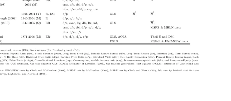
way. However, we note that qualitatively similar results are obtained from those unreported. Figure 1 plots the examples of 50% and 95% prediction intervals for
stock return, 1-step ahead from 1936:01 to 2014:12 generated with rolling window of length 120. The first figure plots those from the AR(0) model and the second those from the IARM with the dividend yield (DY) as a predictor. As might be
expected, 95% intervals are wider but less informative, while 50% intervals are tighter but riskier with a higher chance of missing the true values. The width of
the intervals changes over time, wider during the periods of higher volatility. The main question of the paper is whether additional information included in the pre-dictive model can improve the informative quality of prediction intervals for stock
return.
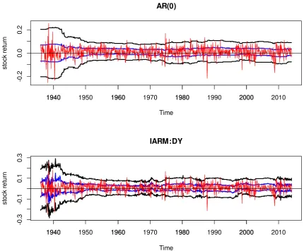
We first check whether the prediction intervals provide reasonable coverage
of prediction interval proposed by Christoffersen (1998). It is based on the property that, for 100(1-2θ)% prediction intervals to be efficient (conditionally on the past information), the indicator variable for their coverage should follow the independent
Bernoulli distribution with parameter 1-2θ. Christoffersen (1998) develops the LR test for the joint null hypothesis for the coverage rate (1-2θ) and independence,
which asymptotically follows the chi-squared distribution with 2 degrees of freedom. Figure 2 plots the LR statistics for the prediction intervals from AR(0) model given in Figure 1, using the rolling sub-sample window of 120 observations. For the 50%
intervals, the joint hypothesis is rejected at 1% level of significance only occasionally over time; while for the 95% intervals, the hypothesis cannot be rejected at the
1% level over the entire period. Testing at the 5% level provides similar results. This indicates that the prediction intervals generated from the AR(0) model show
reasonable coverage properties over time. We note that those generated from the other models (such as the IARM with the predictor DY) provide similar results.
We now pay attention to the interval score properties of alternative prediction
intervals. As we have seen in the previous section, the interval score is a more com-plete measure for the quality of prediction interval than the coverage rate. Figure
3 reports the mean interval score of all prediction intervals for forecast horizon h
from 1 to 12. The multivariate models (IARM and VAR) have the predictor DY.
When the window length is 24, the mean score of the AR(0) and AR(p) models are the smallest for all forecast horizons, for both cases of 50% and 95% prediction intervals. When the window length is 120, again the univariate prediction intervals
show better performance than the multivariate ones in most cases. Hence, there is no clear evidence that inclusion of DY improves the predictability of stock
re-turn. In fact, the VAR model (which has the most general dependency structure) provides prediction intervals with the lowest quality in terms of the interval score. Figure 4 reports the mean interval score averaged across all forecast horizon
(median) for all prediction intervals. These median of mean interval scores are plotted against the window length from 24 to 240. As before, the multivariate
models have the DY as a predictor. Again, the prediction intervals generated from the univariate models outperform those from the multivariate models for nearly all
window lengths. Hence, the evidence suggests that the use of DY as a predictor does not improve predictability of stock return. It can also be observed that the accuracy improves with the sample size only to a certain point. For example, when
sam-ple size (or window length) is around 100, for both cases of 50% and 95% prediction intervals. In addition, as is also clear from Figure 3, we find no evidence that the bootstrap prediction intervals perform better than those generated from AR(0) or
AR(p) models. This suggests that the prediction intervals based on the conven-tional normal approximation to the predictive distribution perform adequately for
monthly stock return.
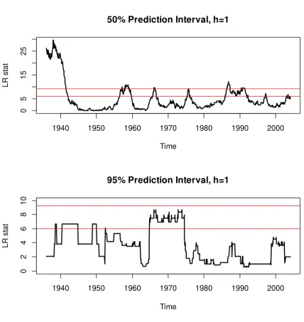
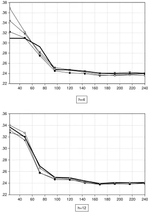
In Figure 5, the mean interval scores of the AR(0) model are compared with those from the IARM with different predictors including DY, DP, EP, BM, PE,
inflation rate, and risk-free rate, for forecast horizons 1, 4, 8, and 12. For h = 1, the AR(0) model shows smaller mean interval scores than the IARM for most
cases, especially when the length of rolling window is short. When forecast horizon is long (h = 8 or 12), there are occasions where the prediction intervals from IARM
beat those from the AR(0), but the margins are fairly small. When the rolling window length is greater than 120, the performances of the alternative prediction intervals are almost indistinguishable. That is, there is no compelling evidence that
the IARM with a range of predictors beats AR(0) model in terms of the interval score.
Figure 6 plots the mean interval scores from the economic variables (IPG, GAP, and EPU) based on the IARM for the forecast horizons 1, 4, 8, and 12, in
compar-ison with the score from the AR(0) model. Again, there is little evidence that the economic indicators help generate prediction intervals that are of higher quality than those from the AR(0) model. There are occasions where the mean
inter-val score from an economic variable is lower than that of AR(0) model, but the marginal improvement is fairly small. As also observed in Figure 5, when h = 1
and the window length is short, the AR(0) model is the clear winner. This means that, for short-term and short-horizon prediction of stock return, the naive AR(0) model provides the prediction intervals of the highest quality.
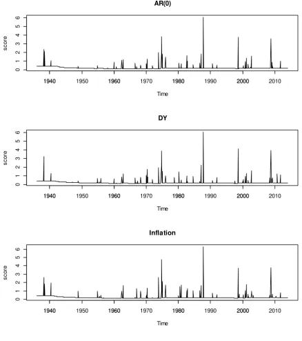
Figure 7 plots time variation of interval score when the window length is 120 and h = 1, for the AR(0) model and IARM with selected predictors. The spikes
represent the failure of prediction interval in predicting the future stock return. It appears that all prediction intervals show similar pattern over time, showing
the spikes at the times of stock market volatility, such as late 30’s, early 60’s, oil shock, and stock market crashes (1987, 2008). There is no clear evidence that any predictors from the IARM generate more accurate than AR(0) model. In
of predictive failure are not related with the business cycle.
The empirical results shown that there is no clear indication that the multivari-ate model with predictors beats the most simple and naive AR(0) model, in terms
of predictive accuracy and informative quality of prediction intervals. This finding points to the conclusion that the stock return has been unpredictable in the U.S.
market and that the stock market has been informationally efficient in the weak and semi-strong form, subject to the information set under investigation in this study.
6
Concluding Remarks
This paper contributes to the extant literature of stock return predictability, as the first study that adopts prediction interval as a measure of out-of-sample pre-dictability. Past studies exclusively used point forecasts, which are of limited value
in assessing predictability of stock return which often shows a high degree of volatil-ity over time. A point forecast is an estimate of the mean of the predictive
distribu-tion, which carries no information about its variability. A more complete analysis of predictive distribution can be achieved by evaluating prediction intervals (see Chatfield, 1993; Christoffersen, 1998, and Pan and Politis, 2015). We consider
pre-diction intervals for monthly stock return generated from a range of linear models with different degrees of information content. They include a naive model,
sim-ple linear univariate autoregressive models, and multivariate (predictive regression and vector autoregressive model). For the latter, we use a range of economic and
financial variables as possible predictors for stock return. We also consider the bootstrap prediction interval which relies on a non-parametric method and does not require the assumption of normality. In view of the recent statement made
by the American Statistical Association which expresses serious concerns on the research practice heavily based on statistical significance (Wasserstein and Lazar,
2016), our study represents an attempt to address the issue of stock return pre-dictability based on an estimation-based approach. In contrast, the past studies
rely heavily on statistical significance using thep-value as an indicator.
Using the data set compiled by Welch and Goyal (2007) with three additional economic variables, we evaluate and compare out-of-sample and multi-step
moving-subsample windows of different lengths. The mean coverage rate and interval score are used as the measures for predictive accuracy and quality of prediction intervals. We find that all models considered provide prediction intervals with reasonable
coverage properties. In terms of the interval score, we find that the AR(0) model, which is the most naive model, provides the prediction intervals that often
out-perform those generated from its univariate and multivariate alternatives. We find no clear indication that univariate autoregression and multivariate models provide prediction intervals of higher quality than those from the AR(0). That is, we find
little evidence that predictability of stock return is improved by incorporating the past history of its own and that of its predictors. The evidence suggests that the
U.S. stock market has been efficient in the weak-form as well as in the semi-strong form, subject to the information set considered in this study.
There are two further issues that future studies may explore. First, the pre-dictors not considered in this study may be examined. The universe of possible predictors for stock return is expansive, and we are calling for additional future
studies to evaluate their predictive power in the context of interval forecasting. For example, recent studies (based on point forecasting) report that technical
indica-tors show a higher degree of predictability than financial ratios (see, for example, Neely et al., 2014). Since we are limited by data availability for technical indicators
due to the historical span of the dataset in this study, future studies may assess the predictive power of technical indicators for interval forecasting of stock return. Second, only the prediction intervals generated from linear time series models are
considered in this study. It is possible that stock returns show non-linear depen-dence on past information (see Hinich and Patterson, 1985), while this possibility
has not been extensively investigated in the empirical literature of stock return predictability. In addition to the difficulty of finding a suitable non-linear model for stock return, we note that construction of prediction interval from a non-linear
model is a technically and computationally challenging exercise (see, for example, Frances and van Dijk, 2000). On this basis, this line of research is left as a possible
References
[1] Amihud, Y., Hurvich, C.M., 2004. Predictive regression: A reduced-bias
esti-mation method. Journal of Financial and Quantitative Analysis, 39, 813841.
[2] Amihud, Y., Hurvich, C.M., Wang, Y., 2008. Multiple-predictor regressions:
Hypothesis testing. Review of Financial Studies, 22, 413434.
[3] Amihud, Y., Hurvich, C.M., Wang, Y., 2010. Predictive regression with order-p autoregressive order-predictors. Journal of Emorder-pirical Finance, 17, 513525.
[4] Ang, A., Bekaert, G., 2007. Stock return predictability: Is it there? Review
of Financial Studies, 20, 651-707.
[5] Baker, S.R., Bloom, N., and Davis S.J., 2015. Measuring Economic Policy
Uncertainty, Working paper No 21633, NBER.
[6] Bali, T.G., Zhou, H., 2016. Risk, uncertainty, and expected returns. Journal of Financial and Quantitative Analysis, forthcoming.
[7] Bekaert, G., Engstrom, E., Xing, Y., 2009. Risk, uncertainty, and asset prices. Journal of Financial Economics, 91, 59-82.
[8] Brogaard, J., Detzel, A., 2015. The asset pricing implications of government
economic policy uncertainty. Management Science, 61, 3-18.
[9] Campbell, J.Y., Shiller, R.J., 1988. Stock prices, earnings, and expected divi-dends. Journal of Finance, 43, 661-76.
[10] Campbell, J.Y., Thompson, S.B., 2008. Predicting the equity return premium out of sample: Can anything beat the historical average? The Review of
Financial Studies, 21, 1509-1531.
[11] Chatfield, C., 1993. Calculating interval forecasts. Journal of Business and Economic Statistics, 11(2), 121-135.
[12] Christoffersen, P.F., 1998. Evaluating interval forecasts. International Eco-nomic Review, 39, 841-862.
[13] Clark, T., West, K., 2007. Approximately normal tests for equal predictive
accuracy in nested models. Journal of Econometrics, 138, 291-311.
[15] Cooper, I., Priestley, R., 2009. Time-varying risk premia and the output gap. Review of Financial Studies, 22, 2801-2833.
[16] Dangl, T., Halling, M., 2012. Predictive regressions with time-varying
coeffi-cients. Journal of Financial Economics, 106, 157-181.
[17] De Gooijer, J., Hyndman, R.J., 2006. 25 years of time series forecasting. In-ternational Journal of Forecasting, 22, 443473.
[18] Diebold, F., Mariano, R., 1995. Comparing predictive accuracy. Journal of
Business and Economic Statistics, 13, 253-263.
[19] Engsted, T., Pedersen, T.Q., 2012. Return predictability and intertemporal asset allocation: Evidence from a bias-adjusted VAR model. Journal of
Em-pirical Finance, 19, 241-253.
[20] Fama, E. F., K. R. French., 1988. Dividend yields and expected stock returns.
Journal of Financial Economics, 2(1), 3-25.
[21] Fama, E. F., K. R. French., 1989. Business conditions and expected returns on stocks and bonds. Journal of Financial Economics, 25(1), 23-49.
[22] Frances, P.H. van Dijk, D., 2000. Non-Linear Time Series Models in Empirical
Finance, Cambridge University Press, Cambridge.
[23] Gneiting, T., Raftery, A.E., 2007. Strictly proper scoring rules, prediction, and estimation. Jourmal of American Statistical Association, 102, 359378.
[24] Harvey D.I., Leybourne S.J., Newbold P., 1998. Tests for forecast encompass-ing. Journal of Business and Economic Statistics, 16, 254-259.
[25] Hinich, M.J., Patterson, D.M., 1985. Evidence of nonlinearity in daily stock
returns. Journal of Business and Economic Statistics, 3, 69-77.
[26] Hodrick, R.J., Prescott, E., 1997. Postwar U.S. business cycles: An empirical investigation. Journal of Money, Credit and Banking, 29, 1-16.
[27] Keim, D.B., Stambaugh R.F., 1986. Predicting returns in the stock and bond markets. Journal of Financial Economics, 17(2), 357-90.
[28] Kim, J.H., 2014. Predictive regression: An improved augmented regression
method. Journal of Empirical Finance, 26, 13-25.
[29] Kim. J.H., 2015. VAR.etp: VAR modelling: estimation, test-ing, and prediction. R package version 0.61. URL:
[30] Kilian, L. 1998. Small-sample confidence intervals for impulse response func-tions. The Review of Economics and Statistics, 80(2), 218-230.
[31] Kilian, L. 1999. Exchange rates and monetary fundamentals: What do we learn from long-horizon regressions? Journal of Applied Econometrics, 14,
491-510.
[32] Lettau, M., Van Nieuwerburgh, S., 2008. Reconciling the return predictability evidence. The Review of Financial Studies, 21(4), 1607-1652.
[33] Lewellen, J., 2004. Predicting returns with financial ratios. Journal of Financial Economics, 74, 209-235.
[34] L utkepohl, H., 2005. New Introduction to Multiple Time Series Analysis.
Springer.
[35] Mark, N.C., 1995. Exchange rates and fundamentals: Evidence on long-horizon predictability. American Economic Review, 85, 201-218.
[36] Merton, R.C., 1969. Lifetime portfolio selection under uncertainty: The continuous-time case. The Review of Economics and Statistics, 51 (3), 247-57.
[37] Neely, C.J., Rapach, D.E., Tu, J., Zhou, G., 2014. Forecasting the equity risk
premium: The role of technical indicators. Management Science, 60, 1772-1791.
[38] Nelson, C., Kim, M., 1993. Predictable stock return: The roles of small sample bias. The Journal of Finance, 48, 641-661.
[39] Nicholls, D.F., Pope, A.L., 1988. Bias in the estimation of multivariate
au-toregressions. Australian & New Zealand Journal of Statistics, 30A, 296-309.
[40] Pan, L., Politis, D.N., 2016. Bootstrap prediction intervals for linear, nonlin-ear and nonparametric autoregressions. Journal of Statistical Planning and Inference, forthcoming. Available online 7 November 2014, ISSN 0378-3758,
http://dx.doi.org/10.1016/j.jspi.2014.10.003.
[41] Pastor, L., Stambaugh, R.F., 2001. The equity premium and structural breaks. The Journal of Finance, 56, 1207-1239.
[43] Rapach, D.E., Strauss, J.K., Zhou, G., 2010. Out-of-sample equity premium prediction: Combination forecasts and links to the real economy. The Review of Financial Studies, 23, 821-862.
[44] Rapach, D.E., Strauss, J.K., Zhou, G., 2013. International stock return
pre-dictability: What is the role of the United States? The Journal of Finance, 68, 1633-1662.
[45] R Core Team, 2015. R: A language and environment for statistical com-puting. R Foundation for Statistical Computing, Vienna, Austria. URL
http://www.R-project.org/.
[46] Samuelson, P.A., 1965. Proof that properly anticipated price fluctuate ran-domly. Industrial Management Review, 6(2), 41-43.
[47] Samuelson, P.A., 1969. Lifetime portfolio selection by dynamic stochastic pro-gramming. The Review of Economics and Statistics, 51(3), 239-46.
[48] Schrimpf, A., 2010. International stock return predictability under model
un-certainty. Journal of International Money and Finance, 29, 1256-1282.
[49] Stambaugh, R.F., 1999. Predictive regressions. Journal of Financial Eco-nomics, 54, 375-421.
[50] Thombs, L.A., Schucany, W.R., 1990. Bootstrap prediction intervals for au-toregression. Journal of the American Statistical Association, 85, 486-492
[51] Wasserstein R. L. Lazar, N. A. 2016, The ASA’s statement on
p-values: Context, process, and purpose, The American Statistician, DOI: 10.1080/00031305.2016.1154108
[52] Welch, I., Goyal, A., 2008. A Comprehensive look at the empirical performance of equity premium prediction. The Review of Financial Studies, 21(4),
1455-1508.
[53] Westerlund, J., Narayan, P.K., 2012. Does the choice of estimator matter when forecasting returns? Journal of Banking and Finance, 36, 2632-2640.
[54] Westerlund, J., Narayan, P.K., 2015. Testing for predictability in conditionally
Table 1: Selected studies on the US stock return predictability.
Studies Sample Dep. Indep. Methodologies
Variables Variables Estimator In-sample Out-of-sample Welch and Goyal (2007) 1926-2005 (M) ER d/e, svar, lty, dfr, ltr, inf, OLS with R2 R2, ∆RMSE
tms, dfy, tbl, d/p, e/p, d/y, bootstrapped MSE-F & ENC-NEW tests ntis, eqis, b/m, e10/p, csp, cay F-stat
Campbell and sample start ER d/e, lty, inf, OLS R2 R2
Thompson (2008) 2005 (M) tms, dfy, tbl, d/p, e/p, ntis, b/m, e10/p, cay, roe
Lettau and 1926-2004 (Y) R, DG d/p OLS R2 R2
Van Nieuwerburgh (2008) 1946-2004 (M) R d/p, e/p, b/m
Rapach et al. (2010) 1947-2005 (Q) ER d/e, svar, lty, dfr, ltr, inf, OLS R2,
tms, dfy, tbl, d/p, e/p, d/y, MSPE & MHLN tests ntis, b/m, i/r
Westerlund and 1871-2008 (M) ER d/e, d/p, d/y, e/p OLS, AOLS, Theil U and DM,
Narayan (2012) FGLS MSE-F & ENC-NEW tests
Dependent variables: Excess stock returns (ER), Stock returns (R), Dividend growth (DG).
Independent variables: Dividend Payout Ratio (d/e), Stock Variance (svar), Long Term Yield (lty), Default Return Spread (dfr), Long Term Return (ltr), Inflation (inf), Term Spread (tms), Default Yield Spread (dfy), T-Bill Rate (tbl), Dividend Price Ratio (d/p), Earning Price Ratio (e/p), Dividend Yield (d/y), Net Equity Expansion (ntis), Percent Equity Issuing (eqis), Book to Market (b/m), Earning(10Y) Price Ratio (e10/p), Cross-Sectional Premium (csp), Consumption, wealth, income ratio (cay), Investment-to-capital ratio (i/k), real Return-on-Equity (roe). Methodologies: Estimators: the OLS estimator, the bias-adjusted OLS (AOLS) estimator of Lewellen (2004), the feasible generalized least squares (FGLSs) estimator of Westerlund and Narayan (2015).
Out-of-sample (OOS) tests: ENC-NEW tests by Clark and McCracken (2001), MSE-F test by McCracken (2007), MSPE test by Clark and West (2007), DM test by Diebold and Mariano (1995), MHLN test by Harvey, Leybourne, and Newbold (1998).
2
Figure 1. Examples of Prediction Intervals (50% and 95%, h=1, rolling window size =120)
The black lines represent 95% prediction intervals, the blue lines 50% intervals, and the red line indicates the stock return.
AR(0)
Time
st
o
c
k r
e
tu
rn
1940 1960 1980 2000
-0
.2
0
.0
0
.2
1940 1950 1960 1970 1980 1990 2000 2010
IARM:DY
Time
st
ock r
e
tu
rn
1940 1960 1980 2000
-0
.3
-0
.1
0
.1
0
.3
Figure 2. Likelihood Ratio Test Statistic for Prediction Intervals from AR(0) model (rolling
window size =120)
The red horizontal lines correspond to 5.99 and 9.21, which are 5% and 1% critical values from the chi-squared distribution with two degrees of freedom.
50% Prediction Interval, h=1
Time
LR
s
tat
1940 1950 1960 1970 1980 1990 2000
0
5
15
25
95% Prediction Interval, h=1
Time
LR
st
a
t
1940 1950 1960 1970 1980 1990 2000
02
4
68
1
.24 .28 .32 .36 .40 .44 .48 .52 .56
1 2 3 4 5 6 7 8 9 10 11 12
.125 .130 .135 .140 .145 .150 .155 .160 .165
1 2 3 4 5 6 7 8 9 10 11 12
.240 .244 .248 .252 .256 .260
1 2 3 4 5 6 7 8 9 10 11 12
.110 .112 .114 .116 .118 .120 .122
[image:29.842.112.728.84.514.2]1 2 3 4 5 6 7 8 9 10 11 12
Figure 3. Mean Score of Prediction Intervals
window length=24, 95% window length=24, 50%
.22 .24 .26 .28 .30 .32 .34 .36 .38
0 20 40 60 80 100 120 140 160 180 200 220 240
.10 .11 .12 .13 .14 .15
0 20 40 60 80 100 120 140 160 180 200 220 240
Open Circle: AR(0), Dark Circle: AR(p), Dark Square: AR(p) Bootstrap; Open Square: IARM; Cross: VAR
The predictor used in the IARM and VAR is DY (dividend-yiled).
[image:30.842.53.781.171.409.2]The mean score values plotted are median value over the forecast horizon 1, ...,12.
.20 .24 .28 .32 .36 .40
40 60 80 100 120 140 160 180 200 220 240
.20 .24 .28 .32 .36 .40 .44
40 60 80 100 120 140 160 180 200 220 240
.20 .24 .28 .32 .36 .40
40 60 80 100 120 140 160 180 200 220 240
.22 .24 .26 .28 .30 .32 .34 .36
40 60 80 100 120 140 160 180 200 220 240
h=4
Solid Line: AR(0); dark circile: BM; open circle: DP; cross: DY;
[image:31.842.462.757.78.502.2]h=12
Figure 5. Mean Interval Score of Alternative 95% Prediction Intervals (Financial Predictors)
h=1
.20 .24 .28 .32 .36 .40
40 60 80 100 120 140 160 180 200 220 240
.22 .24 .26 .28 .30 .32 .34 .36 .38
40 60 80 100 120 140 160 180 200 220 240
.22 .24 .26 .28 .30 .32 .34
40 60 80 100 120 140 160 180 200 220 240
.22 .24 .26 .28 .30 .32 .34 .36
[image:32.842.460.765.82.519.2]40 60 80 100 120 140 160 180 200 220 240
Figure 6. Mean Interval Score of Alternative 95% Prediction Intervals (Economic Predictors)
h=1 h=4
Figure 7. Plot of Interval Scores over time (h=1, rolling window length =120)
AR(0)
Time
sco
re
1940 1960 1980 2000
0
1234
56
1940 1950 1960 1970 1980 1990 2000 2010
DY
Time
sco
re
1940 1960 1980 2000
0123
456
1940 1950 1960 1970 1980 1990 2000 2010
Inflation
Time
sco
re
1940 1960 1980 2000
01
23
4
5
6
Note: The IARM is used for the model with predictors
SVAR
Time
sco
re
1940 1960 1980 2000
0
5
10
15
1940 1950 1960 1970 1980 1990 2000 2010
EPU
Time
sco
re
1940 1960 1980 2000
0
1234
5