Looking at word meaning An interactive visualization of Semantic Vector Spaces for Dutch synsets

Looking at word meaning.

An interactive visualization of Semantic Vector Spaces for Dutch synsets

Kris Heylen, Dirk Speelman and Dirk Geeraerts

QLVL, University of Leuven

Blijde-Inkomsstraat 21/3308, 3000 Leuven (Belgium)

{kris.heylen, dirk.speelman, dirk.geeraerts}@arts.kuleuven.be

Abstract

In statistical NLP, Semantic Vector Spaces (SVS) are the standard technique for the automatic modeling of lexical semantics. However, it is largely unclear how these black-box techniques exactly capture word meaning. To explore the way an SVS struc-tures the individual occurrences of words, we use a non-parametric MDS solution of a token-by-token similarity matrix. The MDS solution is visualized in an interac-tive plot with the Google Chart Tools. As a case study, we look at the occurrences of 476 Dutch nouns grouped in 214 synsets.

1 Introduction

In the last twenty years, distributional models of semantics have become the standard way of mod-eling lexical semantics in statistical NLP. These models, aka Semantic Vector Spaces (SVSs) or Word Spaces, capture word meaning in terms of frequency distributions of words over co-occurring context words in a large corpus. The basic assumption of the approach is that words occurring in similar contexts will have a simi-lar meaning. Speficic implementations of this general idea have been developed for a wide va-riety of computational linguistic tasks, includ-ing Thesaurus extraction and Word Sense Dis-ambiguation, Question answering and the model-ing of human behavior in psycholmodel-inguistic experi-ments (see Turney and Pantel (2010) for a general overview of applications and speficic models). In recent years, Semantic Vector Spaces have also seen applications in more traditional domains of linguistics, like diachronic lexical studies (Sagi et al., 2009; Cook and Stevenson, 2010; Rohrdantz

et al., 2011) , or the study of lexical variation (Peirsman et al., 2010). In this paper, we want to show how Semantic Vector Spaces can further aid the linguistic analysis of lexical semantics, pro-vided that they are made accessible to lexicolo-gists and lexicographers through a visualization of their output.

Although all applications mentioned above as-sume that distributional models can capture word meaning to some extent, most of them use SVSs only in an indirect, black-box way, without an-alyzing which semantic properties and relations actually manifest themselves in the models. This is mainly a consequence of the task-based evalu-ation paradigm prevalent in Computevalu-ational Lin-guistics: the researchers address a specific task for which there is a pre-defined gold standard; they implement a model with some new features, that usually stem from a fairly intuitive, common-sense reasoning of why some feature might bene-fit the task at hand; the new model is then tested against the gold standard data and there is an eval-uation in terms of precision, recall and F-score. In rare cases, there is also an error analysis that leads to hypotheses about semantic characteristics that are not yet properly modeled. Yet hardly ever, there is in-depth analysis of which semantics the tested model actually captures. Even though task-based evaluation and shared test data sets are vital to the objective comparison of computational ap-proaches, they are, in our opinion, not sufficient to assess whether the phenomenon of lexical se-mantics is modeled adequately from a linguistic perspective. This lack of linguistic insight into the functioning of SVSs is also bemoaned in the community itself. For example, Baroni and Lenci (2011) say that “To gain a real insight into the

abilities of DSMs (Distributional Semantic Mod-els, A/N) to address lexical semantics, existing benchmarks must be complemented with a more intrinsically oriented approach, to perform direct tests on the specific aspects of lexical knowledge captured by the models”. They go on to present their own lexical database that is similar to Word-Net, but includes some additional semantic rela-tions. They propose researchers test their model against the database to find out which of the en-coded relations it can detect. However, such an analysis still boils down to checking whether a model can replicate pre-defined structuralist se-mantic relations, which themselves represent a quite impoverished take on lexical semantics, at least from a linguistic perspective. In this pa-per, we want to argue that a more linguistically adequate investigation of how SVSs capture lex-ical semantics, should take a step back from the evalution-against-gold-standard paradigm and do a direct and unbiased analysis of the output of SVS models. Such an analysis should compare the SVS way of structuring semantics to the rich descriptive and theoretic models of lexical se-mantics that have been developed in Linguistics proper (see Geeraerts (2010b) for an overview of different research traditions). Such an in-depth, manual analyis has to be done by skilled lexicolo-gists and lexicographers. But would linguists, that are traditionally seen as not very computation-ally oriented, be interested in doing what many Computational Linguists consider to be tedious manual analysis? The answer, we think, is yes. The last decade has seen a clear empirical turn

in Linguistics that has led linguists to embrace advanced statistical analyses of large amounts of corpus data to substantiate their theoretical hy-potheses (see e.g. Geeraerts (2010a) and other contributions in Glynn and Fischer (2010) on re-search in semantics). SVSs would be an ideal addition to those linguists’ methodological reper-toire. This creates the potential for a win-win sit-uation: Computational linguists get an in-depth evaluation of their models, while theoretical lin-guists get a new tool for doing large scale empir-ical analyses of word meaning. Of course, one cannot just hand over a large matrix of word sim-ilaties (the raw output of an SVS) and ask a lexi-cologist what kind of semantics is “in there”. In-stead, a linguist needs an intuitive interface to ex-plore the semantic structure captured by an SVS.

In this paper, we aim to present exactly that: an in-teractive visualization of a Semantic Vector Space Model that allows a lexicologist or lexicographer to inspect how the model structures the uses of words.

2 Token versus Type level

SVSs can model lexical semantics on two levels:

1. the type level: aggregating over all occur-rences of a word, giving a representation of a word’s general semantics.

2. the token level: representing the semantics of each individual occurrence of a word.

The type-level models are mostly used to retrieve semantic relationsbetweenwords, e.g. synonyms in the task of thesaurus extraction. Token-level models are typically used to distinguish between the different meanings within the uses of one word, notably in the task of Word Sense Disam-biguation or Word Sense Induction. Lexicological studies on the other hand, typically combine both perspectives: their scope is often defined on the type level as the different words of a lexical field or the set of near-synonyms referring to the same concept, but they then go on to do a fine-grained analysis on the token level of the uses of these words to find out how the semantic space is pre-cisely structured. In our study, we will also take a concept-centered perspective and use as a start-ing point the 218 sets of Dutch near-synonymous nouns that Ruette et al. (2012) generated with their type-level SVS. For each synset, we then im-plement our own token-level SVS to model the individual occurrences of the nouns. The result-ing token-by-token similarity matrix is then visu-alized to show how the occurrences of the differ-ent nouns are distributed over the semantic space that is defined by the synset’s concept. Because Dutch has two national varieties (Belgium and the Netherlands) that show considerable lexical variation, and because this is typically of inter-est to lexicologists, we will also differentiate the Netherlandic and Belgian tokens in our SVS mod-els and their visualization.

in the synsets. In section 5 we discuss the vi-sualization of the SVS’s token-by-token similar-ity matrices with Multi Dimensional Scaling and the Google Visualization API. Finally, section 6 wraps up with conclusions and prospects for fu-ture research.

3 Dutch corpus and synsets

The corpus for our study consists of Dutch news-paper materials from 1999 to 2005. For Nether-landic Dutch, we used the 500M words Twente Nieuws Corpus (Ordelman, 2002)1, and for Bel-gian Dutch, the Leuven Nieuws Corpus (aka Me-diargus corpus, 1.3 million words2). The corpora were automatically lemmatized, part-of-speech tagged and syntactically parsed with the Alpino parser (van Noord, 2006).

Ruette et al. (2012) used the same corpora for their semi-automatic generation of sets of Dutch near-synonymous nouns. They used a so-called dependency-based model (Pad´o and Lap-ata, 2007), which is a type-level SVS that models the semantics of a target word as the weighted co-occurrence frequencies with context words that apear in a set of pre-defined dependency relations with the target (a.o. adjectives that modify the target noun, and verbs that have the target noun as their subject). Ruette et al. (2012) submitted the output of their SVS to a clustering algorithm known as Clustering by Committee (Pantel and Lin, 2002). After some further manual cleaning, this resulted in 218 synsets containing 476 nouns in total. Table 1 gives some examples.

CONCEPT nouns in synset INFRINGEMENT inbreuk, overtreding

GENOCIDE volkerenmoord, genocide POLL peiling, opiniepeiling, rondvraag MARIHUANA cannabis, marihuana

COUP staatsgreep, coup

MENINGITIS hersenvliesontsteking, meningitis DEMONSTRATOR demonstrant, betoger

AIRPORT vliegveld, luchthaven VICTORY zege, overwinning

HOMOSEXUAL homo, homoseksueel, homofiel RELIGION religie, godsdienst

COMPUTER SCREEN computerschem, beeldscherm, monitor

Table 1: Dutch synsets (sample)

1

Publication years 1999 up to 2002 ofAlgemeen Dag-blad,NRC,Parool,TrouwandVolkskrant

2_{Publication years 1999 up to 2005 ofDe Morgen, De} Tijd, De Standaard, Het Laatste Nieuws, Het Nieuwsblad andHet Belang van Limburg

4 Token-level SVS

Next, we wanted the model the individual oc-currences of the nouns. The token-level SVS we used is an adaptation the approach proposed by Sch¨utze (1998). He models the semantics of a token as the frequency distribution over its so-called second order co-occurrences. These second-order co-occurrences are the type-level context features of the (first-order) context words co-occuring with the token. This way, a token’s meaning is still modeled by the “context” it oc-curs in, but this context is now modeled itself by combining the type vectors of the words in the context. This higher order modeling is necessary to avoid data-sparseness: any token only occurs with a handful of other words and a first-order co-occurrence vector would thus be too sparse to do any meaningful vector comparison. Note that this approach first needs to construct a type-level SVS for the first-order context words that can then be used to create a second-order token-vector.

In our study, we therefore first constructed a type-level SVS for the 573,127 words in our cor-pus with a frequency higher than 2. Since the fo-cus of this study is visualization rather than find-ing optimal SVS parameter settfind-ings, we chose set-tings that proved optimal in our previous studies (Peirsman et al., 2008; Heylen et al., 2008; Peirs-man et al., 2010). For the context features of this SVS, we used a bag-of-words approach with a window of 4 to the left and right around the tar-gets. The context feature set was restricted to the 5430 words, that were the among the 7000 most frequent words in the corpus, (minus a stoplist of 34 high-frequent function words) AND that oc-curred at least 50 times in both the Netherlandic and Belgian part of the corpus. The latter was done to make sure that Netherlandic and Belgian type vectors were not dissimilar just because of topical bias from proper names, place names or words relating to local events. Raw co-occurrence frequencies were weighted with Pointwise Mutual Information and negative PMI’s were set to zero.

and right of the token. We experimented with two averaging functions. In a first version, we fol-lowed Sch¨utze (1998) and just summed the type vectors of a token’s context words, normalizing by the number of context words for that token:

~ ow_i =

Pn

j∈Cw i c~j

n

where o~w

i is the token vector for the ith occur-rence of noun w and C_iw is the set of n type vectors c~j for the context words in the window around that ith occurrence of noun w. How-ever, this summation means that each first order context word has an equal weight in determining the token vector. Yet, not all first-order context words are equally informative for the meaning of a token. In a sentence like “While walking to work, the teacher saw a dog barking and chasing a cat”,barkandcatare much more indicative of the meaning of dog than say teacher or work. In a second, weighted version, we therefore in-creased the contribution of these informative con-text words by using the first-order concon-text words’ PMI values with the noun in the synset. PMI can be regarded as a measure for informativeness and target-noun/context-word PMI-values were avail-able anyway from our large type-level SVS. The PMI of a nounwand a context wordcj can now be seen as a weightpmiw_cj. In constructing the

to-ken vector o~w

i for theith occurrence of nounw, we now multiply the type vector c~j of each con-text word with the PMI weight pmiw_cj, and then normalize by the sum of the pmi-weights:

~ ow_i =

Pn

j∈Cw i pmi

w cj ∗c~j

Pn

j pmiwcj

The token vectors of all nouns from the same synset were then combined in a token by second-order-context-feature matrix. Note that this ma-trix has the same dimensionality as the underlying type-level SVS (5430). By calculating the cosine between all pairs of token-vectors in the matrix, we get the final token-by-token similarity matrix for each of the 218 synsets3.

3_{string operations on corpus text files were done with} Python 2.7. All matrix calculations were done in Matlab R2009a for Linux

5 Visualization

The token-by-token similarity matrices reflect how the different synonyms carve up the “seman-tic space” of the synset’s concept among them-selves. However, this information is hard to grasp from a large matrix of decimal figures. One pop-ular way of visualizing a similarity matrix for interpretative purposes is Multidimensional Scal-ing (Cox and Cox, 2001). MDS tries to give an optimal 2 or 3 dimensional representation of the similarities (or distances) between objects in the matrix. We applied Kruskal’s non-metric Multi-dimensional Scaling to the all the token-by-token similarity matrices using theisoMDSfunction in the MASS package of R. Our visualisation soft-ware package (see below) forced us to restrict our-selves to a 2 dimensional MDS solution for now, even tough stress levels were generally quite high (0.25 to 0.45). Future implementation may use 3D MDS solutions. Of course, other dimension re-duction techniques than MDS exist: PCA is used in Latent Semantic Analysis (Landauer and Du-mais, 1997) and has been applied by Sagi et al. (2009) for modeling token semantics. Alterna-tively, Latent Dirichlect Allocation (LDA) is at the heart of Topic Models (Griffiths et al., 2007) and was adapted by Brody and Lapata (2009) for modeling token semantics. However, these tech-niques all aim at bringing out a latent structure that abstracts away from the “raw” underlying SVS similarities. Our aim, on the other hand, is precisely to investigate how SVSs structure se-mantics based on contextual distribution proper-ties BEFORE additional latent structuring is ap-plied. We therefore want a 2D representation of the token similarity matrix that is as faithful as possible and that is what MDS delivers4.

In a next step we wanted to intergrate the 2 dimensional MDS plots with different types of meta-data that might be of interest to the lexi-cologist. Furthermore, we wanted the plots to be interactive, so that a lexicologist can choose which information to visualize in the plot. We opted for the Motion Charts5provided by Google

4

Stress is a measure for that faithfulness. No such indi-cation is directly available for LSA or LDA. However, we do think LSA and LDA can be used to provide extra structure to our visualizations, see section 6.

Chart Tools6, which allows to plot objects with 2D co-ordinates as color-codable and re-sizeable bubbles in an interactive chart. If a time-variable is present, the charts can be made dy-namic to show the changing position of the ob-jects in the plot over time7. We used the R-package googleVis (Gesmann and Castillo, 2011), an interface between R and the Google Visualisation API, to convert our R datamatri-ces into Google Motion Charts. The interac-tive charts, both those based on the weighted and unweighted token-level SVSs, can be ex-plored on our website ( https://perswww. kuleuven.be/˜u0038536/googleVis).

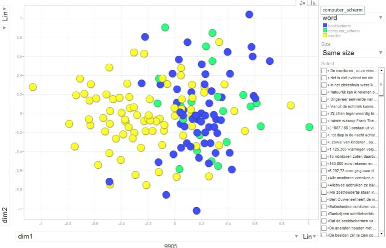
To illustrate the information that is avail-able through this visualization, we discuss the weighted chart for the concept COMPUTER SCREEN (Figure 1 shows a screen cap, but we strongly advise to look at the interactive version on the website). In Dutch, this concept can be ref-ered to with (at least) three near-synonyms, which are color coded in the chart: beeldscherm(blue),

computerscherm (green) and monitor (yellow). Each bubble in the chart is an occurrence (token) of one these nouns. As Figure 2 shows, roling over the bubbles makes the stretch of text visible in which the noun occurs (These contexts are also available in the lower right side bar). This usage-in-context allows the lexicologist to interpret the precise meaning of the occurrence of the noun. The plot itself is a 2D representation of the seman-tic distances between all tokens (as measured with a token-level SVS) and reflects how the synonyms are distributed over the “semantic space”. As can be expected with synonyms, they partially popu-late the same area of the space (the right hand side of the plot). Hovering over the bubbles and look-ing at the contexts, we can see that they indeed all refer to the concept COMPUTER SCREEN(See example contexts 1 to 3 in Table 2). However, we also see that a considerable part on the left hand side of the plot shows no overlap and is only popu-lated by tokens ofmonitor. Looking more closely

kuleuven.be/˜u0038536/committees) 6

(http://code.google.com/apis/chart/ interactive/docs/gallery/motionchart. html)

7_{Since we worked with synchronic data, we did not} use this feature. However, Motion Charts have been used by Hilpert (http://omnibus.uni-freiburg.de/ ˜mh608/motion.html) to visualize language change in

MDS plots of hand coded diachronic linguistic data.

at these occurrences, we see that they are instan-tiations of another meaning ofmonitor, viz. “su-pervisor of youth leisure activities” (See example context 4 in Table 2). Remember that our corpus is stratified for Belgian and Netherlandic Dutch. We can make this stratification visible by chang-ing the color codchang-ing of the bubbles toCOUNTRY

in the top right-hand drop-down menu. Figure 3 shows that the left-hand side, i.e. monitor-only area of the plot, is also an all-Belgian area (hov-ering over the BE value in the legend makes the Belgian tokens in the plot flash). Changing the color coding to WORDBYCOUNTRY makes this even more clear. Indeed the youth leader mean-ing ofmonitoris only familiar to speakers of Bel-gian Dutch. Changing the color coding to the variableNEWSPAPERshows that the youth leader meaning is also typical for the popular, working class newspapers Het Laatste Nieuws (LN) and

Het Nieuwsblad (NB) and is not prevelant in the Belgian high-brow newspapers. In order to pro-vide more structure to the plot, we also experi-mented with including different K-means cluster-ing solutions (from 2 up to 6 clusters) as color-codable features, but these seem not very infor-mative yet (but see section 6).

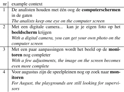
nr example context

1 De analisten houden met ´e´en oog decomputerschermen

in de gaten

The analists keep one eye on the computer screen

2 Met een digitale camera... kan je je eigen foto op het

beeldschermkrijgen

With a digital camera, you can get your own photo on the computer screen

3 Met een paar aanpassingen wordt het beeld op de moni-torennog completer

With a few adjustments, the image on the screen becomes even more complete

4 Voor augustus zijn de speelpleinen nog op zoek naar mon-itoren

For August, the playgrounds are still looking for supervi-sors

Table 2: Contexts (shown in chart by mouse roll-over)

detected by the lexicologist who can then report them to the computational linguist. The latter can then try to come up with a model that gives a bet-ter fit.

Finally, let us briefly look at the chart of another concept, viz. COLLISIONwith its near-synonyms

aanrijding andbotsing. Here, we expect the lit-eral collissions (between cars), for which both nouns can be used, to stand out form the figura-tive ones (differences in opinion between people), for which onlybotsingis apropriate in both vari-eties of Dutch. Figure 4 indeed shows that the right side of the chart is almost exclusively popu-lated bybotsingtokens. Looking at their contexts reveals that they indeed overwhelmingly instan-tiate the metaphorical meaning og collision. Yet also here, there are some “lost”aanrijdingtokens with a literal meaning and the visualization shows that the current SVS implementation is not yet a fully adequate model for capturing the words’ se-mantics.

6 General discussion

Although Vector Spaces have become the main-stay of modeling lexical semantics in current sta-tistical NLP, they are mostly used in a black box way, and how exactly they capture word meaning is not very clear. By visualizing their output, we hope to have at least partially cracked open this black box. Our aim is not just to make SVS out-put easier to analyze for comout-puter linguists. We also want to make SVSs accessible for lexicolo-gists and lexicographers with an interest in quanti-tative, empirical data analysis. Such co-operation brings mutual benefits: Computer linguists get ac-cess to expert evaluation of their models. Lexicol-ogists and lexicographers can use SVSs to iden-tify preliminary semantic structure based on large quantities of corpus data, instead of heaving to sort through long lists of unstructured examples of a word’s usage (the classical concordances). To our knowledge, this paper is one of the first at-tempts to visualize Semantic Vector Spaces and make them accessible to a non-technical audi-ence.

Of course, this is still largely work in progress and a number of improvements and extensions are still possible. First of all, the call-outs for the bubbles in the Google Motion Charts were not designed to contain large stretches of text. Cur-rent corpus contexts are therefore to short to

ana-lyze the precise meaning of the tokens. One op-tion would be to have pop-up windows with larger contexts appear by clicking on the call-outs.

Secondly, we didn’t use the motion feature that gave the charts its name. However, if we have diachronic data, we could e.g. track the centroid of a word’s tokens in the semantic space through time and at the same time show the dispersion of tokens around that centroid8.

Thirdly, in the current implementation, one im-portant aspect of the black-box quality of SVSs is not dealt with: it’s not clear which context features cause tokens to be similar in the SVS output, and, consequently, the interpreation of the distances in the MDS plot remains quite ob-scure. One option would be to use the cluster solutions, that are already available as color cod-able varicod-ables, and indicate the highest scoring context features that the tokens in each cluster have in common. Another option for bringing out sense-distinguishing context words was proposed by Rohrdantz et al. (2011) who use Latent Dirich-let Allocation to structure tokens. The loadings on these latent topics could also be color-coded in the chart.

Fourthly, we already indicated that two dimen-sional MDS solutions have quite high stress val-ues and a three dimensional solution would be better to represent the token-by-token similari-ties. This would require the 3D Charts, which are not currently offered by the Google Chart Tools. However both R and Matlab do have interactive 3D plotting functionality.

Finally, and most importantly, the plots cur-rently do not allow any input from the user. If we want the plots to be the starting point of an in-depth semantic analysis, the lexicologist should be able to annotate the occurrences with variables of their own. For example, they might want to code whether the occurrence refers to a laptop screen, a desktop screen or cell phone screen, to find out whether their is a finer-grained division of labor among the synonyms. Additionally, an eval-uation of the SVS’s performance might include moving wrongly positioned tokens in the plot and thus re-group tokens, based on the lexicologist’s insights. Tracking these corrective movements might then be valuable input for the computer lin-guists to improve their models. Of course, this

8

goes well beyond our rather opportunistic use of the Google Charts Tool.

References

Marco Baroni and Alessandro Lenci. 2011. How we BLESSed distributional semantic evaluation. In Proceedings of the GEMS 2011 Workshop on GE-ometrical Models of Natural Language Semantics, pages 1–10, Edinburgh, UK. Association for Com-putational Linguistics.

Samuel Brody and Mirella Lapata. 2009. Bayesian Word Sense Induction. InProceedings of the 12th Conference of the European Chapter of the ACL (EACL 2009), pages 103–111, Athens, Greece. As-sociation for Computational Linguistics.

Paul Cook and Suzanne Stevenson. 2010. Automat-ically Identifying Changes in the Semantic Orien-tation of Words. In Proceedings of the Seventh International Conference on Language Resources and Evaluation (LREC’10), pages 28–34, Valletta, Malta. ELRA.

Trevor Cox and Michael Cox. 2001. Multidimen-sional Scaling. Chapman & Hall, Boca Raton. Dirk Geeraerts. 2010a. The doctor and the

seman-tician. In Dylan Glynn and Kerstin Fischer, edi-tors,Quantitative Methods in Cognitive Semantics: Corpus-Driven Approaches, pages 63–78. Mouton de Gruyter, Berlin.

Dirk Geeraerts. 2010b. Theories of Lexical Semantics. Oxford University Press, Oxford.

Markus Gesmann and Diego De Castillo. 2011. Using the Google Visualisation API with R: googleVis-0.2.4 Package Vignette.

Dylan Glynn and Kerstin Fischer. 2010. Quanti-tative Methods in Cognitive Semantics: Corpus-driven Approaches, volume 46. Mouton de Gruyter, Berlin.

Thomas L. Griffiths, Mark Steyvers, and Joshua Tenenbaum. 2007. Topics in Semantic Represen-tation.Psychological Review, 114:211–244.

Kris Heylen, Yves Peirsman, Dirk Geeraerts, and Dirk Speelman. 2008. Modelling Word Similarity. An Evaluation of Automatic Synonymy Extraction Al-gorithms. In Proceedings of the Language Re-sources and Evaluation Conference (LREC 2008), pages 3243–3249, Marrakech, Morocco. ELRA. Thomas K Landauer and Susan T Dumais. 1997. A

Solution to Plato’s Problem: The Latent Semantic Analysis Theory of Acquisition, Induction and Rep-resentation of Knowledge. Psychological Review, 104(2):240–411.

Roeland J F Ordelman. 2002. Twente Nieuws Cor-pus (TwNC). Technical report, Parlevink Language Techonology Group. University of Twente.

Sebastian Pad´o and Mirella Lapata. 2007. Dependency-based construction of semantic space models. Computational Linguistics, 33(2):161–199.

Patrick Pantel and Dekang Lin. 2002. Document clus-tering with committees. InProceedings of the 25th annual international ACM SIGIR conference on Re-search and development in information retrieval, SIGIR ’02, pages 199–206, New York, NY, USA. ACM.

Yves Peirsman, Kris Heylen, and Dirk Geeraerts. 2008. Size matters: tight and loose context defini-tions in English word space models. InProceedings of the ESSLLI Workshop on Distributional Lexical Semantics, pages 34–41, Hamburg, Germany. ESS-LLI.

Yves Peirsman, Dirk Geeraerts, and Dirk Speelman. 2010. The automatic identification of lexical varia-tion between language varieties. Natural Language Engineering, 16(4):469–490.

Christian Rohrdantz, Annette Hautli, Thomas Mayer, Miriam Butt, Daniel A Keim, and Frans Plank. 2011. Towards Tracking Semantic Change by Vi-sual Analytics. In Proceedings of the 49th An-nual Meeting of the Association for Computational Linguistics: Human Language Technologies, pages 305–310, Portland, Oregon, USA, June. Associa-tion for ComputaAssocia-tional Linguistics.

Tom Ruette, Dirk Geeraerts, Yves Peirsman, and Dirk Speelman. 2012. Semantic weighting mechanisms in scalable lexical sociolectometry. In Benedikt Szmrecsanyi and Bernhard W¨alchli, editors, Aggre-gating dialectology and typology: linguistic vari-ation in text and speech, within and across lan-guages. Mouton de Gruyter, Berlin.

Eyal Sagi, Stefan Kaufmann, and Brady Clark. 2009. Semantic Density Analysis: Comparing Word Meaning across Time and Phonetic Space. In Pro-ceedings of the Workshop on Geometrical Mod-els of Natural Language Semantics, pages 104– 111, Athens, Greece. Association for Computa-tional Linguistics.

Hinrich Sch¨utze. 1998. Automatic word sense dis-crimination. Computational Linguistics, 24(1):97– 124.

Peter D. Turney and Patrick Pantel. 2010. From Fre-quency to Meaning: Vector Space Models of Se-mantics. Journal of Artificial Intelligence Research, 37(1):141–188.

Figure 1: Screencap of Motion Chart for COMPUTER SCREEN

Figure 3: COMPUTER SCREENtokens stratified by country