Some contributions to finite sample analysis in three econometric models

A thesis presented for the degree of Doctor of Philosophy

in Economics

at

the University of Canterbury Christchurch, New Zealand

by

J.N.

Lye ~

I

ABSTRACT

In the standard classical regression model the most commonly

used procedures for estimation are based on the Ordinary Least

Squares Method, which is justified on the basis of well known

finite-sample properties. However, this model consists of a number

of assumptions, such as, for example, homoskedastic, serially

independent and normally distributed disturbances and nonstochastic

regressors. By changing these assumptions in one way or another,

different estimating situations are created, in many of which the

OLS estimator may have no statistical justification at all.

Further, alternative estimation methods have often been justified

only on the basis of their asymptotic properties, although in

practice economists frequently have to base their statistical

analysis on a relatively small number of observations. This

suggests that the particular estimator to use in any situation

should be chosen on the basis of finite-sample considerations.

The analysis of finite-sample properties of commonly used

estimators in three well known Econometric models is the focus of

this thesis. In particular the three models considered are: the

limited-information simultaneous equations model, the nonnormal

linear regression model and the nonnormal limited-information

simultaneous equation model. The techniques used include the

derivation of the estimators' exact distribution and when this is

analytically intractable Monte Carlo methods are employed.

The limited-information simultaneous equation model is

evaluating many of the commonly used estimators, including the

two - stage least squares estimator, is presented. Secondly this

method is then used, and combined with Monte Carlo analysis, to

compare the distributions of the limited-information maximum

likelihood and two-stage least squares estimators in misspecified

simultaneous equations models. The result of this comparison

indicates the superior performance of the limited-information

maximum likelihood estimator over the two-stage least squares

estimator in both correctly specified and misspecified simultaneous

equations models.

Recently, models with possibly nonnormal distributed

disturbances have attracted more attention. For such models,

independence and uncorrelatedness of the disturbance terms are not

equivalent. Using the nonnormal regression model the statistical

consequences of distinguishing between independence and

uncorrelatedness are considered when the disturbances are Student-t

distributed. The results obtained demonstrate that the distinction

between the two assumptions is an important one and the

consequences of making the wrong assumption can be serious.

Consequently, specification tests are also presented which test for

uncorrelatedness versus independence in the elliptically symmetric

family.

The nonnormal limited-information simultaneous equation

model provides a relatively new area of analysis as there are few

published results available on the effects of nonnormal

disturbances in the limited- information simultaneous equation

separately in the other two models previously considered. However,

to narrow the range of possible models that can be examined,

attention is focussed only on the exactly-identified simultaneous

equation model. This model has a number of interesting features

when the reduced-form disturbances are normally distributed. These

features are illustrated and then comparisons are made with the

same model when the distribution of the disturbances is widened to

include. the Student-t family. In this case, as for the nonnormal

linear regression model, a distinction needs to be made between

independently distributed and jointly distributed disturbances.

The consequences of these different assumptions are shown to be

important; specification tests relating to this distinction are

ACKNOWLEDGEMENTS

There are a nwnber of people and organizations whose help

and support I would like to acknowledge with gratitude: my

supervisor, David Giles, for his overseeing of this thesis, for

providing comments on all individual chapters and for his

encouragement in the furtherance of my academic career; Dorian

Owen, for reading and commenting on numerous drafts of chapters;

Arnan U11ah, for providing many suggestions and comments that

improved the presentation and content of Chapter 5; Ray Byron, for

his comments on Chapter 5 in his role as discussant at the second

International Postgraduate Conference, Perth, November 1988; Robin

Harrison, for help in producing the graphs; Robert Davies, for

supplying me with a Fortran version of one of his algorithms that

was used in Chapter 6; Ian Coope, for suggesting and providing

nwnerous algorithms used; The University Grants Committee, and The

Reserve Bank of New Zealand, for providing financial support.

Thanks are also due to The Reserve Bank of Ne,,, Zealand for

providing financial assistance so I could attend the second

International Post-graduate Conference, Perth, November 1988, and

The Department of Economics, University of Melbourne, for providing

financial support so I could return to Canterbury University during

Summer 1989 to complete this thesis. I would like to thank Karilyn

Smith for her care in preparing the final typed copy, and for her

patience in deciphering many pages of untidy manuscript. Finally,

I would like to thank my parents for their financial and moral

CONTENTS

ABSTRACT

ACKNOWLEDGEMENTS

1 . INTRODUCTION 1.1

1.2 1.3

A General Overview

The Models And Objectives An Overview of the Chapters

2. PRELIMINARY DEFINITIONS 2.1 Introduction

2.2 Preliminary Mathematical and Statistical Definitions

2.3 Multivariate Normal, Multivariate Student-T,

PAGE

i

iv

1

4

9

12

12

Elliptically-Symmetric and Wishart Distributions 15

2.4 Note on Layout 21

3. KERNEL DENSITY ESTIMATION

3.1 Introduction 22

3.2 The Method 23

3.3 The Asymptotic Properties 26

3.4 Choosing the Kernel, Window Width

and Sample Size 28

CHAPTER

4. MONTE CARLO EXPERIMENTS -A DESCRIPTION OF METHODOLOGY

4.1

Introduction

4.2 Number of Replications and the Estimation of DF's, PDF's and Measures of Location and Dispersion

4.3 Generation of Random Numbers

4.4 Estimation of the Unknown Parameters of the Models

5. THE NUMERICAL CALCULATION OF THE DISTRIBUTION FUNCTION OF A BILINEAR FORM TO A QUADRATIC FORM WITH ECONOMETRIC EXAMPLES

6. 5.1 5.2 5.3 THE 6.1 6.2 6.3 6.4 6.5 6.6 Introduction Main Results Special Cases

LIML AND TSLS ESTIMATORS Introduction

The Estimators

Finite-Sample Properties of the TSLS and LIML Estimators: A Review

The Key Parameters in the Misspecified Canonical Distributions

Properties of the Misspecified Distributions Some Final Comments

CHAPTER

7. EXTENSIONS OF THE NORMALITY ASSUMPTION: A REVIEW

7.1 The Normal Assumption

7.2 Nonnorma1 lID Disturbances - The Effect on Gaussian-type Statistics

7.3 Robust Estimation Techniques

7.4 Multivariate Elliptically Symmetric Distributions

7.5 Jointly Distributed versus Independent Disturbances

8. THE LOCATION/SCALE MODEL WITH STUDENT-t OBSERVATIONS

8.1 8.2 8.3

8.4 8.5

Introduction

Lloyd's Best Linear Unbiased Estimators

Maximum Likelihood Estimators for Independent Student-t Observations

Joint versus lID Student-t Observations Some Final Comments

PAGE

98

101 107

111

117

123 125

CHAPTER

9. THE GENERAL LINEAR REGRESSION MODEL WITH STUDENT-t OBSERVATIONS

9.1 Introduction

9.2 Properties of Maximum Likelihood Estimators with Dependent Student-t Errors

9.3 Properties of Maximum Likelihood Estimators with Independent Student-t Errors

9.4

9.5

Joint Versus lID Student-t Errors Some Final Comments

10. THE NONNORMAL LIMITED-INFORMATION SIMULTANEOUS EQUATIONS MODEL

10.1 Introduction

10.2 The Exactly-identified Limited-Information SEM

10.3 Consequences of Misspecification

11. TESTING THE ASSUMPTION OF JOINTLY-DISTRIBUTED VERSUS INDEPENDENTLY-DISTRIBUTED NONNORMAL DISTURBANCES

11.1 Introduction

11.2 Tests of Normality

11.3 Extension to Testing the Normality Assumption in Regression Models

11.4 Testing for Jointness Versus Independence 11.5 Monte Carlo Experiments

11.6 Some Final Comments

PAGE

161

162

163 184 200

202

203 228

246

247

253 255 257

CHAPTER

12. SUMMARY AND CONCLUSIONS

12.1 Overview 12.2 Methods Used

12.3 Results and Conclusions Obtained 12.4 Some Further Issues

REFERENCES

APPENDIX A

APPENDIX B

PAGE

267 268 269 279

282

312

LIST OF TABLES

CHAPTER 6

5.1 Median and 1QR for L1ML and TSLS Estimators 5.2 Median and 1QR for L1ML and TSLS Estimators

CHAPTER 8

A A

3.1 The Variance of ~LB' Empirical Variance of ~ML' the

CRLB and the Degrees of Freedom Parameter, ~, in the

Student-t Approximation for the Distribution of

"

"

" A

3.2 _{The Bias of aML, the Variance of aLB and the}

4.1

4.2 4.3

A

Variance of a

ML

Adjusted for Bias

A(D) A(I)

The Actual and Assumed Variances of ~ML'

M

_OLS

"(D)

A(I)

The Bias of a

ML

and a

OLS

Median-Bias of Adjusted

~~~)

_{and aOLS Estimators} " (1) for the Cauchy Distribution

CHAPTER 9

3.1 3.2 3.3

4.1

4.2 4.3 "

Empirical and Asymptotic MSE's for

f3

ML

for N A

Empirical and Asymptotic MSE's for

f3

ML

for N

A

Empirical MSE's for

f3

_{TLS and Actual MSE's for b} for N = 20

Comparison of MSE's for

~~~)

and b for

N

= 20 Comparison of Empirical Variances for

~(D)

_ML with Asymptotic Variance

Empirical MSE's for b(l) for N = 20

of

~(1)

for K 2, N = 20 ML

1'.(1)

CHAPTER 10

1\

2.1 Points of the Distribution Function of a in the

Exactly Identified Limi~ed-Information SEM with

Normally-Distributed Reduced-form Disturbances,

a = 0.5 and 5.33 and various 02

1\

2.2 Points of the Distribution Function of a in the

Exactly-Identified Limited-Information SEM with

Reduced-form Disturbances Distributed as in (2.6),

a = 0.5 and 5.33 and various 02

1\

2.3 Points of the Distribution Function of a in the

Exactly-Identified Limited-Information SEM with

Reduced-form Disturbances Distributed as (2.12),

a = 0.5 and 5.33 and Various 02

3.1 Comparison of Median and IQR for Estimators IML(I)

and DML(I)

3.2 Comparison of Median and IQR for Estimators IML(D)

and DML(D)

2 2

3.3 Asymptotic Variances for l+a (DML-a) and l+a (IML-a)

02 02

when reduced-form disturbances are distributed as

(2.6) and (2.12)

3.4 Effect of using the wrong Limiting Distribution

for standardized

a

when errors are

Jointly-Distributed but are thought to be

Independently-Distributed

3.5 Effect of using the wrong Limiting Distribution

1\

for standardized a when errors are

Independent1y-Distributed but are thought to be

Jointly-Distributed

PAGE

206

213

222

230

232

236

239

CHAPTER 11

5.1 Results of Monte Carlo Experiments for Linear

Regression Models using 5000 Replications

5.2 Results of Monte Carlo Experiments for

Exact1y-identified Limited-Information SEM using 5000

Replications and Corresponding to data set 1

5.3 Results of Monte Carlo Experiments for

Exactly-identified Limited-Information SEM using 5000

Replications and Corresponding to data set 2

APPENDIX A

Table Al The Eigenvalues of (B1 -qB2) and their mul tiplici ties

Table A2 Components of the Eigenvectors

PAGE

261

264

265

313

LIST OF FIGURES

CHAPTER 3

PAGE

5.1 Comparison of Different Kernels for Cauchy 34

Distribution Using 100,000 Replications

5.2 Comparison of Different Kernels for Cauchy

Distribution Using 100 Replications 35

CHAPTER 6

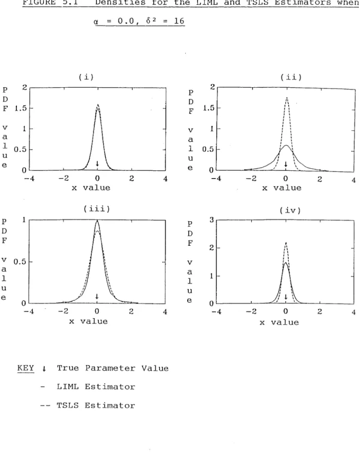
5.1 Densities for the LIML and TSLS Estimators when

2

0: = 0.0, {; = 16 87

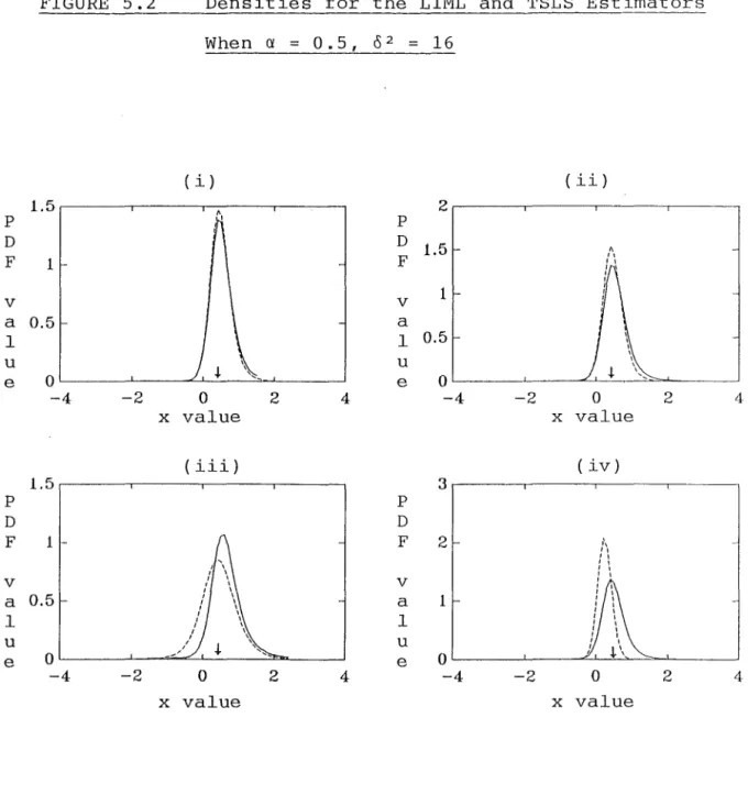
5.2 Densities for the LIML and TSLS Estimators when

2

0: = 0.5, {; = 16 88

5.3 Densities for the LIML and TSLS Estimators when

2

0: = 1.0, {; = 16 89

CHAPTER 7

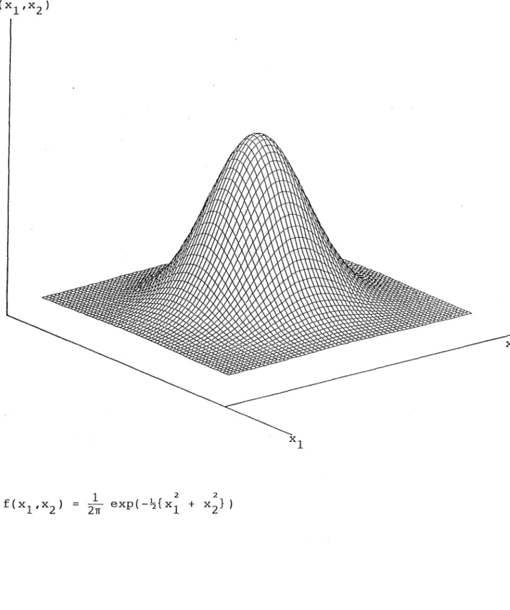
5.1 Bivariate Surface for Spherical Normal

Distribution 118

5.2 Bivariate Surface for Joint Spherical Cauchy

Distribution 119

5.3 Bivariate Surface for Independent Spherical

CHAPTER 8

PAGE

3.1 Comparison of Maximum Likelihood, BLUE and Student-t Approximation for the Standardized Location Parameter Corresponding to v = 3

and Different N l38

3.2 Comparison of Maximum Likelihood, BLUE, and Student-t Approximation for the Standardized Location Parameter Corresponding to Different

v and N = 10 139

3.3 Comparison of Maximum Likelihood and BLU Estimators for the Standardized Scale

Parameter 142

3.4 Comparison of Maximum Likelihood, BLUE and Student-t Approximation for the Standardized Location Parameter Corresponding to v = 1 and

N = 5 and 10 144

3.5 Comparison of Maximum Likelihood and Student-t Approximation for the Standardized Location

Parameter Corresponding to v = 1 and different N 145

3.6 Comparison of Maximum Likelihood and Student-t Approximation for the Standardized Location

Parameter Corresponding to v = 2 and different N 146

4.1 Distributions of

~(D)

_ML and

~(D)

_LB when the

Disturbances are Uncorrelated 152

4.2 _{The Distribution of MOLS for lID Student-t} "(I)

CHAPTER 9

3.1 Comparison of the Finite-Sample Distribution A

of ~ML. with its Asymptotic Distribution for

1

v = 3, N = 20

3.2 Comparison of the Finite-Sample Distribution A

of ~ML.with its Asymptotic Distribution for

1

v = 10,

N

= 20

3.3 Comparison of the Finite-Sample Distribution

4.1

A

of ~ML. with its Asymptotic Distribution for

1

v = 1, N = 20

Comparison of the distribution of

~(D)

_ML with its A(I) Incorrectly Assumed Asymptotic Distribution ~ML

for v = 3, N = 20

4.2 Comparison of the Distribution of b(I) with its Incorrectly Assumed Asymptotic Distribution beD) for v = 3, N = 20

4.3 Comparison of the Distribution of

~(D)

_{ML with its} Incorrectly Assumed Asymptotic Distribution A (I)

~ML

for v = 1, N = 20

4.4

Comparison of the Distribution of b (I) _{with its}

Incorrectly Assumed Asymptotic Distribution beD) for v = 1, N = 20

PAGE

176

177

178

187

191

196

CHAPTER 10

PAGE

2.1 Distributions of Maximum Likelihood Estimator in Exactly-Identified SEM with Normally Distributed

Reduced-form Disturbances Corresponding to a = 0.5 207

2.2 Distributions of Maximum Likelihood Estimator in Exactly-Identified SEM with Normally Distributed

Reduced-form Disturbances Corresponding to a = 5.33 208

2.3 Distributions of Maximum Likelihood Estimator in Exactly-Identified SEM with Student-t Distributed Reduced-form Disturbances given by (2.6) and Corresponding to a = 0.5

2.4 Distributions of Maximum Likelihood Estimator in Exactly-Identified SEM with Student-t Distributed Reduced-form Disturbances given by (2.6) and Corresponding to a = 5.33

2.5 Distributions of Maximum Likelihood Estimator in Exactly-Identified SEM with Student-t Distributed Reduced-form Disturbances given by (2.12) and Corresponding to a = 0.5

2.6 Distributions of Maximum Likelihood Estimator in

3.1 3.2

Exactly-Identified SEM with Student-t Distributed Reduced-form Disturbances given by (2.12) and Corresponding to a = 5.33

Graphs of DML(I) Graphs of IML(D)

215

216

224

CHAPTER 1

INTRODUCTORY COMMENTS

1.1 A GENERAL OVERVIEW

Consider the standard linear multiple regression model that

appears in all econometric textbooks (e.g. Johnston (1984), Harvey

(1981»:

y = X{3 + E (1.1)

where y' = (Y1" 'YN)' X is an N X K matrix, {3' = ({31" .{3K) is a

vector of unknown parameters and E' = (E

1 ... EN) is a vector of disturbances, and where the following conditions are satisfied:

Condition (i) : X is a nonstochastic matrix of rank K

<

N

and has the property that

(X' X)

lim

N

= Q,

N:>oo

where Q is a finite nonsingu1ar matrix. It is further assumed that there are no variables wrongly included in and/or excluded from the

X matrix.

Condition (ii) : E has a multivariate normal distribution with mean

O an d covar~ance · matrlx . a . 21

The most commonly used procedures for estimation and

inference in this model are based on the Ordinary Least Squares

(OLS) principle. This principle is justified on the basis of its

well known finite-sample properties which are given in Properties

Properties 1.1

(i) The least-squares estimator b = (X'X)-lx'y, which is also

the maximum likelihood estimator, and the associated

variance estimator s2 (y-Xb)' (y-Xb)/(N-K), are unbiased

minimum variance estimators from within the class of all

unbiased estimators.

(ii) The joint distribution of b is multivariate normal with mean

(iii)

(iv)

f3

and variance covariance matrix a2 (X' X) -1, implying that the marginal distribution for an element of the b-vector,

2 -1

and variance a (X' X) ... JJ b., is normal with mean

f3.

J J

say

The statistic (N-K)s 2

/a

2 is distributed as a chi-square random variable with N-K degrees of freedom.

Under the null hypothesis

f3

_j 0, the test statistic

~ 2 -1

b. / s (X' X) ..

J JJ has a Student-t distribution with N K degrees of freedom.

However, this model is not sufficient as a basis for

modelling many economic data generation processes, simply because

in many situations conditions (i) and (ii) do not hold. Consequently, Properties 1.1 are not valid in general and, in

particular, the use of OLS techniques may have no statistical

justification at all. The relaxation of these conditions has

enriched the range of econometric models and has consequently led

to the development of a number of estimation and inference

techniques which are alternatives to those based on OLS. The

introduction of most of these techniques however has only been

justified on the basis of their asymptotic properties, asymptotic

economists frequently have to base their statistical inferences on

a relatively small number of sample observations. This suggests

that the choice of the appropriate techniques to use should be

based on finite-sample considerations such as those given in

Properties 1.1, rather than asymptotic behaviour. However, in

general, relatively little is known about these relevant

finite-sample considerations.

The objective of this thesis is to extend and develop

finite-sample results for various estimators used for estimation

and inference in three econometric models. The particular

econometric models chosen are well-known extensions of the standard

multiple linear regression model when conditions (i) or (ii) or a

combination of both conditions are relaxed. Further, each of the

econometric models chosen provides a basis for much applied

econo-metric analysis and, in particular, all of the estimators

considered are now included in standard and widely-used econometric

packages such as SHAZAM and TSP.

The next section describes the three econometric models

chosen for investigation and so defines the three main components

of this thesis. These models are: the limited-information

simultaneous equations model, the nonnormal linear regression model

1.2 THE MODELS AND OBJECTIVES

(i) The Limited-Information Simultaneous Equations Model

Econometric models typically consist of sets of equations

which incorporate feedback effects from one variable to another.

These are known as Simultaneous Equation Models (SEMS). In

particular, when the econometrician is interested only in making

statistical inferences about the parameters of a single equation of

the model, then this is known as "The Limi ted- Information SEM".

Writing this model in the form of (1.1) implies that some of the

regressors in X are stochastic and are correlated with the

disturbance vector €, in the sense that (l/N)X'€ does not tend to

the zero vector as the sample size, N, tends to infinity.

Therefore condition (i) is invalidated, and furthermore OLS is an

inconsistent estimation technique.

The SEM was first proposed by Haave1mo (1943, 1944, 1947)

and this suggestion provided the basis for a research programme

undertaken by the Cowles Foundation during the late 1940' sand

early 1950's. However, the estimators suggested, such as Two Stage

Least Squares (TSLS) and the Limited Information Maximum Likelihood

estimator (LIML) , are rather complicated functions of the

underlying random variables, so that the exact distributions are

difficult to derive. Nonetheless, the analysis of the exact

distributions and their moments began in the early 1960' s and in

recent years substantial progress has been made for the case when

all of the predetermined variables are assumed to be exogenous and

the equation is identified by means of zero res tric tions (e. g.

1973b, 1977); Hillier, Kinal and Srivastava (1984); Hillier (1985);

Phillips (1980a, 1980b, 1984a, 1984b, 1985); Anderson (1982».

the finite-sample properties of certain Although

test-statistics and variance estimators have received some

attention in the literature, most results are concerned with the

estimation of the parameters of the structural equation of interest

and, in particular, the coefficients of the endogenous regressors.

It is this topic that is pursued here.

Traditionally a distinction is made between models in which

the structural equation of interest contains only one endogenous

regressor, and more than one endogenous regressor. This is because

it is only recently that techniques have been developed which allow

for the derivation of the exact densities in the case of more than

one endogenous regressor, and even then these results are complex

and currently not suitable for numerical evaluation.

Consequently, most numerical evaluations have concentrated simply

on the one endogenous regressor case. One of the themes in this

case has been the numerical comparison of the distributions of the

LIML and TSLS estimators. In particular the numerical computations

of Anderson et al. (1979, 1982) have pointed to the superior

performance of the LIML procedure over the TSLS estimator. In this

thesis this analysis is extended to the comparison of the

distributions of the TSLS and LIML estimators when there are

predetermined variables wrongly included in and/or excluded from

the model.

The numerical procedures used in this thesis differ from

those of Anderson et al. (1979, 1982). In particular, as most of

as a ratio of quadratic forms in normal variables it is shown how

the techniques such as those developed by Imhof (1961) and Davies

(1973) can be used to compute the distribution functions. This is

an extension of the analysis in Cribbett et al. (1989) which

concentrates only on the TSLS estimator. In the case of the LIML

estimator, however, the nonparametric density estimator is

integrated with a simple Monte-Carlo approach to estimate the

density, due to the complexity of numerically evaluating the exact

expressions.

(ii) The nonnormal linear regression model

When it is assumed that the error distribution is nonnormal,

condition (ii) is invalidated. In the literature a distinction is

commonly made on the basis of whether the distribution has a finite

or infinite variance.

If the error distribution is assumed to have finite first

and second moments then the properties of OLS are well-known. The

OLS estimator of ~ is best linear unbiased (BLUE) and the

conventional tests are asymptotically justified in the sense that

they have the correct size asymptotically. These results have

often been the justification for the use of the least squares

estimator under conditions of nonnormality. However, there are two

problems with this approach. First, it is well-known that although

OLS is BLUE it is, in general, asymptotically inefficient.

Consequently there may be nonlinear estimators which have superior

finite and asymptotic properties. Secondly, there is a large body

of literature (e.g. Mandelbrot (1963a, 1963b, 1966), Fama (1963,

particularly prices in financial and commodity markets, are well

represented by a class of distributions with infinite variance. A

distribution with an infinite variance has "fat tails" which

implies that large values or "outliers" will be relatively

frequent. Because the least squares technique minimizes squared

deviations, it places relatively heavy weight on outliers, leading

to estimates that are extremely sensitive to the presence and

values of such observations.

In recent years, to broaden the assumption of nonnormality

in the linear regression model, it has often been assumed that the

error components follow a joint multivariate elliptically symmetric

distribution. Under this assumption it has been shown that the

resulting estimators and test statistics possess properties which

make them analytically tractable and, furthermore, in many cases,

identical to those obtained under the normality assumption. See,

for example, Zellner (1976), King (1979, 1980), Singh (1987, 1988).

However, the normal distribution is the only member of the

class of multivariate elliptically symmetric distributions where

the disturbances are, in fact, independent. Also, it is usually

forgotten that the marginal distributions of the disturbance terms

under this assumption are identical to those obtained when the

disturbances are assumed to be independently and identically

distributed (iid) elliptically symmetric. It is these features

that lead naturally to the question of the statistical consequences

of distinguishing between multivariate and iid elliptically

symmetric error distributions and it is this issue that is taken up

Kelejian and Prucha (1985) address this problem using

asymptotic criteria for the linear regression model and Student-t

errors for degrees of freedom greater than 2. This distribution is

a particularly important member of the elliptically symmetric class

because it is claimed by authors such as Judge et al. (1985) that

this distribution may be a reasonable way of modelling tails that

are fatter than those of the normal distribution. (see also the

recent article by Lange et al. (1989)). The obj ective here is to

extend this analysis by developing properties of the maximum

likelihood estimators for the entire Student-t family using

finite-sample criteria. Results are obtained assuming the data

matrix, X, is nonstochastic.

(iii) The Nonnormal Limited-Information Simultaneous Equations Model

Models (i) and (ii) can be related by simultaneously

relaxing both of the conditions associated with the standard linear

regression model. This model provides a relatively new area of

analysis as there are few published results available on the

effects of nonnormal disturbances in the limited- information SEM

(e.g. Knight (1985b, 1986), Raj (1980), Donatos (1989)).

The objective here is to combine both of the themes pursued

separately in Models (i) and (ii). In particular, in the

estimation of the coefficient of the one endogenous regressor in

the exactly-identified limited-information SEM, the statistical

consequences of distinguishing between multivariate and iid.

Student-t error distributions on the LIML and TSLS estimators are

examined. Although (because it is exactly-identified) it is a

number of interesting features when the errors are normally

distributed. In particular, in this case the TSLS, LIML and Least

Variance Ratio (LVR) estimators are identical and

1

distribution is bimodal over part of the parameter space.

1.3 AN OVERVIEW OF THE CHAPTERS

their

Chapter 2 reviews certain key concepts in probability and

statistical inference used in this thesis. It also introduces the

notational conventions used.

Chapter 3 reviews an essential tool of analysis that is used

throughout this thesis. This is the integration of the

nonparametric density estimator with the Monte-Carlo technique.

This is a useful technique for approximating many of the density

functions considered in the thesis when either the exact

distribution is too difficult to derive explicitly or when the

exact distribution is known but too complex to be analyzed

conveniently. A number of statistical properties of this estimator

are discussed. These are all asymptotic properties, but are

considered relevant because in the applications considered here,

sample size, which is simply the number o( replications in the

simulation experiment, can be chosen by the investigator.

Chapter 4 discusses the methods used in the simulation

experiments. In particular, this includes a discussion of the

choice of the number of replications in the simulation experiments,

the generation of the random numbers involved, and the algorithms

used to solve the likelihood equations associated with the models

considered.

Chapter 5 shows that the exact distribution of a ratio of a

bilinear form to a quadratic form in normal variables can be

computed using techniques such as those developed by Imhof (1961)

and Davies (1973). As many of the commonly used estimators in the

limited-information SEM, including TSLS, are of this form, this is

a useful technique for the numerical evaluation of their

distributions.

Chapter 6 reviews recent relevant finite-sample properties

in the literature on the limited-information SEM. It also pursues

the theme of comparing the LIML and TSLS distributions, which

involves the use of techniques discussed or developed in Chapter 3

and Chapter 5.

Chapter 7 reviews some alternatives to the assumption that

the disturbances in the econometric models considered are

distributed normally. In particular, the effects of iid

nonnorma1ly distributed regression disturbances on the traditional

inference and estimation procedures used for normally distributed

disturbances are discussed, and a class of alternative estimation

techniques collectively labelled "robust estimators" are reviewed.

Also in this chapter, the consequences of replacing the normality

assumption with the assumption that the regression disturbances

follow a multivariate elliptically symmetric distribution are

examined. Therefore two types of nonnorma11y distributed

disturbances are reviewed in this chapter, these being, iid

nonnormal1y distributed disturbances and multivariate distributed

chapters. That is, "an examination of the statistical

conse-quences of distinguishing between the regression disturbances

following a multivariate elliptically symmetric distribution and an

iid elliptically symmetric distribution".

Chapters 8 and 9 take up this theme in the nonnormal linear

regression model. Chapter 8 considers the "location-scale" model,

which is a special case of the linear regression model. It is

equivalent to only estimating the intercept term in the linear

regression model. Chapter 9 extends the results obtained to the

more general model. A distinction is made between the

location-scale model and the more general model simply because a

number of techniques can be used to examine the problem in the

location-scale model that do not generalize to the more general

model.

Chapter 10 pursues this theme in the exactly-identified

nonnorma1 limited-information SEM. In particular, the

distributions of the TSLS and LIML estimators are compared, since

with nonnorma1 disturbances these two estimation techniques are not

necessarily the same.

Chapters 8, 9 and 10 indicate the importance of making the

distinction between iid nonnormally distributed disturbances and

multivariate nonnormally distributed disturbances. This suggests

that it is important to construct appropriate specification tests

that make this distinction. This is the topic of Chapter 11.

Finally, Chapter 12 offers some conclusions and presents

CHAPTER 2

PRELIMINARY DEFINITIONS

2.1 INTRODUCTION

The purpose of this Chapter is to introduce the notational

conventions used throughout this thesis.

Section 2.2 defines preliminary mathematical and statistical

definitions, such as those given in De Groot (1970), Feller (1966,

1968) and Muirhead (1982). Section 2.3 defines a number of

distributions that are used throughout this thesis. These include

the multivariate normal, multivariate Student-t, multivariate

elliptically-symmetric and Wishart distributions. Finally, Section

2.4 gives a brief note on the layout of the thesis.

2.2 PRELIMINARY MATHEMATICAL AND STATISTICAL DEFINITIONS

(i) Random Variables

A probability space is defined as the combination (0, A, P)

where, 0 is a set of points, A is a a-field of subsets of 0, and P

is a probability distribution defined on the elements of A.

1

Furthermore, any set LEA is known as an event.

A random variable Z is a real valued function from 0 to the

real line R which satisfies the condition that for each Borel set B

E

fi

on R, the set Z-l(B) = (W:Z(W)EB,WEO) is an event in A.

A collection of random variables Zl(w),Z2(w)", on a given

pair (O,A) will be denoted by Zl' Z2' ... A random vector is a

K-tuple ZK = (Zl" ,ZK) of random variables defined on a given pair

(O,A) .

No distinction will be made between a random variable or

vector and the value taken by that random variable or vector.

(ii) Distribution, Probability Density and Characteristic Functions

Associated with a random vector ZK on (O,A,P) is a distribution function defined on RK by

FK(tl · .. t K) = Pro ((W:Z1 (W)

~

t 1 .. ,ZK(w) ~ t K} ) (2.1)

K

for all t E R . The joint distribution of Zl" ,ZK is absolutely

continuous if there exists a nonnegative joint probability density

K

function pdfK(Zl" ,ZK) such that for every Borel set B cR.

(2.2)

The characteristic function of a random K-vector ZK is defined as

-1. (2.3)

The characteristic function always exists and no two different

distributions yield the same characteristic function so that there

is a one-to-one correspondence between characteristic functions and

(iii) Marginal Distribution Functions

The j oint distribution of a subset of random variables Zl ... Zp of Zl ... ZK (p ~ K) is called a marginal distribution.

marginal j oint distribution F of Zl ... Z is determined from the _{p p} The

joint distribution function by the relation

(2.4)

p+1. .. K

Similarly, the marginal j oint probability density function pdfp of Zl ... Zp is determined from the joint probability density function pdfK Zl ... ZK by the relation

pdfp (Zl·· .Zp) =

J

K~~

J

pdfK(Zl·· .ZK)dZp+_{1 ·· .dZK· (2.5)}

R

Let G. denote the marginal univariate distribution function ~

of the random variable Z ..

~ The random variables Zl ... ZK are independent if and only if (iff) their joint distribution function can be factored at every point (Zl ... ZK) E RK as follows:

(2.6)

(iv) The Expectation Operator

The expectation E(Z) of any random variable Z with distribution function F is defined as

E(Z) =

J

Z pdf(Z)dZ

R1

and it exists iff the integral exists.

(2.7)

mean of Z or the expected value of Z. For a random vector ZK the mean is defined as

(2.8)

The variance of a random variable Z is given by E[(Z-E(Z»)1 and denoted var(Z). The covariance between random variables Zl and Z2 is defined as [(Zl-E(Zl»)(Z2-E(Z2»] and denoted cov(Zi,Zj)' Equivalently, this can be expressed as

For a vector ZK' the covariance matrix is ~ = (aij)KxK' where aij

cov(Z.,Z.).

~ J

2.3 MULTIVARIATE NORMAL, MULTIVARIATE STUDENT-T, ELLIPTICALLY-SYMMETRIC AND WISHART DISTRIBUTIONS

(i) Multivariate .. Normal and Student-t distributions

A K-dimensional random vector ZK has a nonsingular normal distribution with mean J.L

K

and covariance matrix ~ if ZK has an absolutely continuous distribution whose probability density function

pdf(ZKIJ.LK'~)

is specified at any point ZK E RK by the equation

(3.1) In (3.1) J.L

components can be arbitrary real numbers and ~ must be a symmetric

and positive definite matrix. This distribution is denoted

-1

~

.

Define the precision matrix T of NK (JL!~:~) to be equal to

Suppose that Y

K is NK(JLK'~) with precision matrix T and

suppose the random variable

i

is distributed independently of Y

and is chi-square distributed with v degrees of freedom, so that

2

pdf(X ) =

where r(a) is the gamma function,

r(a)

f

x a-1 exp(-x)dx, a

>

0

o

If the components of ZK are defined by the equation,

1

2 2

Z. = y.(K)

+

JL. , i = l ... K, 1. 1.V 1.

(3.2)

(3.3)

(3.4)

with v then the distribution of ZK is multivariate Student-t,

degrees of freedom, location vector ILK and precision matrix T. It

is denoted by MTK(ILK,T,v), and the probability density function of

Z E RK .

K

1.S,

r

r

1

_ (v+K)

For v

>

1, the mean vector E(Z~) = p,~ exists, and for v

>

2 the

covariance matrix exists and is equal to _v-v2~'

In both cases the marginal distributions are easy to derive.

Suppose that the random vector Z~ is partitioned in the form,

ZK

~ [:~

1

)~

where the dimension of Zi is Ki (i = 1,2) and Kl + K2 K. Also

suppose that p,~, T and ~ are partitioned as

T

[

~ll

~21 ~12

~22

1 '

where the dimension of p,. is K. (i = 1,2) and the dimension of the

1. 1.

sub- matrices T .. and ~ .. is K. X K. (i,j = 1,2).

1.J 1.J 1. J K

normal distribution at any point

Z~

E R 1 the value

~l

Then, for the

*

pdfK (Zl) of

1

the marginal probability density function of Zl is specified as

~l

For the multivariate Student-t distribution it is,

-1

where T* = Tll - T12T22T2l' Therefore, in both cases, the marginal distributions are members of the same family as their respective joint distributions.

Further properties of both of these distributions can be found in, for example, De Groot (1970, pp.50-60).

Elliptically Symmetric Distributions

Each of the distributions above belong to the wider family of multivariate elliptically-symmetric distributions. The random vector ZK has a multivariate elliptically-symmetric distribution if the characteristic function ~Z _ (sK) of (Z_K - ~_K) is a function

K

J-l

K

-of the quadratic form sKh sK' (where sK is a row vector), that,

such

(3.8)

for some function

1/1.

If it is further assumed that the density function with nonsingular h exists, then it is of the form,

1

where g is a one-dimensional real-valued function independent of K

and CK is a scalar proportionality constant. This distribution is

denoted MES(~,T) and it has the first two moments, E(Z~) = ~K and

Cov(Z~) = a~, where a = -2~' (0), provided these moments exist. If

~ = 0 and ~ = I in (3.8) then the multivariate elliptically

~

symmetric distributions are called spherically symmetric

distributions. Two properties of these distributions used in this

thesis are (see, for example, Muirhead (1982, p.34»:

Properties 3.1

(1) All marginal distributions are elliptical and all marginal

density functions of dimension p ~ K have the same

functional form.

(2) If Z~ is N(~~,~) and ~ is diagonal then the components

Zl' .. ZK of Z~ are all independent. Wi thin the class of

multivariate-elliptically symmetric distributions

independence when ~ is diagonal characterizes the normal

distribution.

Further properties of these distributions are discussed by

authors such as Chmielewski (1981), Kelker (1970), King (1979),

Cambanis, Huang and Simons (1981) and Muirhead (1982).

(iii) The Wishart Distribution

The Wishart distribution is used in the derivation of

limited-information simultaneous equations models (as discussed in Chapters 5 and 6). The Wishart distribution is a matrix generalization of the noncentral chi-squared distribution (see, for example, Johnston and Kotz (1972, p.158». Consider the random n x

K matrix

Z

Z'

₁

Z'

_n

where the Z. terms are independent normal random vectors with mean

1.

M. and covariance matrix E.

1. The K

x

K matrix W = Z'Z, with (i,j)th

element Z(i),z(j), is said to be a Wishart matrix. The elements of W have a non- central Wishart distribution of order K, with n degrees of freedom, covariance matrix E and noncentrality parameter

n

M = E MiMi, This is denoted by i=l

The distribution is said to be central if M = O.

(3.10) The Wishart distribution has properties similar to those of the noncentral chi-squared distribution. In particular, if A and B are symmetric idempotent matrices, then Z'AZ - WK[q,E,E(Z)'AE(Z)], where q is the rank of A, and Z'AZ and Z'BZ have independent Wishart distributions

2.4 NOTE ON LAYOUT AND NOTATION

The purpose of this chapter has been to introduce the basic

notational conventions used in this thesis. Other notation used

that is not introduced in this chapter is defined when it is

required.

The layout of this thesis is as follows. Each chapter is

divided into sections. Theorems, Equation Numbers, Properties and

Figures within each section of a chapter are denoted by their

section number and then in sequence. Therefore, when referenced in

other chapters they are denoted by their chapter number first and

CHAPTER 3

KERNEL DENSITY ESTIMATION

3.1 INTRODUCTION

There are a number of techniques that are used to

approximate density functions, either when the exact distribution

is too difficult to derive explicitly, or when the exact

distribution is known but too complex to be analyzed conveniently.

For example, the exact sampling distributions of estimators of the

unknown coefficients of the endogenous variables in single

structural equations, have been shown to depend upon multiple

infinite series of zonal-type polynomials, and these present

enormous difficulties in numerical work. Phillips (1980a, 1983)

has overcome these difficulties by extracting various j oint and

marginal density approximations using asymptotic expansions.

However, another method which may be used to analyze such

distributions is the Monte Carlo method, in which artificial data

are generated and from them sampling distributions and moments are

estimated. One advantage of this technique is that it can be

implemented easily on an extensive range of models and error

probability distributions. An extension of this technique which is

used in this thesis is the integration of density estimation with

the Monte Carlo technique, as suggested by Ullah and Singh (1985).

That is, the Monte Carlo approach is used to generate the

statistics of interest and then the density of these statistics is

estimated using the generated statistics as observations. The

obj ective of this chapter is to briefly review the history and

is a particular example of a density estimator that is both widely

used and thoroughly studied in the statistical literature. The

actual Monte Carlo methodology that is used in this thesis is the

topic of the next chapter.

The Kernel estimation technique has been reviewed by, for

example, Tapia and Thompson (1976), Singh, Ullah and Carter (1987),

Wertz (1978), Devroye (1987), Silverman (1986), and Ullah (1988)

and the contents of this chapter draw heavily on these reviews.

The finite-sample analysis of statistics is the application of the

Kernel density estimation technique that will be used throughout

this thesis. Recently there has been a great deal of interest in

other applications of the technique, such as applying the method to

the estimation and testing of econometric models. A review of

these applications is beyond the scope of this chapter. However,

these applications have been reviewed by Bierens (1986), Singh

et al. (1987) and Ullah (1988).

In Section 2 the Kernel density estimation technique is

defined and its history is briefly reviewed. Section 3 considers

the asymptotic properties of this estimator and Section 4 considers

the choice of Kernel, window width and sample size.

concludes this chapter with a simple illustration.

3.2 THE METHOD

Section 5

Let _{Xl ,X2 , ... ,XN}

*

be independently and identically

distributed observations on a random variable X with probability

density function pdf (X) . Rosenblatt (1956) and Parzen (1962)

pdf(X) 1 N* [X-X.] l:: K J j=l h(N~'<')

(2.1)

where h(N*) is the window width, which is assumed to be a positive

function of the sample size, N*, such that lim h(N*) = 0, and K is

N~C()

the Kernel. If K is everywhere a nonnegative function and

satisfies

J

K(x)dx 1, then pdf(X) will be a probability density

function which possesses

all

of the continuity and

differentiability properties of K. Numerous extensions of this

estimator have been considered. For example, Breiman et a1. (1977)

introduced the variable Kernel estimator in which the window width

varies across the data points, allowing the tails of the estimator

to be smooth while not distorting the central part of the density.

Cacou11os (1966 ) extended the Kernel estimator to the

estimation of multivariate density functions. Let

Xi = x(xii) X(i) ₂

...

x~i))

i 1

.

..

N*

be a given sample of N* independent realizations of an

m-dimensiona1 random variable X(X1 X) from a population _m

characterized by a continuous m-variate probability density f(X1

... X). The estimator suggested by Cacou11os is, _m

pdf(X)

(2.2)

where (as in the univariate case), h(N~'<') is the window width,

assumed to be a positive function of sample size such that

lim h(N*)

N*:;.oo 0, and K is the natural generalization of the

univariate Kernel. This estimator uses only a single h(N*) for all

appropriate (see, for example, Ullah (1988, p.634». On occasions throughout this thesis an estimate of the appropriate marginal density is required, and these can be estimated using the expression in (2.2). Conditional densities can also be estimated; however, the details will not be given here but can be found in Ullah (1988).

Suppose that the vector of realizations is written as,

Xi(Xii)

x~i)

.,.

x~i))

= xi(z(i) ,y(i»)

where Z(i) is a p X 1 vector and y(i) is a q X 1 vector such that p

+ q = m. The marginal density of Zt at Z is

J

p~f(Z,y)dy

(2.3)

One example of a joint Kernel K from which marginal densities can be found easily is studied by Epanechnikov (1969), and is given by the equation

pdf(X) N*-l L: N~~ m II

t=l i=l

If each Ki satisfies

J

Ki(x)dx can be written as,

_1_ K 1. 1.

[

X.

-X~

t)]

h (N*) i h (N*) . (2.4)

1 and h. (N*) _1. h(N*), then (2.3)

N~~ q

N*-l L: h(N*)-q II

K

[

z._z~t)]

J J

j h(N*) . (2.5)

t=l j=l

In particular, when (2.4) and (2.5) are used in this thesis it is assumed that each K. has the same form, such as, for example, K. _{1. 1.} __

1_exp(_~y2),

the normal Kernel.

3.3 THE ASYMPTOTIC PROPERTIES

The asymptotic properties of the Kernel estimator are

particularly relevant for the application of the density estimation

technique to the finite-sample analysis of statistics. This is

because the sample size, N*, which is the number of replications of

the simulation experiment, can be chosen and is bounded only by the

limits of the duplication of the random number generator. The

obj ective of this section is to present some of the asymptotic

properties of Kernel estimators. In particular, these properties

are dependent upon the chosen Kernel, window width and the unknown

density. A more extensive review can be found in Ullah (1988,

pp.638-642).

To obtain these asymptotic properties, certain regularity

conditions are specified on the Kernel, window width and density.

The following set of assumptions are taken from Ullah (1988,

p.639). Let K be the class of Borel-measurable bounded real valued

functions K(x), x = (xl" .xm) such that for the:

Kernel

I. (i) J K(x)dx = 1

(ii) JIK(X)ldX

<

00

(iii) IIxllmIK(x) I=}O as II xII =} 00 where II

.11

is the Euclidean norm.

(iv) supIK(x)1

<

00.

Window Width

II.

h(N*) =} 0 as N*=} 00

Density

IV.

pdf(x) is continuous at any point xO'

Using these assumptions Cacoullos

(1966)

has shown that if

I, II

and

IV

hold,

lim E

[P~f(X)]

= pdf (x)

N*=}ex:>

which implies pointwise asymptotic unbiasedness, and if

I, II,

III

and

IV

hold,

1\ p

pdf(x) =} pdf (x) as N* =} ex:>

at any point and therefore implies pointwise weak consistency. Other results have also been shown to hold. For example, Deheuvels

(1974)

develops weaker conditions under which these results hold, and Devroye and Wagner

(1976)

develop strong consistency results assuming some further conditions.

Each of the properties above are pointwise properties. Some authors (e.g. Bai and Chen

(1987»

have obtained results for global properties, using criteria such as those based on the norm Lp, which involve considering conditions under which

[J

1\ ] lip

Ipdf(x) - pdf(x)IPdx _=}

°

_{as N*}

(3.1)

The last asymptotic property to be discussed is the property of asymptotic normality, which is useful for deriving confidence intervals for pdf(x). The results of Parzen

(1962)

and Cacoullos

(1966)

imply,

1

(N*hm(N*»)2[P~f(X)

-

E(P~f(X»)]

- N(O,Pdf(X)JKZ) (3.2)

1

(N*hm(N*»)2Bias[p~f(X)]

tends to zero asymptotically since,

1

(N*hm(N*»)

2[P~f(X)

- pdf (x) ] = (N*hm(N*»)

[P~f(X)

- E

(P~f(X»)]

1

+

(N*hm(N*»)2Bias[p~f(X)]

Ullah (1988, p.642) shows that This implies that asymptotically then (3.2) holds.

Bias

[P~f(X)]

is 4+m

if N*h-2-(N*)

(3.3)

proportional to tends to zero

As an example, consider the univariate normal Kernel 1 1 2

--exp( --y ), then the 99% asymptotic confidence interval for

v'2ii

2

pdf (x) is given by

1

pdf(x) ± 2.58 (3.4)

3.4 CHOOSING THE KERNEL, WINDOW WIDTH AND SAMPLE SIZE

In the implementation of the Kernel estimator and in the use of the results in the previous section, the selection of h, K and N* is required. Most emphasis in the literature has been given to choosing a suitable window width and Kernel on the basis of minimizing some measure. The usual measures to be taken are approximate bias, mean squared error (MSE) , or integrated mean squared error (IMSE) of pdf(x) where,

(4.1)

is used as a global accuracy measure of f as an estimator of f.

The approximations to these measures are obtained using similar

me thods to Kadane' s (1971) small disturbance expansion of

estimators, and they can be found in Ullah (1988, p. 642) . The

existence of these approximations require a number of assumptions

as given in Ullah (1988, p.64l).

The optimal h that minimizes MSE is,

-1/(m+4)

h* = cN*

,

. where

,

(4.2)

[ { }

2 ] -1/m+4

c = mpdf(x) Dpdf(x)

J

x 2K(x)dx

J

K2(x)

and for IMSE is,

h* c*N*-1/(m+4); where, _(4.3)

d 2pdf(x)

where Dpdf(X) is the operator 8x8x' , so that h* converges to 0

as

N*~ ~

but only at the rate N*-1/m+4.

However, these choices are not in general operational as

they depend upon the unknown dens i ty . However, suitable

operational window widths have been suggested which depend upon the

actual estimator pdf(x). Simply, in (4.2) and (4.3) above, pdf(x)

replaces pdf(x), and the iteration process is begun with an initial

arbitrary starting value for h. However, the rate of convergence

of this estimator may be slow (see, for example, Ullah (1988,

p.644».

There are various other ways of choosing h. The

cross-validity approach is one that has often been used. It is

and it involves a completely data- based choice for h. There have

been a number of papers that have examined the asymptotic

equivalence of the cross-validity choice to MISE (e.g., Hall

(1983), Stone (1984».

Tapia and Thompson (1976) suggest an "interactive" method

which is useful mainly in the univariate case. It is recommended

that the estimation technique begins with h values that are too

large, that is, when the pdf is obviously overly smoothed, and then

h is sequentially decreased until overly noisy probability density

estimates are obtained. The point where further attempts to

improve resolution, by decreasing h lead to noisy estimators is

generally fairly sharp and readily observable. Examples of this

approach are given by Tapia and Thompson (1976, pp.61-66).

Alternatively, they also present an empirical algorithm which

iterates according to the algorithm:

[

I

2 ] -1/5

[1\

]

-1/5

h. = N*-1/5K (x)dx JIDPdf(x)1 2dX

1+1 Ix2K(x)dx

Other approaches have been suggested and the details are

given in U11ah (1988, p.644). A Monte Carlo study of three

data-based nonparametric probability density estimators is given by

Scott and Factor (1981).

Usually the choice of K will be a symmetric unimodal pdf.

Two examples of multivariate kernels are,

-m/2 1

K(x) = 21(" exp(--x'x),

2 (4.4)

K(x) 2 c (m+2) (l-x'x) -1 -1 _m

o

if x'x 1

}. (4.5)

otherwise

where c _m is the volume of the unit m-dimensional sphere. These

examples illustrate two different types of Kernels, that is, those

with compact or those with non-compact support. Kernels with

compact support have two advantages. These are:

savings in computer time,

if the density to be estimated has compact support,

estimation using a Kernel with noncompact support will

always be disturbed by boundary effects (see, for

example, Gasser and Muller (1979».

To obtain the optimal Kernel (4.3) is substituted into (4.1)

and IMSE is then minimized. This gives the optimal Kernel given in

(4.5) as shown in Epanechnikov (1969).

Davis (1975, 1977) examines the rate at which MSE and IMSE

decrease, as sample size increases, for a number of univariate

Kernels. Generally though, both the theoretical and the Monte

Carlo results have led some researchers to question whether the

properties of the Kernel estimator are sensitive to the choice of

Kernel. See, for example, Epanechnikov (1969, p.156). However, it

is also considered (e.g. Davis (1975» that if the Kernels are not

restricted to be nonnegative, then the degree of approximation may

actually improve, although the resulting density estimate may be

negative at some points.

Although in many situations the sample size is determined by

the availability of data, when the Monte Carlo method is integrated

the sample size, as it is simply the number of replications in the

simulation experiment.

Epanechnikov (1969) gives values of sample size that assure

a prescribed level of "minimum relative global error", when the

true density is assumed to be multivariate normal and the

multivariate normal Kernel is used. 1 This approach is not

operational because it depends upon the unknown density. However,

using the approximate expressions for MSE and IMSE given by Ullah

(1988, p. 642), with the estimate pdf(x) appropriately replacing

pdf(x), then a similar procedure to Epanechnikov (1969) can be

performed. However, the properties of this procedure need to be

examined. Alternatively, an easy technique to employ is similar to

the application of the Kolmogorov-Smirnov statistic in the

estimation of the empirical cumulative distribution function. This

method is used throughout this thesis and is discussed in the next

chapter.

3.5 AN ILLUSTRATION

Epanechnikov (1969) compares various Kernels by calculating

the ratio,

co

f

2

K (y)dy

-co

r _co

(5.1)

f

2

KO(y)dy

-co

where K~ refers to the optimal Kernel given in (4.2) for m l.

1 In determining the optimal window

"minimum relative global error II gives the

minimizing IMSE.

width and Kernel,

This ratio is used because the optimal Kernel is determined on the

basis of minimum IMSE and this is equivalent to minimizing

J

K2(y)dy, subject to a number of conditions. For the normal

Kernel, given in (4.4), r = 1.051 and for the Laplace Kernel, which

is defined by the equation,

K(y) -1 exp(

V2

lyl),

V2

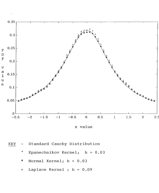
(5.2)

r = 1. 320. To illustrate the techniques reviewed in the chapter,

and to compare the three Kernels mentioned, given the difference in

their r values, the standard Cauchy density is estimated. Two

sample sizes are chosen,

(loa,

000 and 100 replications), these

representing a "large" and "small" sample respectively. The choice

of window width is determined using the technique of Tapia and

Thompson (1976). Figure 5.1 illustrates the results obtained for

100,000 replications, and given the asymptotic properties presented

in Section 3 it is expected that all of the estimated densities

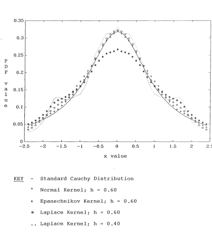
will be very similar. In Figure 5.2 when only 100 replications are

used, some differences, particularly with the Laplace Kernel, are

noticeable, suggesting that in small samples differences do exist

between different Kernels. However, these results are only

illustrative and the differences obtained with this example may not

FIGURE 5.1

Comparison of Different Kernels for Cauchy

Distribution Using 100,000 Replications

0.35

0.3 +

+ +

P 0.25 +

D

+

F

_0.2

+

v

a

1 0.15

u

e

it

0.1

0.05

0

-2.5 -2 -1.5 -1 -0.5 0 0.5 1 1.5 2 2.5

x

value

KEY

Standard Cauchy Distribution

o

Epanechnikov Kernel; h

=

0.03

*

Normal Kernel; h

0.03

P

D F

v a

1 u

e

FIGURE 5.2

Comparison of Different Kernels for Cauchy

Distribution Using 100 Replications

0.35~----~---.---~----~---.---~----~---.---.---,

0.3

0.25

0.2

0.15

0.1

0.05

*'

0* _d7

*'

~'

y~** +0 o .

*'

+ 0'* +ip,*

0+ _o

o~----~----~~----~----~---~----~---~----~---~----~

-2.5 -2 -1.5 -1 -0.5

o

0.5 1 1.5 2

x

value

KEY

Standard Cauchy Distribution

o

Normal