Test bed and sensor platform for building usage profiling

(1)

MASTER THESIS :

Test Bed and Sensor Platform

for Building Usage Proling

Peng Liu

Supervisors :

Peter Fuhrmann - PHILIPS Research Europe Karin Klabunde - PHILIPS Research Europe Nirvana Meratnia - University of TWENTE

Company :

PHILIPS Research Euroupe

Training Period :

(2)

(3)

Preface

The project is working towards a methodology and a tool framework that enable the accurate performance prediction of energy saving measures prior to a building retrot project. The attainable savings by advanced lighting and building control solutions heavily depends on the behavior of occupants and how other building specic conditions. A wireless sensor monitoring system is therefore introduced to audit and assess space utilization, occupancy and light conditions.

Daylight used to be the primary light source before the world rst long-lasting, practical electric light bulb invented by Tomas Edison in 1879. Although modern lighting technology allows us to provide sucient light intensity under almost any circumstance, daylight is still primary choice for internal illumination, not only for energy saving but also for a healthy working environment.

In this master thesis project, internal daylight intensity will be measured by wireless sensor network for a relatively short term in a representative part of the building. Relation between internal and external daylight radiation will be concluded from the collected data. Eventually this relation will be applied in concluding annual internal daylight intensity according to long-term external daylight records.

(4)

Acknowledgments

I would like to thank Peter Fuhrmann and Karin Klabunde, my supervisors at Philips Research Europe, who oered me this wonderful opportunity. Thank you for your encour-agement, support and guidance. I would also like to thank my supervisor in University of Twente, Nirvana Meratnia, thank you for your monthly advice and feedback. Without you this thesis would not have been possible.

I would like to thank my colleagues and friends, thank you for your support and making my life lled with fun and joy.

At last I would like to thank my parents, thanks for always supporting me and believing in me.

Thank you!

(5)

iii

Summary

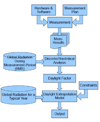
In this thesis, a complete procedure of internal daylight auditing with wireless sensor network was introduced. There are three stages involved:

In the measurement stage, internal daylight intensity is measured by wireless sensor network for 4 to 6 weeks. In the analysis stage, a methodology was introduced to conclude internal daylight intensity from outside global radiation, based on the data collected in measurement stage. In the simulation and extrapolation stage, internal daylight availability for a complete year was determined.

With the methodology introduced in this thesis, annual internal daylight intensity can be concluded from short-term measurement results collected by wireless sensor network and long-term global radiation records.

(6)

(7)

Nomenclature and Terminology

din Internal daylight intensity which is the daylight intensity inside proposed building, measured by wireless sensor network by the unit lx. Also referred as internal daylight availability;

DF Daylight factor, which is used to describe the relation between internal and external daylight intensity. Equals to the ratio of the internal daylight intensity to the external daylight intensity;

DFmean Average daylight factor which used to describe the relation between external and internal daylight radiation in overcast day;

GR Global solar radiation, including direct and diuse components of solar radiation model;

N Cloudiness value describes the quantity of cloud by the unit okta;

N R Node result measured by node (by the unit mV);

p(DF) Probability density function of daylight factor;

P P M CC, denoted byr Abbreviation for Pearson Product-Moment Correlation Coecient. PPMCC is A measure of linear dependency between two variables. The value is between -1 and +1 inclusively. Positive value indicates that one variable increasing is accompanied by increasing of the other value, otherwise, negative value indicates decreasing.

RD Direct component of daylight (also referred as direct daylight, sunlight or direct solar radiation);

Rd Diuse component of daylight (also referred as diuse daylight, skylight or diuse solar radiation);

BMS Abbreviation for Building Management System. Common BMS is a computer based control system installed in buildings monitors the buildings mechanical and electrical equipments, including ventilation, lighting and power system. In this case, BMS indicates the building management system which is applied in Building 34, High Tech Campus, monitoring articial light status, power consumption and global radiation on top of the building;

Light Zone: Zones in which daylight has same behavior;

Measurement Duration: Time duration between measurement starts and measurement ends; Measurement Period: Time interval between two measurement samples on same

measure-ment point;

Node Result Conversion Formula: Formula which used to convert node result (mV) into day-light intensity (lx);

(8)

Okta: Unit of measurement to describe the amount of cloud cover at a given location on the ground. The value ranges from 0, which means completely clear, to 8, which means completely overcast. Value 9 is used to describe the situation in which sky is not able to be observed, because of some extreme weather conditions like heavy snow or dense fog;

Scenario: Scenario is dened by the combination of variables which impact daylight measure-ment, including room orientation, occupation, cloudiness, etc;

Section: Part of a building (on the same oor);

(9)

List of Figures

2.1 Workow of Combined Project . . . 4

3.1 Solar Radiation Spectrum . . . 11

3.2 CIE Standard Human Eye Spectral Sensitivity . . . 12

4.1 Floorplan . . . 15

4.2 Light Zones . . . 17

4.3 Node Deployment in Room 1.044 . . . 18

4.4 Node Deployment in Room 1.043 and 1.045 . . . 19

4.5 Node Deployment in Room 1.037 and 1.039 . . . 19

4.6 Measurement Point 5 and 6 . . . 20

4.7 Measurement Point 3 and 4 . . . 21

4.8 Measurement Point 21 . . . 22

5.1 Internal and External Daylight Intensity in Overcast Holiday, North Room . . 27

5.2 Internal and External Daylight Intensity in Overcast Holiday, South Room . . 28

5.3 PPMCCs in Room 1.037 in Two Weeks . . . 30

5.4 PPMCCs in Room 1.044 with Dierent Cloudiness . . . 31

5.5 PPMCCs in Room 1.037 with Dierent Cloudiness . . . 32

6.1 Daylight Factor Calculation Flow . . . 40

6.2 PDF of Daylight Factor on Desk in Light Zone 2, Clear Working Days . . . . 41

6.3 PDF of Daylight Factor on Desk in Light Zone 1, Partly Cloudy Holiday . . . 42

6.4 PDF of Daylight Factor on Desk in Room 1.045, Partly Cloudy, Working Days 43 7.1 Internal Daylight Simulation Algorithm with BMS Records . . . 46

7.2 Accumulative Daylight Hours per Day . . . 47

7.3 Internal Daylight Simulation Algorithm with 10 Years Records . . . 48

7.4 Accumulative Daylight Hours per Day on Desk, Measurement Point 7 . . . . 49

7.7 Hourly Daylight Intensity on Inner West Desk, Room 1.044 . . . 51

8.1 Light Zones . . . 54

8.2 Estimated Minimum Measurement Period (CI = 90%, Relative Sampling Error = 5%) . . . 55

A.1 CM5000 Wireless Sensor Node . . . 58

A.2 Modify and Send Request in BMF . . . 58

A.3 KNMI Weather Station 370 (Green Arrow) and High Tech Campus 34 (Marker A) . . . 59

B.1 EXTECH HD450 . . . 61

B.2 Value Convert Formulae Comparison . . . 62

(12)

C.1 Estimated Minimum Measurement Period

(CI = 90%, Relative Sampling Error = 10%) . . . 64

(13)

List of Tables

5.1 PPMCCs between Internal and External Daylight Intensity in Overcast Holiday 29

5.2 PPMCCs between Nodes . . . 34

5.3 PPMCCs between Nodes . . . 34

6.1 Linear Regression between Internal and External Daylight Intensity in Overcast Holiday . . . 36

6.2 Sky Type and Cloudiness . . . 39

6.3 Estimated Parameters for Three Measurement Points . . . 44

D.1 Parameter Estimation Results, Room 1.044, 1.037 and 1.039 . . . 65

D.2 Parameter Estimation Results, Room 1.045 and 1.043 . . . 66

(14)

(15)

Chapter 1

Introduction

This master thesis, combined with previous internship, is related to the EnPROVE project [5], whose main objective is to provide recommendation for building renovations regarding energy saving. In oces, one of the major attainable energy saving sources is articial lighting. In this internship and master thesis combined project, daylight monitoring system and corresponding software will be deployed and congured to measure daylight intensity in a section of a real building for a relatively short period, to assess daylight availability inside this building.

The system which is used to accomplish this work should be able to measure and deliver the daylight availability (lux) and store the results to local les with relevant information. A wireless sensor monitoring system is therefore introduced. Wireless sensor nodes are small in size, which make them easy to be deployed. With these nodes, daylight availability can be measured on more ne-grained level. For example the measurement can be done simultane-ously on every desk in a room.

In previous work [41], a complete methodology of deploying, conguring wireless sensor monitoring system, and converting node results to daylight intensity has been created. On wireless sensor network side, several nodes with light sensors will be deployed at selected po-sitions. When running the infrastructure, a PC is used to run a program that collects results, modies nodes tasks, and saves results on the control side. The program running on the nodes should be easy to modify from the control side. Current hardware vendors design and produce their products abiding some public standards. This oers an easy way for developers to create simple functions in accordance with these standards. With these prerequisites, we choose a combination of hardware, standards and operating system to achieve our goals.

The node type we choose is CM5000 [4] produced by Advantics [1] which is compliant to TelosB standard. The operating system we choose is TinyOS [11], which is an open source, event-triggered system and designed for low-power wireless devices.

In this thesis, a methodology of concluding the relation between internal and external daylight availability will be introduced, and recommendations about applying wireless sensor network in daylight assessment and auditing will be given according to measurement result analysis. Finally, the methodology will be applied to conclude internal daylight availability for a typical or proposed year.

In Chapter 2, workow of the entire project will be introduced, from data collection to model creation and investigation issues for every stage in the workow. In Chapter 3, related work will be introduced as well as terms explanation. The content of Chapter 4 is about

(16)

(17)

Chapter 2

Research Topics

For a long time, daylight is the primary attainable light source for human beings. Even nowadays, as modern engineering allows us to provide adequate light intensity under almost any circumstances, daylight is still crucial for internal space, not only for energy saving, but also for a healthy working environment.

In this chapter, an overview of this project will be introduced. Research topics will be described for each stage of workow.

2.1 Workow

Workow of this combined project is illustrated in Figure 2.1:

This workow consists of 3 stages: measurement, analysis and extrapolation.

In the rst stage, wireless sensor nodes will be congured and deployed to measure daylight, according to measurement plan. The criteria of making this measurement plan are trying to cover every possible situation, and collect enough data to support our further data analysis.

After collecting all measurement results, node results will be extracted from raw data. Since the measurement is conducted during holidays as well during normal working days, node results consist of daylight contribution and articial light contribution when articial light is on. To conclude the relation of internal and external daylight, articial light contribution will be removed. Before analysis, node results, which are measured by the unit of millivolt, will be converted to internal daylight intensity, by the unit of lx.

In the second stage, the relation between internal and external daylight will be concluded. A typical concept is daylight factor (DF), which is the ratio of internal daylight intensity to external global radiation:

DF = din

GR

(2.1)

(18)

[image:18.595.97.491.163.644.2]

(19)

2.2. Research Topics 5

Normally the daylight factor will be used to calculate internal daylight intensity for overcast days. When it is clear outside, glare and reection will strongly impact this value. In following chapters, dierent variables impact, like cloudiness and occupancy, will be evaluated, and daylight factor will be concluded in typical form and probability distribution function.

In the third stage, daylight factor will be applied to build up a model. The objective of this model is to extrapolate the possible daylight intensity on a specic measurement point. Details about this model will be elaborated in Chapter 7.

2.2 Research Topics

For the measurement stage, researches focus on details of hardware and software, including how to deploy the wireless sensor network and congure the software, and details about measurement plan, including optimal measurement period and position, etc. The topics about hardware and software have been done in previous work. In Appendix A there is a brief introduction. The measurement plan will be introduced in Chapter 4. After analysis stage, the recommended measurement plan will be given, in Chapter 8.

For the analysis stage, researches focus on several topics. First, variables which impact internal daylight measurement and their aect will be evaluated. If a variable will impact the indoor daylight factor greatly, measurement results will be categorized and analyzed according to the value of this variable. Second, the method of analysis should be reliable. This is also the cornerstone of the entire project. At last, the required database should be listed, minimum requirement of input data will be concluded as a recommendation for daylight extrapolation.

(20)

(21)

Chapter 3

Related Work

Daylight is a phenomenon appears every day and closely related to our life. People did their research on daylight from long time ago. A variety of methods provides the developers a lot of alternatives, on the other hands a large amount of work are required to evaluate those methods.

In this chapter, related work will be introduced according to several investigation topics about daylight behavior and measurement, including:

• Measure internal daylight intensity;

• Measure/estimate external daylight intensity;

• Conclude relation between internal and external intensity;

• Conclude internal daylight distribution;

• Estimate minimum measurement duration before the measurement.

3.1 Related Work

In this project, internal daylight intensity will be measured by wireless sensor network. Wireless sensor node deployed in this project is CM5000 produced by Advantics [1]. In previous project [41], an introduction about running the wireless sensor monitoring system and converting light intensity measured by nodes (in the unit of mV) into light intensity (in the unit of lx) was provided. According to these work, daylight can be measured and converted into light intensity accurately. Details about wireless sensor monitoring system and value conversion method will be introduced in Appendix A and Appendix B.

External daylight intensity can be measured or calculated. Hourly external daylight in-tensity recorded by professional weather station of KNMI [8] for several decades is available. On the other hand, Building Management System (BMS) in HTC 34 records minutely global radiation for the last one year (from June, 2011 to July, 2012).

Studies about daylight models which are used to estimate daylight intensity started from decades ago [49] [16]. Some comparison work has been done to evaluate dierent models [64]. Daylight models are usually created not only for estimating daylight intensity but further purposes. Most of the daylight models are created to help designing a solar energy system for a location lacking of data base.

(22)

Mathematical models which describe daylight behavior can be categorized as spatial models and temporal models. Spatial models are created intending to describe the relation between internal and external daylight intensity of a building or the daylight distribution inside a building. Temporal models are created intending to estimate external daylight intensity the proposed location.

There are some other models which are developed to investigate other related issues about daylight. Decomposition models are created to decompose global radiation into direct and diuse components. These models are widely used in solar energy system design. Cloudiness models are created to calculate the impact of cloudiness to the solar radiation. Spectral models are developed to describe the relation between light spectrum and visibility. In this report, only daylight spectral models will be discussed.

Besides the mathematical models, almost all of these issues related to daylight can be concluded from measurement results. For example, if we want to know the relation between daylight intensity on a desk inside a building and on the roof of the building, we can just measure for a period of time and conclude the relation from measurement results.

3.1.1 Spatial Model

To conclude the relation between internal and external daylight intensity, spatial daylight models will be applied. There are three types of spatial models. Factor models are created based on the concept of daylight factor, which is the ratio of indoor daylight radiation on proposed surface to external daylight intensity on a horizontal surface. This factor is also called daylight factor. Ray tracing models intend to calculate and estimate the daylight intensity after every reection. These models are accurate and usually used for simulation of internal daylight behavior, like simulating and illustrating the results of architectural design. On the other hand, the high complexity requires higher calculation time than other models. The basic idea of radiosity models is regarding the window as a light source. The radiation of the window can be calculated according to solar altitude, solar azimuth, global radiation and size of the window. According to the law of conservation and the fact that light intensity reected to the outside through the window is far less than the incoming, the radiation is regarded as completely absorbed by the internal surfaces like walls, ceiling, work planes and oor. Then radiation can be estimated from the energy distributed in the room.

(23)

3.1. Related Work 9

[39] [25]. In this thesis, it will be extended to every type of sky with the methodology we introduced.

Similar as external daylight intensity, internal daylight distribution can also be measured or calculated. In some researches, a model of proposed room is applied to simulate daylight distribution in a real room. Some organizations and standards also provide us complete mathematical tools for computing visualizing internal daylight distribution [61] [7] [21] [27] [18] [59] [52].

3.1.2 Temporal Model

Spatial models are time-invariant models. Time will not be considered in those models. In temporal models, time will be introduced as the crucial independent variable and the relation between time and global radiation will be concluded.

Temporal daylight model has been studied for many years. Early models like Moon model [49] created in 1940s are still used in modern engineering.

Reading all the documents to learn every detail about these temporal daylight models is inecient and unnecessary. Instead, comparison researches have been done, by briey intro-ducing, comparing the formulae, constants, variables in the models, and also by comparing models performances with real data. To learn the models created before 1980s, RICHARD E. BIRD and ROLAND L. HULSTROM works, published in 1981 [17], briey introduced and compared 7 models, including ATWATER AND BALL MODEL [13], DAVIS AND HAY MODEL [23], WATT MODEL [63], HOYT MODEL [24], LACIS AND HANSEN MODEL [33], BIRD MODEL [15] AND SOLTRAN MODEL [16]. In their previous work published in 1980 [16], another several models, MACHTA MODEL [44], ASHRAE MODEL [45] [29] and MAJUMDAR MODEL [46], were introduced, but not compared. All of these models are created in 1970s. These models also focus on dierent aspects of solar radiation propagation, like atmospheric extinction [33], direct solar radiation [46], etc. What is noteworthy is that some of these models keep improving in the last several decades, like ASHRAE MODEL, which updates basically every 2 years. For models created after 1980s, there are also works which evaluate those models. Like L. T. WONG and W. K. CHOW's work published in 2004 [64], which compared several commonly used models, including IQBAL MODEL [26] and ASHRAE MODEL [12]. Decomposition models were also introduced and compared in this paper. In other researches [22], daylight models are compared with measured data.

In temporal models, formulae which consist of meteorological constants and variables are created to calculate the daylight intensity.

3.1.3 Cloudiness Model

(24)

Stephenson [31] and formula concluded by Kasten and Czeplak [30]. In the early year when Kimura and Stephenson did their research, the unit of okta, which is used to describe the cloudiness today, has not been invented. In their work we can see that cloudiness is described by experienced observers. Kasten and Czeplak work based on 10 years measurement in Hamburg. Their formula which can be used to describe the relation between global radiation and cloudiness are widely used today [57] [56].

Following equation is developed by Kasten and Czeplak that shows the relation between global radiation when cloudiness isN and the clear sky global radiation.

G(N)

G(0) = 1−0.75(

N

8) 3.4

(3.1)

G(0) can be calculated with the clear-sky model. With the measurement of okta value

N, global radiation can be calculated. According to another research, this equation needs parameter calibration when applied in another location. Quadratic formula also performed well in this step.

3.1.4 Decomposition Model

The purpose of decomposition models is to decompose the long-term measured global radiation into direct and diuse components. Most of the daylight models are created to help designing a solar energy system for a location lacking of data base.

There are also several common used decomposition models. Among them LIU and JOR-DAN model [40] is appreciated in this project, because it does not require atmospheric in-formation and this model is concluded according to the data from 98 localities in the USA and Canada from 19 ◦ _{to 55} ◦ _{N. There are several other commonly used models, including}

ORGILL AND HOLLANDS MODEL [50], ERBS et al. MODEL [20], SPENCER MODEL [58], REINDL et al MODEL [53], SKARTVEIT AND OLSETH MODEL [55], MAXWELL MODEL [14], VIGNOLA AND McDANIELS MODEL [62], LOUCHE et al. MODEL [42] and LAM AND LI MODEL [34]. Some of these models are modication or improvement of old models, others are new models based on measurement results collected in another region. Direct and diused components will be concluded from the ratio that ground global radiation to corresponding extraterrestrial radiation.

3.1.5 Spectral Model

(25)

3.1. Related Work 11

[image:25.595.135.478.180.440.2]

The surface temperature of the Sun is about 5500◦C, according to NASA measurement [9]. The spectrum of solar radiation is close to that of a black body with temperature of 5800 K. When the radiation reaches the top of the atmosphere of the Earth, the spectrum is close to that of a black body with temperature of 5250◦_C_{. Solar radiation spectrum is shown in}

Figure 3.1.

Figure 3.1: Solar Radiation Spectrum

Sun emits X-rays, ultra-violet, visible light, infrared and even radio waves. In this project, we only care about the visible light which wavelength ranging from 380 to 780nm. Solar radiation has dierent intensity at each wavelength within this range. On the other hand, human eye sensitivity also varies from the wavelength of incident light. In visual neuroscience, spectral sensitivity is used to describe the sensitivity of human eye to dierent wavelength of light. The most widely-used spectral sensitivity model is CIE [3] standard published in 2004 [2], as shown in Figure 3.2.

(26)

Figure 3.2: CIE Standard Human Eye Spectral Sensitivity

GRlx=LE×GRppua

(3.2)

GRlxindicates the global radiation by the unit oflx,GRppuaindicates the global radiation measured by power per unit area. LE indicates the luminous ecacy.

3.1.6 Measurement Duration

Long-term [19] [37] [38] and short-term experiments [28] are conducted in dierent cities. Studies about short time internal light behavior measurement are also available. At this moment, most of these experiments are conducted to conclude the internal articial light use and energy consumption. Results shows that short-term measurement during 2 weeks is already enough to draw some conclusions. To conclude the internal daylight availability, longer measurement duration is recommended in case of leading to unreliable conclusions.

3.2 Recommendations

(27)

3.2. Recommendations 13

building. Decomposition model usually created to decompose global radiation into direct and diuse daylight. Most of the popular daylight models were created decades ago, like Iqbal model is created in 1983 and ASHRAE in 1999. Outdated constants and data measured by the equipments at that time make the model unreliable today. On the other hand, inappropriate choice among the variety of methods calculating the meteorological values also may lead the whole calculation to intolerable deviations. When applying spatial models for some special situations, external reection will signicantly change internal daylight. To analyze these situations, not only direct daylight but also solar altitude and azimuth should be calculated or measured, and a function to describe the direct daylight contribution according to solar altitude and azimuth should be created at same time. All of these modeling procedures are quite likely to introduce a larger deviation.

(28)

(29)

Chapter 4

Measurement

In this chapter, the details about the measurement will be elaborated.

4.1 Measurement Specications

In this section, details of measurement plan will be introduced, from the oorplan, node deployment and measurement period.

4.1.1 Floorplan and Oces

The measurement is conducted on the rst oor of Building 34, High Tech Campus, Eind-hoven. Floorplan is shown in Figure 4.1. Golden arrows indicate the direct daylight.

Figure 4.1: Floorplan

Oces were chosen according to the issues which may impact the daylight distribution, like room geometry, number of occupancies, side of building (room orientation N/S), and the

(30)

curtains (automatic curtain or regular curtain). Oce selection covered every type of oces in this section, according to these issues.

Oces included (as outlined in Figure 4.1) and oce specications are:

• Room 1.045, one person oce, on the south side, with automatic curtains;

• Room 1.043, one person oce, on the south side, with automatic curtains;

• Room 1.039, three persons oce, on the south side, with regular curtains;

• Room 1.037, four persons oce, on the south side, with regular curtains;

• Room 1.044, lab, with ve regular occupancies, on the north side, with regular curtains,

but never set down.

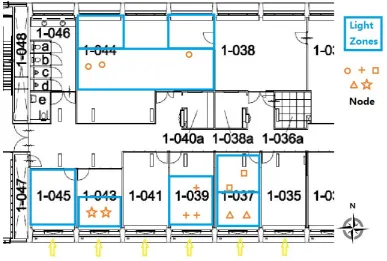
4.1.2 Light Zone

In this project, light zone indicates a zone in which daylight has same behavior. According to this concept, the total measurement area will be divided into smaller light zones. Mea-surement points can be chosen according to light zone, and the optimal measure point can be concluded.

As an investigation topic, light zone division rules will be concluded as recommendation in Chapter 8. Before this measurement, light zone will be divided according to oce geometry. As shown in Figure 4.2. For relatively small room in this section, the whole oce will be regarded as one light zone rst. After the measurement, the measurement division will be rened according to the measurement results. The measurement will be conducted in west and east part of room 1.044, which is bigger than the others. Room 1.044 will be divided into 2 light zones under this circumstance.

Details about the layout of each light zones and node deployment will be introduced in next section.

4.1.3 Node Deployment

One of the advantages of wireless sensor node is its small size. This allows us to deploy it on any point in the room. The proposed measurement points in this project are:

• On the desk. This is the direct way to measure daylight availability on each desk. But

in weekdays, node results will be impacted by occupancy;

• On the ceiling and measure the reection (sensor downwards). In previous tests, some

(31)

4.1. Measurement Specications 17

(32)

• Near the window. The advantage of measuring near the window is that the node results

will hardly be impacted by occupancy or curtains. On the other hand, the measurement scale of sensor on the node is only about 2,000 lx. If the light intensity incident on the sensor is higher than this value, the sensor will work in the non-linear section, which means the result is not reliable. Light intensity near the window exceeds this limit more frequently than light intensity inside the room, even in an overcast winter day in which solar radiation on the ground is almost the weakest in a year;

• On the ceiling and measure the articial light intensity (sensor upwards, towards the

articial light). These nodes will not deliver us meaningful light intensity to conclude the daylight factor. These results will be used to conclude the articial light state is on or o.

According to these rules, node deployment in every light zone is shown below, from Figure 4.3 to 4.5:

Figure 4.3: Node Deployment in Room 1.044

What is noteworthy is, in room 1.039, three nodes are deployed at same point near the window. The dierences are the directions their sensors towards. The dierences between these three nodes results can also help us to dene the optimal measurement points.

(33)

Figure 4.4: Node Deployment in Room 1.043 and 1.045

(34)

(35)

(36)

(37)

4.2. Raw Data Process 23

4.1.4 Measurement Duration and Period

In some researches, measurement duration of short-term daylight measurement is dened as 2 weeks. In this project, recommended measurement duration will also be concluded in analysis stage. When starting this measurement, considering the capability of wireless sensor network and the corresponding software, the measurement duration is dened as 4 to 6 weeks, and measurement period as 6 minutes.

4.2 Raw Data Process

The internal daylight intensity will be delivered as node results by the wireless sensor nodes by the unit milli-volt, together with the articial light intensity. To conclude the relation between internal and external daylight intensity, articial light component will be removed, and daylight component will be converted in light intensity by the unit lx.

Remove Articial Light Component

To remove the articial light component from measurement results, we need to know:

• Articial lights contribution, which is the articial light intensity on every measurement

points;

• Articial light status, in this project, articial lights in the same room was controlled

by one non-dimmable switch, which means articial light is either on or o.

In Building 34, High Tech Campus, building management system (BMS) will record the oces articial lights status, but not for laboratories. The articial light status in room 1.043, 1.045, 1.037 and 1.039 can be extracted from BMS measurement logs. As mentioned in previous section, to conclude the articial light status, a special node was attached on the ceiling and its sensor towards the articial light. Articial light status in room 1.044 will be concluded from this node result [25].

To conclude the articial light component, there are three major ways:

• Find a special situation, articial light is on when there is no occupant and it is dark

outside. Articial light component can be directly read from the measurement. This method is very ecient when it is winter, during which time it is getting dark very early;

• Compare two adjacent samples between which articial light is switched;

4.2.1 Value Conversion

(38)

(39)

Chapter 5

Scenario-Dependency and Internal

Daylight Distribution

In this chapter, three topics will be elaborated. In Section 5.1, daylight factor will be introduced. Variables which impact internal daylight availability will be investigated and evaluated in Section 5.2, 5.3 and 5.4. Internal daylight distribution will be discussed in Section 5.5.

Hypothesis for daylight analysis will be given in Section 5.6.

5.1 Daylight Factor

Daylight factor is the ratio of internal daylight intensity to external daylight intensity. Typically, daylight factor is used to describe the daylight availability in overcast days. Many studies and experiments show that in overcast day, daylight factor for a specic room is a constant value. Before investigating daylight factor, its concept should be specied for this project.

In this project, daylight factor in building 34, High Tech Campus, is dened as:

DF = din

GR

(5.1)

DF indicates daylight factor, din indicates internal daylight intensity, and GR indicates global radiation measured by BMS.

As a common sense, if someone is sitting in front of a desk, daylight availability on the desk will be altered. Typical daylight factor theory just investigated the daylight factor in overcast days. But when investigating daylight availability for a typical year or a specic period of time, daylight factor for overcast day is not enough. In typical theories, room orientation and geometry is usually evaluated as the variables which impact daylight factor calculation. In this project, since daylight factor will be delivered as desk-specic values, the information of room orientation and geometry has been included implicitly. In this project, the variables which will be evaluated are occupancy and cloudiness.

(40)

To evaluate each variable eect, occupancy and cloudiness will be quantied rst. Room occupation can be regarded as a binary value, 1 indicates the room is occupied, and 0 indicates the room is empty. To quantify the cloudiness, the unit of okta will be introduced. In meteorology, okta is used to describe the cloud cover observed from the ground, with the value ranging from 0, which indicates completely clear, to 8, which indicates completely overcast.

Variables which impact daylight factor will be investigated and evaluated one by one. First daylight factor of overcast holiday will be investigated, which is also the typical daylight fac-tor. Then occupancy and cloudiness eects will be evaluated respectively. At last, hypothesis of daylight factor calculating will be given.

On the other hand, typical daylight factor theories attempt to calculate daylight factor in every corner of a room. Regarding daylight auditing or estimating energy saving potential, daylight factor on each desk is crucial. So eventually, daylight factor will be delivered as discrete values, on dierent desks.

5.2 Daylight Factor in Overcast Holiday

Take May 5th, Saturday, 2012 as an example. According to KNMI hourly records, the cloudiness is 8 okta all the day. Figure 5.1 shows the relation between BMS global radiation and daylight intensity in Room 1.044, Light Zone 1 (node deployment is shown in Figure 4.3):

Figure 5.2 shows the internal and external daylight intensity in Room 1.037 (node deploy-ment is shown in Figure 4.5):

In Figure 5.1 and 5.2, we can see that the linear dependency between internal and external daylight intensity is very strong. To describe this relation, Pearson product-moment corre-lation coecients (referred as PPMCCs afterwards) were calculated. As shown in Table 5.1 (light zone division and node deployment are shown in Figure 4.3, 4.4 and 4.5):

In statistics, if PPMCC is larger than 0.8, relation between two variables can be regarded as linear. Data in Table 5.1 indicate that relation between internal and external daylight intensity is linear, which means we can use a function in the form of:

din=β0+β1×GR

(5.2)

(41)

5.2. Daylight Factor in Overcast Holiday 27

(42)

(43)

5.2. Daylight Factor in Overcast Holiday 29

Table 5.1: PPMCCs between Internal and External Daylight Intensity in Overcast Holiday

Date: May 5th, 2012

Light Zone Room Orientation Measurement Point PPMCCs Room 1.044, Light Zone 1 North On the desk 0.9639 Room 1.044, Light Zone 1 North On the ceiling 0.9661 Room 1.044, Light Zone 1 North Near the window 0.9956 Room 1.044, Light Zone 2 North On inner desk 0.9698 Room 1.044, Light Zone 2 North On outer desk 0.9615 Room 1.044, Light Zone 2 North On the ceiling 0.9758 Room 1.044, Light Zone 2 North Near the window 0.9958 Room 1.037 South On inner, east desk 0.9842 Room 1.037 South On inner, west desk 0.9837 Room 1.037 South On outer, west desk 0.9682 Room 1.037 South On outer, east desk 0.9798 Room 1.037 South Near the window 0.9795

Room 1.037 South On the ceiling 0.9811

Room 1.039 South On inner desk 0.9769

Room 1.039 South On outer, east desk 0.9547 Room 1.039 South On outer, west desk 0.9624

Room 1.039 South Window, up 0.9804

Room 1.039 South Window, in 0.9855

Room 1.039 South Window, out 0.9786

Room 1.045 South Near the window 0.9824

(44)

5.3 Occupancy Eect

PPMCCs between three measurement points in Room 1.037 and global radiation are shown in Figure 5.3. This room is regularly occupied by interns. As we can see, during weekends or public holiday (May 18th), PPMCC is relatively higher than normal working days. Results also show that for some days, PPMCCs is lower than 0.8, indicating that the points are far from lying on a straight line.

Figure 5.3: PPMCCs in Room 1.037 in Two Weeks

5.4 Cloudiness Eect

(45)

5.4. Cloudiness Eect 31

(46)

(47)

5.5. Internal Daylight Distribution 33

5.5 Internal Daylight Distribution

The study of internal daylight distribution intends to provide a global view of daylight availability in the section of proposed building [48] [35]. With this information, the relation between measurement points can be concluded, and the possibility to minimize and optimize daylight measurement points can be investigated.

Some researches provide mathematical models to calculate daylight distribution in rooms. In this project, relation between measurement points will be concluded according to measured data and some recommendations will be given.

There are three possible relations between 2 measurement points:

• 1, Measurement results on 2 proposed points are basically the same;

• 2, Measurement results on 2 proposed points have strong linear dependency, but the

contributions of daylight are dierent;

• 3, There is no obvious relationship between measurement results on 2 proposed points.

For the rst two cases, daylight on one measurement point can be concluded from the measurement results on the other point. If one measurement point has no obvious relationship with any other node, then this measurement point can be regarded as necessary.

To achieve the goal, PPMCCs between nodes which indicate the linear dependency between every two measurement points will be calculated.

With Matlab, PPMCCs between every pair of nodes will be calculated. Table 5.2 shows all the pairs between which PPMCCs is higher than 0.9, which means strong linear dependency.

As mentioned before, only a small part of measurement results near the window is avail-able because of the limit of the sensors. Tavail-able 5.3 shows the node pairs with strong linear dependency and not measuring near the windows.

Recommendations of optimal and minimal measurement points will be given in Chapter 8.

5.6 Hypothesis for Daylight Factor Analysis

(48)

Table 5.2: PPMCCs between Nodes

Node A Node B PPMCCs

Room 1.044, Inner Desk, West Room 1.044, Window, Upward 0.9299 Room 1.044, Inner Desk, West Room 1.044,Ceiling, Downward 0.96674 Room 1.044, Window, Upward Room 1.044,Ceiling, Downward 0.91912 Room 1.044, Window, Upward Room 1.044, Window, Upward 0.99288 Room 1.044, Window, Upward Room 1.044, Outer Desk, East 0.95131 Room 1.044, Window, Upward Room 1.039, Window, Upward 0.92072 Room 1.044, Window, Upward Room 1.039, Window, Out 0.94157 Room 1.044,Ceiling, Downward Room 1.044, Window, Upward 0.90196 Room 1.044, Window, Upward Room 1.044, Outer Desk, East 0.95237 Room 1.044, Window, Upward Room 1.039, Window, Upward 0.91126 Room 1.044, Window, Upward Room 1.039, Window, Out 0.93996 Room 1.044, Inner Desk, East Room 1.044, Ceiling, Downward 0.93445 Room 1.039, Inner Desk, East Room 1.039, Outer Desk, East 0.92549 Room 1.039, Inner Desk, East Room 1.039, Outer Desk, West 0.91841 Room 1.039, Outer Desk, East Room 1.039, Outer Desk, West 0.94736 Room 1.039, Window, Upward Room 1.039, Window, Out 0.97458 Room 1.039, Window, Upward Room 1.037, Window, Upward 0.9109 Room 1.037, Inner Desk, West Room 1.037, Ceiling, Downward 0.91818 Room 1.037, Outer Desk, West Room 1.037, Outer Desk, East 0.98101 Room 1.037, Outer Desk, West Room 1.037, Window, Upward 0.91553 Room 1.037, Outer Desk, East Room 1.037, Window, Upward 0.94549 Room 1.043, Outer Desk, West Room 1.043, Outer Desk, East 0.998

Table 5.3: PPMCCs between Nodes

Node A Node B PPMCCs

(49)

Chapter 6

Daylight Factor

According to previous chapter, daylight factor depends on cloudiness, occupancy and room specications. In this chapter, typical daylight factor will be concluded with regression anal-ysis and for complex situations (with occupancy and under clear sky) daylight factor will be delivered as probability density function.

6.1 Overcast Sky, without Occupancy Daylight Factor

According to Table 5.1, there is strong linear dependency between internal and external daylight intensity during overcast holidays. The relation between internal daylight and ex-ternal global radiation can be described as:

din=β0+β1×GR

(6.1)

under this circumstance. β0 indicates internal daylight when external global radiation is

0, which is 0lxtheoretically. β1 is daylight factor.

To conclude daylight factor under overcast sky, linear regression will be applied.

Linear regression is an approach which intends to model the linear dependency between dependent variables and independent variables. In this case, the objectives are β0 and β1.

Matlab provides a complete solution of linear regression. In this stage, β0 and β1 were

concluded by the function regress in statistics toolbox. Results shown in Table 6.1:

6.2 Statistical Daylight Factor

Since daylight factor is room-, occupancy- and cloudiness-dependent value, we need to conclude daylight factor for the other scenarios and try to cover all of them. For a clear or partly cloudy day, if applying regression analysis to other scenarios, multivariate regression is required, because internal daylight depends on several dierent variables under these circum-stances. An available model [43] is to decompose daylight as direct and diuse components and conclude multivariate linear regression:

(50)

Table 6.1: Linear Regression between Internal and External Daylight Intensity in Overcast Holiday

Light Zone Measurement Point β0 β1

Room 1.044, Light Zone 1 On the desk 47.2393 0.041011 Room 1.044, Light Zone 1 On the ceiling 31.9025 0.018658 Room 1.044, Light Zone 1 Near the window 39.7479 0.46782 Room 1.044, Light Zone 2 On inner desk 42.3276 0.026763 Room 1.044, Light Zone 2 On outer desk 37.1523 0.17083 Room 1.044, Light Zone 2 On the ceiling 31.7846 0.022684 Room 1.044, Light Zone 2 Near the window 47.04 0.43025 Room 1.037 On inner, east desk 21.8566 0.051993 Room 1.037 On inner, west desk 25.4268 0.05463 Room 1.037 On outer, west desk 48.9793 0.14135 Room 1.037 On outer, east desk 31.3468 0.16379 Room 1.037 Near the window 66.2285 0.24048 Room 1.037 On the ceiling 21.2983 0.019442 Room 1.039 On inner desk 22.1697 0.021817 Room 1.039 On outer, east desk 49.5216 0.098091 Room 1.039 On outer, west desk 23.5815 0.08897 Room 1.039 Window, up 79.8 0.23459 Room 1.039 Window, in 23.7859 0.033812 Room 1.039 Window, out 64.5477 0.26178 Room 1.045 Near the window 57.472 0.28277

(51)

6.2. Statistical Daylight Factor 37

din=β0+β1×Rd+β2×RD

(6.2)

Rdindicates the diuse component andRD indicates the direct component of global radia-tion. To calculate these two components, several daylight decomposition models are available. Results show that this approach is not satisfying. The possible reasons are:

• Some decomposition models require detailed information about atmosphere, which is

hard to estimate or requires professional equipment to measure. These parameters are quite location-dependent, previous studies just oer us a possible but not reliable solution;

• Some decomposition models require the estimation of extraterrestrial solar radiation.

Same as the others, these models also intended to provide us a possible but not reliable solution. Our objective is to estimate daylight availability as accurate as possible; any estimation deviation should be avoided;

• For some special situations, external reection will signicantly change internal

day-light. To analyze these situations, not only direct daylight but also solar altitude and azimuth should be calculated or measured, and a function to describe the direct day-light contribution according to solar altitude and azimuth should be created at same time. All of these modeling procedures are quite likely to introduce a larger deviation.

These disadvantages and problems are relatively dicult to settle or improve. It either re-quires professional meteorological equipments, dedicated run-time measurement, more com-plex mathematical models, or all of them.

On the other hand, the internal daylight measurement can be abstracted as a system working under dierent independent states. States are dened by the combination of room, occupancy and cloudiness information and also called scenario in this project. After the measurement and collecting cloudiness, occupancy information, we know the state in which the system is working for each sample. Since these samples are collected in dierent days, this measurement can be regarded as a test of repeated random sampling. Monte Carlo Method can be applied under this circumstance. If we categorize all the samples and conclude the probability density function for each possible value, this probability density function can be used to describe the daylight factor for complex situations.

6.2.1 Monte Carlo Method

(52)

A typical workow of Monte Carlo Method is:

• 1, Dene a domain of possible inputs;

• 2, Generate random input according to a probability distribution over the input

do-main;

• 3, Perform a deterministic computation on the inputs;

• 4, Aggregate the results.

Usually the inputs for Monte Carlo Method are randomly generated by computer according to a predetermined probability distribution. In this project, the random inputs are collected by nodes and BMS. In the third step, the corresponding computation is the same as the computation of typical daylight factor:

DF = din

GR

(6.3)

for every sample. The objective is to conclude the distribution ofDF in dierent scenarios, two conditions must be met:

• 1, Measurement must be repeated random sampling;

• 2, There must be sucient number of samples to lead to the distribution function

convergence.

As mentioned before, samples measured in the same scenario can be regarded as random sampling. For the second condition, the total number of samples for every measurement point is

10×24×7×6 = 10080samples

(6.4)

during 6 measurement weeks. In May and June, daylight time is longer than 12 hours every day. That ensures that there will be more than 5000 samples available for every measurement point, which is enough to conclude reliable results.

(53)

6.2.2 Sky Type

One requirement of Monte Carlo Algorithm is sucient number of samples. At Eindhoven, completely overcast sky and clear sky are quite normal, but not partly cloudy sky. If all the samples are categorized by every 1 okta, it is hard to gather adequate samples under 3, 4 or 5 okta during a short period of measurement time. A compromise solution is to analyze daylight factor under 3 dierent types of sky, as shown in Table 6.2:

Table 6.2: Sky Type and Cloudiness

Sky Type Cloudiness (okta) Clear =<2

Partly Cloudy 3 to 6

Overcast >= 7

6.2.3 Daylight Factor Calculation Algorithm

In summary, daylight factor calculation ow is shown in Figure 6.1:

First, node results will be extracted from the raw les. With the methods mentioned in previous chapters, articial light contribution will be removed, and node results will be converted to corresponding light intensity. After the renement, repeated samples will be removed, as well as the samples which were collected when it is completely dark outside. Then these rened data will be categorized according to measurement points, occupancy and cloudiness information, which is also called scenario in this report. In the next stage, parameters will be estimated. This work can be done with the functions oered by Matlab statistics toolbox. The nal conclusion will be a set of probability density function (PDF) of daylight factor distribution, which indicates the possible daylight factors in dierent scenarios as well as the probability of each possible value of daylight factors.

6.2.4 Parameter Estimation

Normal distribution is also known as Gaussian distribution. The probability density func-tion is:

f(x;µ, σ2) = 1

σ√2πe

−1 2(

x−µ σ )

2

(6.5)

(54)

(55)

In Room 1.044, curtains were never changed. All the samples can be regarded as measured under same circumstance. Parameters estimation results for clear working days and partly cloudy holidays are shown in Figure 6.2 and 6.3:

Figure 6.2: PDF of Daylight Factor on Desk in Light Zone 2, Clear Working Days

From these gures we can see, if we categorize the samples by cloudiness and occupancy, we can conclude corresponding normal distribution very well.

In Room 1.043 and 1.045, automatic curtains will be laid down to block the daylight when its intensity is too high for normal internal requirement. Daylight factors will be signicantly changed after the curtains were laid. Since automatic curtains only have two states, up or down, daylight factors will be investigated according to dierent states and two daylight factors will be concluded.

In Figure 6.4, daylight factor in Room 1.045 for working days under partly cloudy sky was shown. The yellow curve is the estimated normal distribution for daylight factors when cur-tains are not laid down. Average daylight factor is relatively higher under this circumstance. The blue curve shows the estimated normal distribution for daylight factors when curtains are laid down, which has a relatively lower average daylight factor.

(56)

(57)

(58)

σ for three measurement points which are on desks.

Table 6.3: Estimated Parameters for Three Measurement Points

Measurement Points Inner Desk, West Outer Desk, East Inner Desk, East

Occupancy Sky Type µ σ µ σ µ σ

No Overcast 0.046245 0.020212 0.13778 0.082677 0.027701 0.01084 No Partly Cloudy 0.043927 0.021041 0.12992 0.087013 0.026516 0.011396 No Clear 0.038578 0.018487 0.11691 0.086823 0.024261 0.01119 Yes Overcast 0.056278 0.028281 0.16484 0.089622 0.030804 0.012425 Yes Partly Cloudy 0.054916 0.029837 0.15525 0.093481 0.029836 0.013537 Yes Clear 0.045414 0.026941 0.11926 0.092361 0.026191 0.014135

From the table, we can nd several issues:

1, During working days, internal daylight intensity has a higher volatility (higher ¦Ò) than holidays. It is reasonable because with a person working in front of the desk, the body movement will alter the intensity.

2, The daylight factors expectation is higher in working days than in holidays, which means daylight contribution on each desk is averagely higher in working days than in holidays. Normally if a person sits in front of a desk, part of the light will be blocked, which will lead to a lower daylight factor. The explanations for this contradiction are:

• In this project, to simplify the question, the occupancy information is dened according

to the date. On the other hand, the measurement period (May, 5th to Jun 17th) is almost the period with the longest daylight time during a year, usually with the daylight time more than 14 hours a day. If a desk is occupied for 8 hours, there are still 6 hours during which the desk is not occupied. Samples measured during this period of time should be considered as ½®holidays½ ;

• A day which is categorized as ½®working day½ does not indicate that the desk is

always occupied during the day. During working hours, people could also be away from their desk because of meetings or personal reasons;

• When a person is working in front of his desk, extra light sources are switched on and

contributing to the internal light intensity, especially the screens. The contribution of these components is complicated to model, and it is regarded also as daylight in this project.

(59)

Chapter 7

Daylight Extrapolation Model

In previous chapter, the relation between internal and external daylight intensity, daylight factor, has been concluded according to the measurement results collected during a relatively short period. In this chapter this relation will be applied to extrapolate daylight availability on desks we measured for a whole year.

In this chapter, Monte Carlo Method [54] will be applied again. As mentioned before, the typical workow of Monte Carlo Method is:

• 1, Dene a domain of possible inputs;

• 2, Generate random input according to a probability distribution over the input

do-main;

• 3, Perform a deterministic computation on the inputs;

• 4, Aggregate the results.

In the extrapolation stage, the input generated by computer is daylight factor (DF). The domain of possible inputs are from 0 to 1 (internal daylight intensity cannot be negative and normally it cannot be higher than 1). Daylight factors will be generated according to the normal distribution, which expectationµand standard deviationσ are dened by cloudiness value (by the unit okta) and occupancy, according to the estimation results shown in previous chapter. The deterministic computation is:

ˆ

din=GR×DFˆ

(7.1)

ˆ

DF indicates the simulated daylight factor, which is the inputs generated in the second step. _dˆ_in _{indicates the simulated internal daylight. After the computation for large number}

of samples, conclusions can be draw from the simulation results.

There are two alternative sources of global radiation (GR). In HTC, 34, BMS minutely records for the last one year (Jun, 2011 to May, 2012) is available. On the other hand, dedicated global radiation records on the roof are not always available for a common building. In this case, global radiation recorded by KNMI weather station will be introduced.

(60)

7.1 Daylight Availability Extrapolation According to BMS

Re-sults

In HTC 34, BMS recorded the global radiation every minute. In this approach, internal daylight availability will be extrapolated following the workow shown in Figure 7.1:

Figure 7.1: Internal Daylight Simulation Algorithm with BMS Records

First, global radiation records and corresponding time stamps will be extracted from BMS raw data. Cloudiness value will be extracted from weather records according to the time stamp. Then daylight factors will be simulated and internal daylight intensity will be calcu-lated.

Simulated internal daylight intensity is available for every minute from Jun 2011 to May 2012 after this simulation procedure. To visualize the result, accumulative hours of daylight time per day in every month is shown in Figure 7.2 (take one desk in Room 1.044 as an example):

(61)

7.2. Daylight Availability Extrapolation According to 10 Years Records 47

Figure 7.2: Accumulative Daylight Hours per Day

and writing for more than 8 hours in May, June, July and August. Especially in July, daylight intensity is sucient for reading and writing for about 10 hours a day. In this month, it is highly recommended to make full use of the natural light during working hours for energy saving and healthy working environment.

This approach has two disadvantages. On the one hand BMS records are not available for all common buildings. On the other hand, records for a specic year are usually not typical. For example, usually the average daylight intensity is June is higher than that in May. From Figure 7.2, we can see that the average appropriate reading and writing time in May 2012 is longer than it in June 2011, because in this May there are more clear days in Eindhoven than usual.

7.2 Daylight Availability Extrapolation According to 10 Years

Records

To draw a typical conclusion, records in dierent years are required. In this project, 10 years (2001 to 2010) KNMI radiation records will be introduced as global radiation. The algorithm is shown in Figure 7.3:

(62)

(63)

What is noteworthy is that KNMI radiation records are in the unit of J/cm2. In this project, the records were translated to light intensity in the unit of lx by multiple the KNMI records with luminous ecacy, and luminous ecacy for 5800k blackbody radiation which value is93lm/W is applied.

Take Room 1.044 as an example, accumulative hours of daylight time per day in every month on three desks is shown in Figure 7.4, 7.5 and 7.6, corresponding measurement point is shown in Figure 4.3.

Figure 7.4: Accumulative Daylight Hours per Day on Desk, Measurement Point 7

On the other hand, internal daylight intensity can be extrapolated for every hour. Figure 7.7 is an example by showing hourly daylight on inner west desk in Room 1.044 in January and July.

For example, in July, averagely there is about 15 days in which daylight intensity at 12 o'clock (CET) is higher than1000lxon this desk. In January, averagely there is only 5 days in which daylight intensity at 12 o'clock is higher than 500lx. From this gure, we can see that in January, there is almost no potential to save energy by switching of articial light during working time, and in July, curtains or blinds are probably required to block the strong daylight around noon.

(64)

[image:64.595.74.470.107.360.2]

Figure 7.5: Accumulative Daylight Hours per Day on Desk, Measurement Point 6

[image:64.595.81.471.445.686.2]

(65)

(66)

(67)

Chapter 8

Conclusions, Recommendations and

Future Work

8.1 Conclusions

From the previous chapters, a methodology of extrapolating annual internal daylight avail-ability from short-term measurement in Eindhoven has been elaborated. Results show that with wireless sensor network, daylight availability on desk can be measured and extrapolated according to 4 to 6 weeks measurement results.

In measurement stage, wireless sensor network is proven to be able to measure daylight intensity on work planes for 4 to 6 weeks.

Analysis results indicate that daylight factor is room-, occupancy- and cloudiness-dependent. Typical daylight factors which are used under overcast sky are calculated with linear regression. Monte Carlo Method is applied to conclude the relation between internal and external daylight in dierent scenarios. After the parameter estimation, daylight factors are delivered in the form of corresponding probability density function.

In extrapolation stage, Monte Carlo Method is applied again, to simulate the internal daylight intensity for long-term (1 year or 10 years). Accumulative daylight hours per month during a year and hourly daylight intensity are concluded from simulation results.

8.2 Recommendations

Recommendations about measurement will be given in this section, from two perspectives:

• Optimal measurement points;

• Measurement duration.

8.2.1 Optimal and Minimum Measurement Points

In Chapter 5, relations between nodes were given in the form of Pearson product-moment correlation coecients. According to the results shown in Figure 5.3, light zones can be re-divided. Results are shown in Figure 8.1.

(68)

[image:68.595.91.479.107.368.2]

Figure 8.1: Light Zones

In Figure 8.1, only node pairs between which have strong linear relations (PPMCC >0.9)

is marked with the same markers. As we can see, there is strong linear dependency between measurement points on the desks which are close to the window in the same room. In north room (Room 1.044), there is strong linear dependency between measurement points away from the window. Although only through this example, we cannot give a concrete conclusion of light zone division, it provides an idea which helps to categorize similar measurement points when we see the oor plan.

8.2.2 Measurement Duration

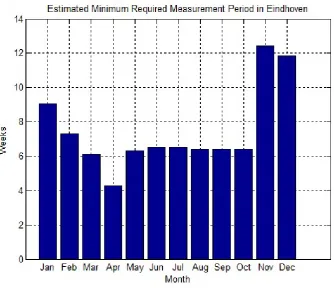
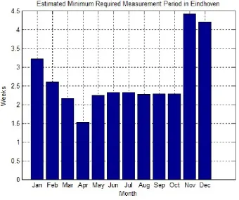
The minimum requirement of measurement duration is providing enough samples for re-liable parameter estimation results. With the theory of sample size estimation [32], the minimum sample size is390for each scenario, if condence interval is0.9 and sampling error

is0.05.

Figure 8.2 shows the estimated minimum measurement duration in Eindhoven, according to 10 years (2001 to 2012) records. To draw reliable conclusions, recommended measurement duration is about 6 weeks. Measurement is not recommended in November, December and January.

(69)

[image:69.595.133.468.255.543.2]

8.2. Recommendations 55

(70)

Mathematical derivation will be listed in Appendix C.

8.3 Future Work

This thesis just intends to provide a methodology to extrapolate internal daylight with short-term measurement and long-term database. According to the issues discussed in the thesis, the future work of this project includes:

• To improve the extrapolation performance, more detailed occupancy information can

be introduced, instead of concluding the occupancy by date;

• Parameter estimation results show that parameters in some scenarios are quite similar,

which provides some approaches to simplify the model;

(71)

Appendix A

Hardware, Software and Data Sources

In this appendix, devices and data sources involved in this project will be introduced, including:

• Wireless daylight monitoring system, which consists of wireless sensor node,

corre-sponding TinyOS project running on the nodes and Building Management Framework (BMF) running on the PC;

• Koninklijk Nederlands Meteorologisch Instituut (KNMI);

• Building Management System (BMS);

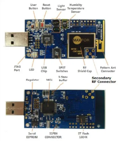
A.1 Wireless Sensor Node

Wireless sensor node involved in this project is CM5000 produced by Advantics. CM5000 node is IEEE 802.15.4 compliant wireless sensor node based on the original open-source "TelosB" [51] [10] platform design developed and published by UC Berkeley. Detailed docu-ment about CM5000 can be found via this link [4].

A picture of CM5000 node is shown in Figure A.1:

The program running on nodes was developed as a TinyOS [11] [36] project. After installing the TinyOS cross-compile tool chain on Ubuntu 10.10 virtual machine, TinyOS project can be compiled and installed on CM5000 by GNU make.

A.2 Building Management Framework

Building Management Framework, which is abbreviated as BMF, is a domain specic framework for exible and ecient distributed sensing and actuation in buildings.

BMF provides run-time node reconguration which allows user to re-deploy and switch applications through conguration packets and exible group organization, which supports setting and change of group aliations for the nodes at run-time. Figure A.2 shows the screenshot of conguring new task for a group of nodes.

After installing and conguring TinyOS project and BMF, wireless daylight monitoring system is ready to be deployed.

(72)

[image:72.595.189.394.104.349.2]

Figure A.1: CM5000 Wireless Sensor Node

[image:72.595.93.489.408.707.2]

(73)

A.3. Koninklijk Nederlands Meteorologisch Instituut (KNMI) 59

[image:73.595.107.505.245.534.2]

A.3 Koninklijk Nederlands Meteorologisch Instituut (KNMI)

Koninklijk Nederlands Meteorologisch Instituut (KNMI, in English: Royal Netherlands Meteorological Institute) is the national institute weather forecasting service in Netherlands [8]. Its primary tasks are forecasting weather and monitoring weather changes. For major cities in Netherlands, KNMI has more than 3 decades' hourly weather condition records which are available online and free to download. Records including temperature, humidity and wind speed etc. The records which related to this project are the hourly solar radiation and cloudiness since 2001 in Eindhoven. Corresponding weather station is Station 370. Location of this station and the proposed building, HTC 34, are shown in Figure A.3.

Figure A.3: KNMI Weather Station 370 (Green Arrow) and High Tech Campus 34 (Marker A)

A.4 Building Management System

(74)

(75)

Appendix B

Results Conversion

In this appendix, Node Result Conversion Formula will be introduced.

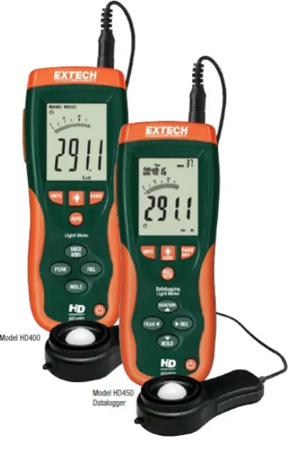
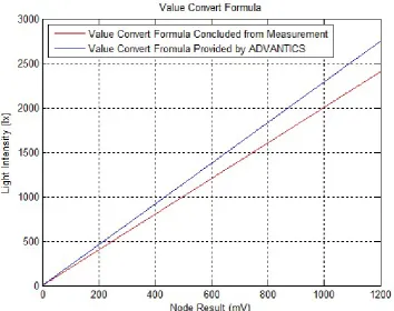
[image:75.595.201.412.326.649.2]

Because CM5000 returns the analog digital converter voltage value as light intensity, a formula is required to convert this value to light intensity (lx). In previous project, the node results (mV) have been measured under dierent light intensity levels. Results was compared with the corresponding light intensity (lx) measured by professional portable lx meter (EXTECH HD450 [6], as shown in Figure B.1).

Figure B.1: EXTECH HD450

Figure B.2 shows the dierence between value convert formulae concluded from test mea-surement and provided by the vendor.

(76)

[image:76.595.107.462.263.543.2]

Test bed and sensor platform for building usage profiling

MASTER THESIS :