Convolutional Neural Network Language Models

Convolutional Neural Network Language Models

Ngoc-Quan Pham and German Kruszewski and Gemma Boleda Center for Mind/Brain Sciences

University of Trento {firstname.lastname}@unitn.it

Abstract

Convolutional Neural Networks (CNNs) have shown to yield very strong results in several Computer Vision tasks. Their application to language has received much less attention, and it has mainly focused on static classifica-tion tasks, such as sentence classificaclassifica-tion for Sentiment Analysis or relation extraction. In this work, we study the application of CNNs to language modeling, a dynamic, sequential prediction task that needs models to capture local as well as long-range dependency infor-mation. Our contribution is twofold. First, we show that CNNs achieve 11-26% better absolute performance than feed-forward neu-ral language models, demonstrating their po-tential for language representation even in se-quential tasks. As for recurrent models, our model outperforms RNNs but is below state of the art LSTM models. Second, we gain some understanding of the behavior of the model, showing that CNNs in language act as feature detectors at a high level of abstraction, like in Computer Vision, and that the model can prof-itably use information from as far as 16 words before the target.

1 Introduction

Convolutional Neural Networks (CNNs) are the family of neural network models that feature a type of layer known as the convolutional layer. This layer can extract features by convolving a learnable filter (or kernel) along different positions of a vectorial in-put.

CNNs have been successfully applied in Com-puter Vision in many different tasks, including

ob-ject recognition, scene parsing, and action recogni-tion (Gu et al., 2015), but they have received less attention in NLP. They have been somewhat ex-plored instatic classification taskswhere the model is provided with a full linguistic unit as input (e.g. a sentence) and classes are treated as independent of each other. Examples of this are sentence or docu-ment classification for tasks such as Sentidocu-ment Anal-ysis or Topic Categorization (Kalchbrenner et al., 2014; Kim, 2014), sentence matching (Hu et al., 2014), and relation extraction (Nguyen and Grish-man, 2015). However, their application to sequen-tial prediction tasks, where the input is construed to be part of a sequence (for example, language model-ing or POS taggmodel-ing), has been rather limited (with exceptions, such as Collobert et al. (2011)). The main contribution of this paper is a systematic evalu-ation of CNNs in the context of a prominent sequen-tial prediction task, namely, language modeling.

Statistical language models are a crucial compo-nent in many NLP applications, such as Automatic Speech Recognition, Machine Translation, and In-formation Retrieval. Here, we study the problem under the standard formulation of learning to predict the upcoming token given its previous context. One successful approach to this problem relies on count-ing the number of occurrences of n-grams while

using smoothing and back-off techniques to esti-mate the probability of an upcoming word (Kneser and Ney, 1995). However, since each individual word is treated independently of the others,n-gram models fail to capture semantic relations between words. In contrast, neural network language mod-els (Bengio et al., 2006) learn to predict the

coming word given the previous context while em-bedding the vocabulary in a continuous space that can represent the similarity structure between words. Both feed-forward (Schwenk, 2007) and recurrent neural networks (Mikolov et al., 2010) have been shown to outperformn-gram models in various

se-tups (Mikolov et al., 2010; Hai Son et al., 2011). These two types of neural networks make different architectural decisions. Recurrent networks take one token at a time together with a hidden “memory” vector as input and produce a prediction and an up-dated hidden vector for the next time step. In con-trast, feed-forward language models take as input the lastntokens, where n is a fixed window size, and

use them jointly to predict the upcoming word. In this paper we define and explore CNN-based language models and compare them with both feed-forward and recurrent neural networks. Our results show a 11-26% perplexity reduction of the CNN with respect to the feed-forward language model, comparable or higher performance compared to similarly-sized recurrent models, and lower perfor-mance with respect to larger, state-of-the-art recur-rent language models (LSTMs as trained in Zaremba et al. (2014)).

Our second contribution is an analysis of the kind of information learned by the CNN, showing that the network learns to extract a combination of grammat-ical, semantic, and topical information from tokens of all across the input window, even those that are the farthest from the target.

2 Related Work

Convolutional Neural Networks (CNNs) were orig-inally designed to deal with hierarchical representa-tion in Computer Vision (LeCun and Bengio, 1995). Deep convolutional networks have been success-fully applied in image classification and understand-ing (Simonyan and Zisserman, 2014; He et al., 2015). In such systems the convolutional kernels learn to detect visual features at both local and more abstract levels.

In NLP, CNNs have been mainly applied to static classification tasks for discovering latent structures in text. Kim (2014) uses a CNN to tackle sentence classification, with competitive results. The same work also introduces kernels with varying window

sizes to learn complementary features at different aggregation levels. Kalchbrenner et al. (2014) pro-pose a convolutional architecture for sentence repre-sentation that vertically stacks multiple convolution layers, each of which can learn independent convo-lution kernels. CNNs with similar structures have also been applied to other classification tasks, such as semantic matching (Hu et al., 2014), relation ex-traction (Nguyen and Grishman, 2015), and infor-mation retrieval (Shen et al., 2014). In contrast, Col-lobert et al. (2011) explore a CNN architecture to solve various sequential and non-sequential NLP tasks such as part-of-speech tagging, named entity recognition and also language modeling. This is per-haps the work that is closest to ours in the existing literature. However, their model differs from ours in that it uses a max-pooling layer that picks the most activated feature across time, thus ignoring tempo-ral information, whereas we explicitly avoid doing so. More importantly, the language models trained in that work are only evaluated through downstream tasks and through the quality of the learned word embeddings, but not on the sequence prediction task itself, as we do here.

Besides being applied to word-based sequences, the convolutional layers have also been used to model sequences at the character level. Kim et al. (2015) propose a recurrent language model that re-places the word-indexed projection matrix with a convolution layer fed with the character sequence that constitutes each word to find morphological pat-terns. The main difference between that work and ours is that we consider words as the smallest lin-guistic unit, and thus apply the convolutional layer at the word level.

Statistical language modeling, the task we tackle, differs from most of the tasks where CNNs have been applied before in multiple ways. First, the input typically consists of incomplete sequences of words rather than complete sentences. Second, as a classi-fication problem, it features an extremely large num-ber of classes (the words in a large vocabulary). Fi-nally, temporal information, which can be safely dis-carded in many settings with little impact in perfor-mance, is critical here: Ann-gram appearing close to the predicted word may be more informative, or yield different information, than the same n-gram

3 Models

Our model is constructed by extending a feed-forward language model (FFLM) with convolutional layers. In what follows, we first explain the imple-mentation of the base FFLM and then describe the CNN model that we study.

3.1 Baseline FFLM

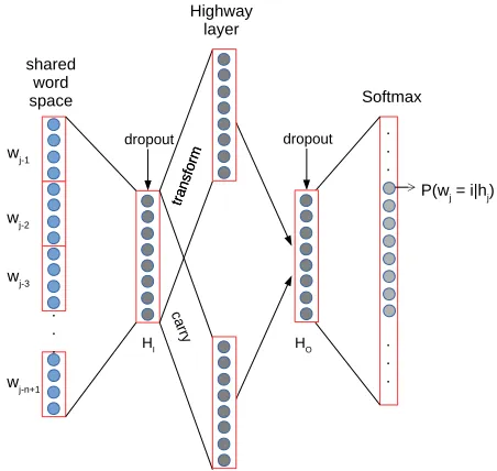
Our baseline feed-forward language model (FFLM) is almost identical to the original model proposed by Bengio et al. (2006), with only slight changes to push its performance as high as we can, producing a very strong baseline. In particular, we extend it with highway layers and use Dropout as regulariza-tion. The model is illustrated in Figure 1 and works as follows. First, each word in the inputn-gram is

mapped to a low-dimensional vector (viz. embed-ding) though a shared lookup table. Next, these word vectors are concatenated and fed to a highway layer (Srivastava et al., 2015). Highway layers im-prove the gradient flow of the network by computing as output a convex combination between its input (called thecarry) and a traditional non-linear trans-formation of it (called thetransform). As a result, if there is a neuron whose gradient cannot flow through the transform component (e.g., because the activa-tion is zero), it can still receive the back-propagaactiva-tion update signal through the carry gate. We empiri-cally observed the usage of a single highway layer to significantly improve the performance of the model. Even though a systematic evaluation of this aspect is beyond the scope of the current paper, our empirical results demonstrate that the resulting model is a very competitive one (see Section 4).

Finally, a softmax layer computes the model pre-diction for the upcoming word. We use ReLU for all non-linear activations, and Dropout (Hinton et al., 2012) is applied between each hidden layer.

3.2 CNN and variants

The proposed CNN network is produced by inject-ing a convolutional layer right after the words in the input are projected to their embeddings (Figure 2). Rather than being concatenated into a long vector, the embeddingsxi ∈Rkare concatenated

transver-sally producing a matrixx1:n ∈ Rn×k, wherenis

1

. . .

. . .

. . . shared

word

space Softmax

P(w_j = i|h_j) wj-1

w_j-n+1

w_j-2

w_j-3

Highway layer

dropout dropout

HI HO

tran sfor

m

ca rry

tran sfor

m

Figure 1:Overview of baseline FFLM.

the size of the input and k is the embedding size. This matrix is fed to a time-delayed layer, which convolves a sliding window ofwinput vectors

cen-tered on each word vector using a parameter matrix

W ∈ Rw×k_{. Convolution is performed by taking}

the dot-product between the kernel matrix W and

each sub-matrix x_{i−w/2:i+w/2} resulting in a scalar value for each positioniin input context. This value

represents how much the words encompassed by the window match the feature represented by the filter

W. A ReLU activation function is applied

subse-quently so negative activations are discarded. This operation is repeated multiple times using various kernel matrices W, learning different features

in-dependently. We tie the number of learned kernels to be the same as the embedding dimensionalityk,

such that the output of this stage will be another ma-trix of dimensionsn_×kcontaining the activations

for each kernel at each time step. The number of kernels was tied to the embedding size for two rea-sons, one practical, namely, to limit the hyper pa-rameter search, one methodological, namely, to keep the network structure identical to that of the baseline feed-forward model.

shift problem and regularizing the learned represen-tations (Ioffe and Szegedy, 2015).

Finally, this feature matrix is directly fed into a fully connected layer that can project the ex-tracted features into a lower-dimensional represen-tation. This is different from previous work, where a max-over-time pooling operation was used to find the most activated feature in the time series. Our choice is motivated by the fact that the max pooling operator loses the specific position where the feature was detected, which is important for word predic-tion.

After this initial convolutional layer, the network proceeds identically to the FFNN by feeding the pro-duced features into a highway layer, and then, to a softmax output.

This is our basic CNN architecture. We also ex-periment with three expansions to the basic model, as follows. First, we generalize the CNN by ex-tending the shallow linear kernels with deeper multi-layer perceptrons, in what is called a MLP Convolu-tion (MLPConv) structure (Lin et al., 2013). This allows the network to produce non-linear filters, and it has achieved state-of-the-art performance in object recognition while reducing the number of total lay-ers compared to other mainstream networks. Con-cretely, we implement MLPConv networks by using another convolutional layer with a1×1 kernel on

top of the convolutional layer output. This results in an architecture that is exactly equivalent to sliding a one-hidden-layer MLP over the input. Notably, we do not include the global pooling layer in the origi-nal Network-in-Network structure (Lin et al., 2013). Second, we explore stacking convolutional lay-ers on top of each other (Multi-layer CNN or ML-CNN) to connect the local features into broader re-gional representations, as commonly done in com-puter vision. While this proved to be useful for sentence representation (Kalchbrenner et al., 2014), here we have found it to be rather harmful for lan-guage modeling, as shown in Section 4. It is impor-tant to note that, in ML-CNN experiments, we stack convolutions with the same kernel size and number of kernels on top of each other, which is to be distin-guished from the MLPConv that refers to the deeper structure in each CNN layer mentioned above.

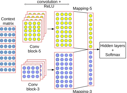
Finally, we consider combining features learned through different kernel sizes (COM), as depicted in

1

Hidden layers + Softmax context

matrix

Convolution + ReLU

Mapping

Figure 2:Convolutional layer on top of the context matrix.

Context matrix

convolution + ReLU

Conv block-5

Conv block-3

Mapping-5

Mapping-3

Hidden layers + Softmax

Figure 3:Combining kernels with different sizes. We concate-nate the outputs of 2 convolutional blocks with kernel size of5

and3respectively.

Figure 3. For example, we can have a combination of kernels that learn filters over 3-grams with oth-ers that learn over 5-grams. This is achieved simply by applying in parallel two or more sets of kernels to the input and concatenating their respective out-puts (Kim, 2014).

4 Experiments

We evaluate our model on three English corpora of different sizes and genres, the first two of which have been used for language modeling evaluation

before. The Penn Treebank contains one

al. (2014). Europarl-NCis a 64-million word cor-pus that was developed for a Machine Translation shared task (Bojar et al., 2015), combining Europarl data (from parliamentary debates in the European Union) and News Commentary data. We prepro-cessed the corpus with tokenization and true-casing tools from the Moses toolkit (Koehn et al., 2007). The vocabulary is composed of words that occur at least 3 times in the training set and contains approx-imately 60K words. We use the validation and test set of the MT shared task. Finally, we took a sub-set of the ukWaC corpus, which was constructed by crawling UK websites (Baroni et al., 2009). The training subset contains 200 million words and the vocabulary consists of the 200K words that appear more than 5 times in the training subset. The val-idation and test sets are different subsets of the ukWaC corpus, both containing 120K words. We preprocessed the data similarly to what we did for Europarl-NC.

We train our models using Stochastic Gradient Descent (SGD), which is relatively simple to tune compared to other optimization methods that involve additional hyper parameters (such as alpha in RM-Sprop) while being still fast and effective. SGD is commonly used in similar work (Devlin et al., 2014; Zaremba et al., 2014; Sukhbaatar et al., 2015). The learning rate is kept fixed during a single epoch, but we reduce it by a fixed proportion every time the val-idation perplexity increases by the end of the epoch. The values for learning rate, learning rate shrinking and mini-batch sizes as well as context size are fixed once and for all based on insights drawn from pre-vious work (Hai Son et al., 2011; Sukhbaatar et al., 2015; Devlin et al., 2014) as well as experimentation with the Penn Treebank validation set.

Specifically, the learning rate is set to 0.05, with mini-batch size of 128 (we do not take the average of loss over the batch, and the training set is shuffled). We multiply the learning rate by 0.5 every time we shrink it and clip the gradients if their norm is larger than 12. The network parameters are initialized ran-domly on a range from -0.01 to 0.01 and the context size is set to 16. In Section 6 we show that this large context window is fully exploited.

For the base FFNN and CNN we varied em-bedding sizes (and thus, number of kernels) k = 128,256. Fork= 128we explore the simple CNN,

incrementally adding MLPConv and COM varia-tions (in that order) and, alternatively, using a ML-CNN. For k = 256, we only explore the former

three alternatives (i.e. all but the ML-CNN). For the kernel size, we set it to w = 3words for the

sim-ple CNN (out of options3,5,7,9), whereas for the

COM variant we usew= 3and5, based on

experi-mentation on PTB. However, we observed the mod-els to be generally robust to this parameter. Dropout rates are tuned specifically for each combination of model and dataset based on the validation perplex-ity. We also add small dropout (p = 0.05–0.15) when we train the networks on the smaller corpus (Penn Treebank).

The experimental results for recurrent neural net-work language models, such as Recurrent Neural Networks (RNN) and Long-Short Term Memory models (LSTM), on the Penn Treebank are quoted from previous work; for Europarl-NC, we train our own models (we also report the performance of these in-house trained RNN and LSTM models on the Penn Treebank for reference). Specifically, we train LSTMs with embedding sizek = 256and number of layersL = 2as well ask = 512withL = 1,2.

We train one RNN withk= 512andL= 2. To train

these models, we use the published source code from Zaremba et al. (2014). Our own models are also implemented in Torch7 for easier comparison.1 Fi-nally, we selected the best performing convolutional and recurrent language models on Europarl-NC and the Baseline FFLM to be evaluated on the ukWaC corpus.

For all models trained on Europarl-NC and ukWaC, we speed up training by approximating the softmax with Noise Contrastive Estimation (NCE) (Gutmann and Hyv¨arinen, 2010), with the parameters being set following previous work (Chen et al., 2015). Concretely, for each predicted word, we sample 10 words from the unigram distribution, and the normalization factor is such thatlnZ = 9.2 For comparison, we also implemented a simpler version of the FFNN without dropout and highway layers (Bengio et al., 2006). These networks have two hidden layers (Arisoy et al., 2012) with the size 1_{Available at https://github.com/quanpn90/NCE CNNLM.} 2_{We also experimented with Hierarchical Softmax (Mikolov}

of 2 times the embedding size (k), thus having the

same number of parameters as our baseline.

5 Results

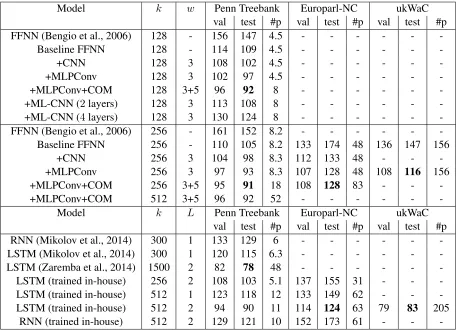
Our experimental results are summarized in Table 1. First of all, we can see that, even though the FFNN gives a very competitive performance,3 _the addition of convolutional layers clearly improves it even further. Concretely, we observe a solid 11-26% reduction of perplexity compared to the feed-forward network after using MLP Convolution, depending on the setup and corpus. CNN alone yields a sizable improvement (5-24%), while MLP-Conv, in line with our expectations, adds another approximately 2-5% reduction in perplexity. A fi-nal (smaller) improvement comes from combining kernels of size 3 and 5, which can be attributed to a more expressive model that can learn patterns of

n-grams of different sizes. In contrast to the

suc-cessful two variants above, the multi-layer CNN did not help in better capturing the regularities of text, but rather the opposite: the more convolutional lay-ers were stacked, the worse the performance. This also stands in contrast to the tradition of convolu-tional networks in Computer Vision, where using very deep convolutional neural networks is key to having better models. Deep convolution for text representation is in contrast rather rare, and to our knowledge it has only been successfuly applied to sentence representation (Kalchbrenner et al., 2014). We conjecture that the reason why deep CNNs may not be so effective for language could be the effect of the convolution on the data: The convolution output for an image is akin to a new, more abstract image, which yet again can be subject to new convolution operations, whereas the textual counterpart may no longer have the same properties, in the relevant as-pects, as the original linguistic input.

Regarding the comparison with a stronger LSTM, our models can perform competitively under the same embedding dimension (e.g. see k = 256 of

k = 512) on the first two datasets. However, the

LSTM can be easily scaled using larger models, as shown in Zaremba et al. (2014), which gives the

3_{In our experiments, increasing the number of fully}

con-nected layers of the FFNN is harmful. Two hidden layers with highway connections is the best setting we could find.

best known results to date. This is not an option for our model, which heavily overfits with large hidden layers (around 1000) even with very large dropout values. Furthermore, the experiments on the larger ukWaC corpus show an even clearer advantage for the LSTM, which seems to be more efficient at har-nessing this volume of data, than in the case of the two smaller corpora.

To sum up, we have established that the results of our CNN model are well above those of sim-ple feed forward networks and recurrent neural net-works. While they are below state of the art LSTMs, they are able to perform competitively with them for small and moderate-size models. Scaling to larger sizes may be today the main roadblock for CNNs to reach the same performances as large LSTMs in language modeling.

6 Model Analysis

In what follows, we obtain insights into the inner workings of the CNN by looking into the linguis-tic patterns that the kernels learn to extract and also studying the temporal information extracted by the network in relation to its prediction capacity.

Model k w Penn Treebank Europarl-NC ukWaC

val test #p val test #p val test #p

FFNN (Bengio et al., 2006) 128 - 156 147 4.5 - - -

-Baseline FFNN 128 - 114 109 4.5 - - -

-+CNN 128 3 108 102 4.5 - - -

-+MLPConv 128 3 102 97 4.5 - - -

-+MLPConv+COM 128 3+5 96 92 8 - - -

-+ML-CNN (2layers) 128 3 113 108 8 - - -

-+ML-CNN (4layers) 128 3 130 124 8 - - -

-FFNN (Bengio et al., 2006) 256 - 161 152 8.2 - - -

-Baseline FFNN 256 - 110 105 8.2 133 174 48 136 147 156

+CNN 256 3 104 98 8.3 112 133 48 - -

-+MLPConv 256 3 97 93 8.3 107 128 48 108 116 156

+MLPConv+COM 256 3+5 95 91 18 108 128 83 - -

-+MLPConv+COM 512 3+5 96 92 52 - - -

-Model k L Penn Treebank Europarl-NC ukWaC

val test #p val test #p val test #p

RNN (Mikolov et al., 2014) 300 1 133 129 6 - - -

-LSTM (Mikolov et al., 2014) 300 1 120 115 6.3 - - -

-LSTM (Zaremba et al., 2014) 1500 2 82 78 48 - - -

-LSTM (trained in-house) 256 2 108 103 5.1 137 155 31 - -

-LSTM (trained in-house) 512 1 123 118 12 133 149 62 - -

-LSTM (trained in-house) 512 2 94 90 11 114 124 63 79 83 205

RNN (trained in-house) 512 2 129 121 10 152 173 61 - -

-Table 1:Results on Penn Treebank and Europarl-NC. Figure of merit is perplexity (lower is better). Legend:k: embedding size (also number of kernels for the convolutional models and hidden layer size for the recurrent models);w: kernel size;val: results on validation data;test: results on test data;#p: number of parameters in millions;L: number of layers.

no matter how are afraid how question is how remaining are how

to say how

as little as of more than

as high as as much as

as low as

a merc spokesman a company spokesman

a boeing spokesman a fidelity spokesman a quotron spokeswoman

amr chairman robert chief economist john chicago investor william exchange chairman john

texas billionaire robert

would allow the does allow the still expect ford warrant allows the funds allow investors

more evident among a dispute among bargain-hunting among

growing fear among paintings listed among

facilities will substantially which would substantially

dean witter actually we 'll probably you should really

have until nov. operation since aug. quarter ended sept. terrible tuesday oct. even before june

Figure 4:Some example phrases that have highest activations for 8 example kernels (each box), extracted from the validation set of the Penn Treebank. Model trained with 256 kernels for 256-dimensional word vectors.

abstraction” dimension to a feed-forward neural net-work, similarly to what has been observed in image classification (Krizhevsky et al., 2012).

110 120 130 140 150 160 170 180 190 200 210

0 2 4 6 8 10 12 14 16

Sum of positive weights

Positions

Figure 5:The distribution of positive weights over context po-sitions, where 1 is the position closest to the predicted word.

where no significant change in terms of perplexity was observed for bigger context sizes, even though in that work only same-sentence contexts were con-sidered. In our experiments, we use a larger context size of 16 while removing the sentence boundary limit (as commonly done inn-gram language

mod-els) such that the network can take into account the words in the previous sentences.

To analyze whether all this information was effectively used, we took our best model, the CNN+MLPConv+COM model with embedding size of 256 (fifth line of second block in Table 1), and we identified the weights in the model that map the convolutional output (of sizen×k) to a lower

di-mensional vector (the “mapping” layer in Figure 2). Recall that the output of the convolutional layer is a matrix indexed by time step and kernel index con-taining the activation of the kernel when convolved with a window of text centered around the word at the given time step. Thus, output units of the above mentioned mapping predicate over an ensem-ble of kernel activations for each time step. We can identify the patterns that they learn to detect by extracting the time-kernel combinations for which they have positive weights (since we have ReLU ac-tivations, negative weights are equivalent to ignor-ing a feature). First, we asked ourselves whether these units tend to be more focused on the time steps closer to the target or not. To test this, we calculated the sum of the positive weights for each position in time using an average of the mappings that corre-spond to each output unit. The results are shown in

4.5 5 5.5 6 6.5 7

0 2 4 6 8 10 12 14 16

Cross Entropy

Number of positions revealed

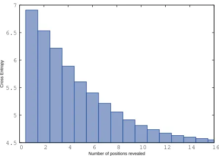
Figure 6:Perplexity change over position, by incrementally re-vealing the Mapping’s weights corresponding to each position.

Figure 5. As could be expected, positions that are close to the token to be predicted have many active units (local context is very informative; see positions 2-4). However, surprisingly, positions that are actu-ally far from the target are also quite active. It seems like the CNN is putting quite a lot of effort on char-acterizing long-range dependencies.

Next, we checked that the information extracted from the positions that are far in the past are actu-ally used for prediction. To measure this, we arti-ficially lesioned the network so it would only read the features from a given range of time steps (words in the context). To lesion the network we manually masked the weights of the mapping that focus on times outside of the target range by setting them to zero. We started using only the word closest to the final position and sequentially unmasked earlier po-sitions until the full context was used again. The re-sult of this experiment is presented in Figure 6, and it confirms our previous observation that positions that are the farthest away contribute to the predic-tions of the model. The perplexity drops dramati-cally as the first positions are unmasked, and then decreases more slowly, approximately in the form of a power law (f(x)∝x−0.9). Even though the

ef-fect is smaller, the last few positions still contribute to the final perplexity.

7 Conclusion

predic-tion task. We incorporate a CNN layer on top of a strong feed-forward model enhanced with modern techniques like Highway Layers and Dropout. Our results show a solid 11-26% reduction in perplexity with respect to the feed-forward model across three corpora of different sizes and genres when the model uses MLP Convolution and combines kernels of dif-ferent window sizes. However, even without these additions we show CNNs to effectively learn lan-guage patterns that allow it to significantly decrease the model perplexity.

In our view, this improvement responds to two key properties of CNNs, highlighted in the analysis. First, as we have shown, they are able to integrate information from larger context windows, using in-formation from words that are as far as 16 positions away from the predicted word. Second, as we have qualitatively shown, the kernels learn to detect spe-cific patterns at a high level of abstraction. This is analogous to the role of convolutions in Computer Vision. The analogy, however, has limits; for in-stance, a deeper model stacking convolution layers harms performance in language modeling, while it greatly helps in Computer Vision. We conjecture that this is due to the differences in the nature of vi-sual vs. linguistic data. The convolution creates sort of abstract images that still retain significant proper-ties of images. When applied to language, it detects important textual features but distorts the input, such that it is not text anymore.

As for recurrent models, even if our model out-performs RNNs, it is well below state-of-the-art LSTMs. Since CNNs are quite different in nature, we believe that a fruitful line of future research could focus on integrating the convolutional layer into a recurrent structure for language modeling, as well as other sequential problems, perhaps capturing the best of both worlds.

Acknowledgments

We thank Marco Baroni and three anonymous viewers for fruitful feedback. This project has re-ceived funding from the European Union’s Hori-zon 2020 research and innovation programme un-der the Marie Sklodowska-Curie grant agreement No 655577 (LOVe); ERC 2011 Starting Independent Research Grant n. 283554 (COMPOSES) and the

Erasmus Mundus Scholarship for Joint Master Pro-grams. We gratefully acknowledge the support of NVIDIA Corporation with the donation of the GPUs used in our research.

References

Ebru Arisoy, Tara N Sainath, Brian Kingsbury, and Bhu-vana Ramabhadran. 2012. Deep neural network lan-guage models. In Proceedings of the NAACL-HLT 2012 Workshop: Will We Ever Really Replace the N-gram Model? On the Future of Language Modeling for HLT, pages 20–28. Association for Computational Linguistics.

Marco Baroni, Silvia Bernardini, Adriano Ferraresi, and Eros Zanchetta. 2009. The WaCky wide web: A collection of very large linguistically processed web-crawled corpora. Language Resources and Evalua-tion, 43(3):209–226.

Yoshua Bengio, Holger Schwenk, Jean-S´ebastien Sen´ecal, Fr´ederic Morin, and Jean-Luc Gauvain. 2006. Neural probabilistic language models. In Innovations in Machine Learning, pages 137–186. Springer.

Ondˇrej Bojar, Rajen Chatterjee, Christian Federmann, Barry Haddow, Matthias Huck, Chris Hokamp, Philipp Koehn, Varvara Logacheva, Christof Monz, Matteo Negri, Matt Post, Carolina Scarton, Lucia Specia, and Marco Turchi. 2015. Findings of the 2015 workshop on statistical machine translation. InProceedings of the Tenth Workshop on Statistical Machine Transla-tion, pages 1–46, Lisbon, Portugal, September. Asso-ciation for Computational Linguistics.

Xie Chen, Xunying Liu, Mark JF Gales, and Philip C Woodland. 2015. Recurrent neural network language model training with noise contrastive estimation for speech recognition. In2015 IEEE International Con-ference on Acoustics, Speech and Signal Processing (ICASSP), pages 5411–5415. IEEE.

Ronan Collobert, Jason Weston, L´eon Bottou, Michael Karlen, Koray Kavukcuoglu, and Pavel Kuksa. 2011. Natural language processing (almost) from scratch. The Journal of Machine Learning Research, 12:2493– 2537.

Jacob Devlin, Rabih Zbib, Zhongqiang Huang, Thomas Lamar, Richard M Schwartz, and John Makhoul. 2014. Fast and robust neural network joint models for statistical machine translation. InACL (1), pages 1370–1380. Citeseer.

ad-vances in convolutional neural networks. CoRR, abs/1512.07108.

Michael Gutmann and Aapo Hyv¨arinen. 2010. Noise-contrastive estimation: A new estimation principle for unnormalized statistical models. In AISTATS, vol-ume 1, page 6.

Le Hai Son, Ilya Oparin, Alexandre Allauzen, Jean-Luc Gauvain, and Franc¸ois Yvon. 2011. Structured output layer neural network language model. In Acoustics, Speech and Signal Processing (ICASSP), 2011 IEEE International Conference on, pages 5524–5527. IEEE. Le Hai Son, Alexandre Allauzen, and Franc¸ois Yvon. 2012. Measuring the influence of long range depen-dencies with neural network language models. In Pro-ceedings of the NAACL-HLT 2012 Workshop: Will We Ever Really Replace the N-gram Model? On the Fu-ture of Language Modeling for HLT, pages 1–10. As-sociation for Computational Linguistics.

Kaiming He, Xiangyu Zhang, Shaoqing Ren, and Jian Sun. 2015. Deep residual learning for image recogni-tion. arXiv preprint arXiv:1512.03385.

Geoffrey E. Hinton, Nitish Srivastava, Alex Krizhevsky, Ilya Sutskever, and Ruslan Salakhutdinov. 2012. Im-proving neural networks by preventing co-adaptation of feature detectors. CoRR, abs/1207.0580.

Baotian Hu, Zhengdong Lu, Hang Li, and Qingcai Chen. 2014. Convolutional neural network architectures for matching natural language sentences. InAdvances in Neural Information Processing Systems, pages 2042– 2050.

Sergey Ioffe and Christian Szegedy. 2015. Batch normalization: Accelerating deep network training by reducing internal covariate shift. arXiv preprint arXiv:1502.03167.

Nal Kalchbrenner, Edward Grefenstette, and Phil Blun-som. 2014. A convolutional neural network for mod-elling sentences. InProceedings of the 52nd Annual Meeting of the Association for Computational Linguis-tics, ACL 2014, June 22-27, 2014, Baltimore, MD, USA, Volume 1: Long Papers, pages 655–665. Yoon Kim, Yacine Jernite, David Sontag, and

Alexan-der M. Rush. 2015. Character-aware neural language models. CoRR.

Yoon Kim. 2014. Convolutional neural networks for sen-tence classification. arXiv preprint arXiv:1408.5882. Reinhard Kneser and Hermann Ney. 1995. Improved

backing-off for m-gram language modeling. In Acous-tics, Speech, and Signal Processing, 1995. ICASSP-95., 1995 International Conference on, volume 1, pages 181–184. IEEE.

Philipp Koehn, Hieu Hoang, Alexandra Birch, Chris Callison-Burch, Marcello Federico, Nicola Bertoldi, Brooke Cowan, Wade Shen, Christine Moran, Richard

Zens, et al. 2007. Moses: Open source toolkit for statistical machine translation. InProceedings of the 45th annual meeting of the ACL on interactive poster and demonstration sessions, pages 177–180. Associa-tion for ComputaAssocia-tional Linguistics.

Alex Krizhevsky, Ilya Sutskever, and Geoffrey E Hinton. 2012. Imagenet classification with deep convolutional neural networks. In Advances in neural information processing systems, pages 1097–1105.

Yann LeCun and Yoshua Bengio. 1995. Convolu-tional networks for images, speech, and time series. The handbook of brain theory and neural networks, 3361(10):1995.

Min Lin, Qiang Chen, and Shuicheng Yan. 2013. Net-work in netNet-work. arXiv preprint arXiv:1312.4400. Tomas Mikolov, Martin Karafi´at, Lukas Burget, Jan

Cer-nock`y, and Sanjeev Khudanpur. 2010. Recurrent neural network based language model. In INTER-SPEECH, volume 2, page 3.

Tom´aˇs Mikolov, Stefan Kombrink, Luk´aˇs Burget, Jan Honza ˇCernock`y, and Sanjeev Khudanpur. 2011. Extensions of recurrent neural network language model. In Acoustics, Speech and Signal Processing (ICASSP), 2011 IEEE International Conference on, pages 5528–5531. IEEE.

Tomas Mikolov, Armand Joulin, Sumit Chopra, Michael Mathieu, and Marc’Aurelio Ranzato. 2014. Learning longer memory in recurrent neural networks. arXiv preprint arXiv:1412.7753.

Thien Huu Nguyen and Ralph Grishman. 2015. Relation extraction: Perspective from convolutional neural net-works. InProceedings of NAACL-HLT, pages 39–48. Holger Schwenk. 2007. Continuous space language

models. Computer Speech & Language, 21(3):492– 518.

Yelong Shen, Xiaodong He, Jianfeng Gao, Li Deng, and Gr´egoire Mesnil. 2014. A latent semantic model with convolutional-pooling structure for information retrieval. In Proceedings of the 23rd ACM Interna-tional Conference on Conference on Information and Knowledge Management, pages 101–110. ACM. Karen Simonyan and Andrew Zisserman. 2014. Very

deep convolutional networks for large-scale image recognition.arXiv preprint arXiv:1409.1556.

Rupesh Kumar Srivastava, Klaus Greff, and J¨urgen Schmidhuber. 2015. Highway networks. CoRR, abs/1505.00387.

Sainbayar Sukhbaatar, Jason Weston, Rob Fergus, et al. 2015. End-to-end memory networks. InAdvances in Neural Information Processing Systems, pages 2431– 2439.