Random Forests in Language Modelin

Random Forests in Language Modeling

Peng Xu and Frederick Jelinek

Center for Language and Speech Processing the Johns Hopkins University

Baltimore, MD 21218, USA xp,jelinek @jhu.edu

Abstract

In this paper, we explore the use of Random Forests (RFs) (Amit and Geman, 1997; Breiman, 2001) in language modeling, the problem of predicting the next word based on words already seen before. The goal in this work is to develop a new language mod-eling approach based on randomly grown Decision Trees (DTs) and apply it to automatic speech recog-nition. We study our RF approach in the context of -gram type language modeling. Unlike

regu-lar -gram language models, RF language models

have the potential to generalize well to unseen data, even when a complicated history is used. We show that our RF language models are superior to regular

-gram language models in reducing both the

per-plexity (PPL) and word error rate (WER) in a large vocabulary speech recognition system.

1 Introduction

In many systems dealing with natural speech or lan-guage, such as Automatic Speech Recognition and Statistical Machine Translation, a language model is a crucial component for searching in the often prohibitively large hypothesis space. Most state-of-the-art systems use -gram language models, which

are simple and effective most of the time. Many smoothing techniques that improve language model probability estimation have been proposed and stud-ied in the -gram literature (Chen and Goodman,

1998). There has also been work in exploring Deci-sion Tree (DT) language models (Bahl et al., 1989; Potamianos and Jelinek, 1998), which attempt to cluster similar histories together to achieve better probability estimation. However, the results were not promising (Potamianos and Jelinek, 1998): in a fair comparison, decision tree language models failed to improve upon the baseline -gram models

with the same order .

The aim of DT language models is to alleviate the data sparseness problem encountered in -gram

language models. However, the cause of the neg-ative results is exactly the same: data sparseness,

coupled with the fact that the DT construction al-gorithms decide on tree splits solely on the basis of seen data (Potamianos and Jelinek, 1998). Al-though various smoothing techniques were studied in the context of DT language models, none of them resulted in significant improvements over -gram

models.

Recently, a neural network based language mod-eling approach has been applied to trigram lan-guage models to deal with the curse of dimension-ality (Bengio et al., 2001; Schwenk and Gauvain, 2002). Significant improvements in both perplex-ity (PPL) and word error rate (WER) over backoff smoothing were reported after interpolating the neu-ral network models with the baseline backoff mod-els. However, the neural network models rely on interpolation with -gram models, and use -gram

models exclusively for low frequency words. We believe improvements in -gram models should also

improve the performance of neural network models. We propose a new Random Forest (RF) approach for language modeling. The idea of using RFs for language modeling comes from the recent success of RFs in classification and regression (Amit and Geman, 1997; Breiman, 2001; Ho, 1998). By defi-nition, RFs are collections of Decision Trees (DTs) that have been constructed randomly. Therefore, we also propose a new DT language model which can be randomized to construct RFs efficiently. Once constructed, the RFs function as a randomized his-tory clustering which can help in dealing with the data sparseness problem. Although they do not per-form well on unseen test data individually, the col-lective contribution of all DTs makes the RFs gen-eralize well to unseen data. We show that our RF approach for -gram language modeling can result

in a significant improvement in both PPL and WER in a large vocabulary speech recognition system.

Sec-tion 4, we show the performance of our RF based language models as measured by both PPL and WER. After some discussion and analysis, we fi-nally summarize our work and propose some future directions in Section 5.

2 Basic Language Modeling

The purpose of a language model is to estimate the probability of a word string. Let denote a string of words, that is, . Then,

by the chain rule of probability, we have

"!$#% &('*) ( & + ,.-0/0/0/- &21 3/ (1)

In order to estimate the probabilities

465

87:9 87<; >=, we need a training corpus

consisting of a large number of words. However, in any practical natural language system with even a moderate vocabulary size, it is clear that as ?

increases the accuracy of the estimated probabilities collapses. Therefore, histories @

7<; for

word

7 are usually grouped into equivalence

classes. The most widely used language models,

-gram language models, use the identities of the

last BAC words as equivalence classes. In an

-gram model, we then have

"!$#% &'D) ( & + &21 &E1FHG 3-(2)

where we have used 7<;

7<;JIK to denote the word

se-quence 7<;JIK L 7M; .

The maximum likelihood (ML) estimate of

465 7 9 7<; 7<;JIK = is ( & + &21 &E1FHG M8N$OQP & &21RF>G "S N$OQP &21 &21RF>G S -(3) whereT 5 7 7M;JIRK

= is the number of times the string 7<;JIK L 7 is seen in the training data.

2.1 Language Model Smoothing

An -gram model when UWV is called a trigram

model. For a vocabulary of size90X9*YCZ*[ , there are

90X\9]^_CZ `

trigram probabilities to be estimated. For any training data of a manageable size, many of the probabilities will be zero if the ML estimate is used.

In order to solve this problem, many smoothing techniques have been studied (see (Chen and Good-man, 1998) and the references therein). Smooth-ing adjusts the ML estimates to produce more ac-curate probabilities and to assign nonzero prob-abilies to any word string. Details about vari-ous smoothing techniques will not be presented in this paper, but we will outline a particular way

of smoothing, namely, interpolated Kneser-Ney smoothing (Kneser and Ney, 1995), for later refer-ence.

The interpolated Kneser-Ney smoothing assumes the following form:

ba % ( & + &21 &E1FHG dcfe g OQNhOQP & &E1FHG S 1bijk S N$OQP &21 &21RF>G S Kl &21 &21RF>G Eba % & + &21 &21RF>GD) (4)

wherem is a discounting constant and n

5 7<; 7M;JIRK =

is the interpolation weight for the lower order prob-abilities (

5

oApC =-gram). The discount constant is

often estimated using leave-one-out, leading to the approximation m_

I

I

K I

) , where

q is the

num-ber of -grams with count one and is the number

of -grams with count two. To ensure that the

prob-abilities sum to one, we have

l ( &E1 &21RF>G isr P & t NhOQP & &E1FHG Su k N$OQP &21 &21RF>G S /

The lower order probabilities in interpolated Kneser-Ney smoothing can be estimated as (assum-ing ML estimation):

ba % & + &21 &21RF>GD) M r P &21RF>G t NhO0P & &E1FHG Su k r P &21RF>G j P & t NhO0P & &E1FHG Su k / (5)

Note that the lower order probabilities are usually smoothed using recursions similar to Equation 4.

2.2 Language Model Evalution

A commonly used task-independent quality mea-sure for a given language model is related to the cross entropy of the underlying model and was in-troduced under the name of perplexity (PPL) (Je-linek, 1997): ,,v$w`xzy ; |{ ~} % &' L0€ ƒ‚ ( & + &21 2„3-(6)

where is the test text that consists of

words.

For different tasks, there are different task-dependent quality measures of language models. For example, in an automatic speech recognition system, the performance is usually measured by word error rate (WER).

3 Decision Tree and Random Forest

Language Modeling

RF is a collection of randomly constructed Deci-sion Trees (DTs) (Breiman et al., 1984). Therefore, in order to use RFs for language modeling, we first need to construct DT language models.

3.1 Decision Tree Language Modeling

In an -gram language model, a word sequence

7<;JIK L 7M; is called a history for predicting 7. A DT language model uses a decision tree to

classify all histories into equivalence classes and each history in the same equivalence class shares the same distribution over the predicted words. The idea of DTs has been very appealing in language modeling because it provides a natural way to deal with the data sparseness problem. Based on statis-tics from some training data, a DT is usually grown until certain criteria are satisfied. Heldout data can be used as part of the stopping criterion to determine the size of a DT.

There have been studies of DT language mod-els in the literature. Most of the studies focused on improving -gram language models by

adopt-ing various smoothadopt-ing techniques in growadopt-ing and using DTs (Bahl et al., 1989; Potamianos and Je-linek, 1998). However, the results were not satisfac-tory. DT language models performed similarly to traditional -gram models and only slightly better

when combined with -gram models through

lin-ear interpolation. Furthermore, no study has been done taking advantage of the “best” stand-alone smoothing technique, namely, interpolated Kneser-Ney smoothing (Chen and Goodman, 1998).

The main reason why DT language models are not successful is that algorithms constructing DTs suffer certain fundamental flaws by nature: training data fragmentation and the absence of a theoretically-founded stopping criterion. The data fragmentation problem is severe in DT language modeling because the number of histories is very large (Jelinek, 1997). Furthermore, DT growing al-gorithms are greedy and early termination can oc-cur.

3.1.1 Our DT Growing Algorithm

In recognition of the success of Kneser-Ney (KN) back-off for -gram language modeling (Kneser

and Ney, 1995; Chen and Goodman, 1998), we use a new DT growing procedure to take advantage of KN smoothing. At the same time, we also want to deal with the early termination problem. In our pro-cedure, training data is used to grow a DT until the maximum possible depth, heldout data is then used to prune the DT similarly as in CART (Breiman et al., 1984), and KN smoothing is used in the pruning. A DT is grown through a sequence of node

split-ting. A node consists of a set of histories and a node splitting splits the set of histories into two subsets based on statistics from the training data. Initially, we put all histories into one node, that is, into the root and the only leaf of a DT. At each stage, one of the leaves of the DT is chosen for splitting. New nodes are marked as leaves of the tree. Since our splitting criterion is to maximize the log-likelihood of the training data, each split uses only statistics (from training data) associated with the node under consideration. Smoothing is not needed in the split-ting and we can use a fast exchange algorithm (Mar-tin et al., 1998) to accomplish the task. This can save the computation time relative to the Chou al-gorithm (Chou, 1991) described in Jelinek,1998 (Je-linek, 1997).

Let us assume that we have a DT node under consideration for splitting. Denote by

5

= the set of

all histories seen in the training data that can reach node . In the context of -gram type of modeling,

there are A C items in each history. A position

in the history is the distance between a word in the history and the predicted word. We only consider splits that concern a particular position in the his-tory. Given a position? in the history, we can define

7

5

= to be the set of histories belonging to , such

that they all have word

at position ? . It is clear

that

5

=

7

5

= for every position ? in the

his-tory. For every ?, our algorithm uses

7

5

= as basic

elements to construct two subsets, 7 and 7

1_{, to}

form the basis of a possible split. Therefore, a node contains two questions about a history: (1) Is the history in 7? and (2) Is the history in 7? If a

his-tory has an answer “yes” to (1), it will proceed to the left child of the node. Similarly, if it has an answer “yes” to (2), it will proceed to the right child. If the answers to both questions are “no”, the history will not proceed further.

For simplicity, we omit the subscript? in later

dis-cussion since we always consider one position at a time. Initially, we split

5

= into two non-empty

disjoint subsets, and , using the elements 5

=.

Let us denote the log-likelihood of the training data associated with under the split as

5

=. If we use

the ML estimates for probabilities, we will have

v h

}

P

( -h N$OQP

j S

NhO S

K

( - NhO0P

j S

N$O S

}

P

‚

-$

( -h

K

( -

( - 2„

;

h

h

;

(7)

whereT

5

= is the count of word following all

histories in () and T 5

= is the corresponding total

1

&! #"&%$'&)(+*-, and

&/.#"&0$21

count. Note that only counts are involved in Equa-tion 7, an efficient data structure can be used to store them for the computation. Then, we try to find the best subsets and by tentatively moving

ele-ments in to and vice versa. Suppose

5

=

is the element we want to move. The log-likelihood after we move 5

= from to can be calculated

using Equation 7 with the following changes:

-$ -h ;

( -D

M ( - - K

( -D

h h ; D M K D M (8)

If a tentative move results in an increase in log-likelihood, we will accept the move and modify the counts. Otherwise, the element stays where it was. The subsets and are updated after each move.

The algorithm runs until no move can increase the log-likelihood. The final subsets will be and

and we save the total log-likelihood increase. After all positions in the history are examined, we choose the one with the largest increase in log-likelihood for splitting the node. The exchange algorithm is different from the Chou algorithm (Chou, 1991) in the following two aspects: First, unlike the Chou algorithm, we directly use the log-likelihood of the training data as our objective function. Second, the statistics of the two clusters and are updated

af-ter each move, whereas in the Chou algorithm, the statistics remain the same until the elements 5

= are

seperated. However, as the Chou algorithm, the ex-change algorithm is also greedy and it is not guar-anteed to find the optimal split.

3.1.2 Pruning a DT

After a DT is fully grown, we use heldout data to prune it. Pruning is done in such a way that we maximize the likelihood of the heldout data, where smoothing is applied similarly to the interpolated KN smoothing:

i

&|+ i &21 &E1FHG M cfe.g ONhO0P & j i OQP &21 &21RF>G

SS1bijkS

N$O i OQP &21 &E1FHG SS Kl i &21 &21RF>G Eba % &|+ &E1 &21RFHG*) (9) where 5

= is one of the DT nodes the history can

be mapped to and4

5

7 9 7<; 7<;JIK

= is from

Equa-tion 5. Note that although some histories share the same equivalence classification in a DT, they may use different lower order probabilities if their lower order histories

7<;

7<;JIK are different.

During pruning, We first compute the potential of each node in the DT where the potential of a

node is the possible gain in heldout data likelihood by growing that node into a sub-tree. If the po-tential of a node is negative, we prune the sub-tree rooted in that node and make the node a leaf. This pruning is similar to the pruning strategy used in CART (Breiman et al., 1984).

After a DT is grown, we only use all the leaf nodes as equivalence classes of histories. If a new history is encountered, it is very likely that we will not be able to place it at a leaf node in the DT. In this case, we simply use

4 5 7 9 7<; 7M;JIRK =

to get the probabilities. This is equivalent to

T 5 7 5 7M; 7<;JIRK

= = Z for all

7 in Equation 9

and therefore n

5 5 7<; 7<;JIK

= = YC .

3.2 Constructing a Random Forest

Our DT growing algorithm in Section 3.1.1 is still based on a greedy approach. As a result, it is not guaranteed to construct the optimal DT. It is also ex-pected that the DT will not be optimal for test data because the DT growing and pruning are based only on training and heldout data. In this section, we in-troduce our RF approach to deal with these prob-lems.

There are two ways to randomize the DT growing algorithm. First, if we consider all positions in the history at each possible split and choose the best to split, the DT growing algorithm is deterministic. In-stead, we randomly choose a subset of positions for consideration at each possible split. This allows us to choose a split that is not optimal locally, but may lead to an overall better DT. Second, the initializa-tion in the exchange algorithm for node splitting is also random. We randomly and independently put each element

5 = into

or by the outcome of a

Bernoulli trial with a success probability of 0.5. The DTs grown randomly are different equivalence clas-sifications of the histories and may capture different characteristics of the training and heldout data.

For each of the -1 positions of the history in

an -gram model, we have a Bernoulli trial with

a probability for success. The -1 trials are

as-sumed to be independent of each other. The po-sitions corresponding to successful trials are then passed to the exchange algorithm which will choose the best among them for splitting a node. It can be shown that the probability that the actual best posi-tion (among all -1 positions) will be chosen is

M 1 O 1 S F1 /

It is interesting to see that

The probability is a global value that we use for all

nodes. By choosing , we can control the

random-ness of the node splitting algorithm, which in turn will control the randomness of the DT. In general, the smaller the probability is, the more random

the resulting DTs are.

After a non-empty subset of positions are ran-domly selected, we try to split the node according to each of the chosen position. For each of the po-sitions, we randomly initialize the exchange algo-rithm as mentioned earlier.

Another way to construct RFs is to first sample the training data and then grow one DT for each random sample of the data (Amit and Geman, 1997; Breiman, 2001; Ho, 1998). Sampling the training data will leave some of the data out, so each sample could become more sparse. Since we always face the data sparseness problem in language modeling, we did not use this approach in our experiments. However, we keep this approach as a possible di-rection in our future research.

The randomized version of the DT growing algo-rithm is run many times and finally we get a collec-tion of randomly grown DTs. We call this colleccollec-tion a Random Forest (RF). Since each DT is a smoothed language model, we simply aggregate all DTs in our RF to get the RF language model. Suppose we have randomly grown DTs,m zm . In the

-gram case, the RF language model probabilities can be computed as:

f &`+

&E1

&21RF>G

}

"'

i

( & + i

&21

&21RF>G

(10) where

5

7<;

7<;JIRK

= maps the history 7<;

7<;JIK to a

leaf node inm . If 7<; 7<;JIK

can not be mapped to a

leaf node in some DT, we back-off to the lower or-der KN probability

4

5

7 9 7<;

7<;JIK

= as mentioned

at the end of the previous section.

It is worth to mention that the RF language model in Equation 10 can be represented as a single com-pact model, as long as all the random DTs use the same lower order probability distribution for smoothing. An -gram language model can be seen

as a special DT language model and a DT language model can also be seen as a special RF language model, therefore, our RF language model is a more general representation of language models.

4 Experiments

We will first show the performance of our RF lan-guage models as measured by PPL. After analyzing these results, we will present the performance when the RF language models are used in a large vocabu-lary speech recognition system.

4.1 Perplexity

We have used the UPenn Treebank portion of the WSJ corpus to carry out our experiments. The UPenn Treebank contains 24 sections of hand-parsed sentences, for a total of about one million words. We used section 00-20 (929,564 words) for training our models, section 21-22 (73,760 words) as heldout data for pruning the DTs, and section 23-24 (82,430 words) to test our models. Before car-rying out our experiments, we normalized the text in the following ways: numbers in arabic form were replaced by a single token “N”, punctuations were removed, all words were mapped to lower case. The word vocabulary contains 10k words including a special token for unknown words. All of the ex-perimental results in this section are based on this corpus and setup.

The RF approach was applied to a trigram lan-guage model. We built 100 DTs randomly as de-scribed in the previous section and aggregated the probabilities to get the final probabilities for words in the test data. The global Bernoulli trial proba-bility was set to 0.5. In fact, we found that this probability was not critical: using different values in our study gave similar results in PPL. Since we can add any data to a DT to estimate the probabili-ties once it is grown and pruned, we used both train-ing and heldout data durtrain-ing testtrain-ing, but only traintrain-ing data for heldout data results. We denote this RF lan-guage model as “RF-trigram”, as opposed to “KN-trigram” for a baseline trigram with KN smoothing2 The baseline KN-trigram also used both training and heldout data to get the PPL results on test data and only training data for the heldout-data results. We also generated one DT without randomizing the node splitting, which we name “DT-trigram”. As we

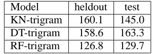
Model heldout test KN-trigram 160.1 145.0 DT-trigram 158.6 163.3 RF-trigram 126.8 129.7

Table 1: PPL for KN, DT, RF -trigram

can see from Table 1, DT-trigram obtained a slightly lower PPL than KN-trigram on heldout data, but was much worse on the test data. However, the RF-trigram performed much better on both heldout and

2

test data: our RF-trigram reduced the heldout data PPL from 160.1 to 126.8, or by 20.8%, and the test data PPL by 10.6%. Although we would expect im-provements from the DT-trigram on the heldout data since it is used to prune the fully grown DT, the ac-tual gain using a single DT is quite small (0.9%).

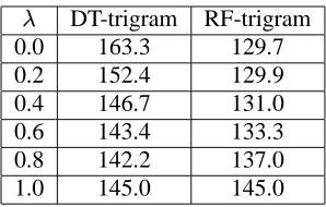
We also interpolated the DT-trigram and RF-trigram with the KN-RF-trigram at different levels of interpolation weight on the test data. It is inter-esting to see from Table 2 that interpolating KN-trigram with DT-KN-trigram results in a small improve-ment (1.9%) over the KN-trigram, when most of the interpolation weight is on KN-trigram (n

Z$ ). However, interpolating KN-trigram with

RF-trigram does not yield further improvements over RF-trigram by itself. Therefore, the RF modeling approach directly improves KN estimates by using randomized history clustering.

n DT-trigram RF-trigram

0.0 163.3 129.7 0.2 152.4 129.9 0.4 146.7 131.0 0.6 143.4 133.3 0.8 142.2 137.0 1.0 145.0 145.0

Table 2: Interpolating KN-trigram with DT,RF

-trigram for test data

4.2 Analysis

Our final model given by Equation 10 can be thought of as performing randomized history clus-tering in which each history is clustered into dif-ferent equivalence classes with equal probability. In order to analyze why this RF approach can improve the PPL on test data, we split the events (an event is a predicted word with its history) in test data into two categories: seen events and unseen events. For KN-trigram, seen events are those that appear in the training or heldout data at least once. For DT-trigram, a seen event is one whose predicted word is seen following the equivalence class of the history. For RF-trigram, we define seen events as those that are seen events in at least one DT among the random collection of DTs.

It can be seen in Table 3 that the DT-trigram re-duced the number of unseen events in the test data from 54.4% of the total events to 41.9%, but it in-creased the overall PPL. This is due to the fact that we used heldout data for pruning. On the other hand, the RF-trigram reduced the number of unseen events greatly: from 54.4% of the total events to only 8.3%. Although the PPL of remaining unseen

Model seen unseen

%total PPL %total PPL KN-trigram 45.6% 19.7 54.4% 773.1 DT-trigram 58.1% 26.2 41.9% 2069.7 RF-trigram 91.7% 75.6 8.3% 49814

Table 3: PPL of seen and unseen test events

events is much higher, the overall PPL is still im-proved. The randomized history clustering in the RF-trigram makes it possible to compute probabili-ties of most test data events without relying on back-off. Therefore, the RF-trigram can effectively in-crease the probability of those events that will oth-erwise be backoff to lower order statistics.

In order to reveal more about the cause of im-provements, we also compared the KN-trigram and RF-trigram on events that are seen in different num-ber of DTs. In Table 4, we splitted events into smaller groups according the the number of times they are seen among the 100 DTs. For the events

seen times %total KN-trigram RF-trigram

0 8.3% 37540 49814

1 3.0% 9146.2 10490

2 2.3% 5819.3 6161.4

3 1.9% 3317.6 3315.0

4 1.7% 2513.6 2451.2

5-9 6.1% 1243.6 1116.5 10-19 8.3% 456.0 363.5 20-29 5.7% 201.1 144.5 30-39 4.6% 123.9 83.0

40-49 4.0% 83.4 52.8

50-59 3.4% 63.5 36.3

60-69 2.5% 46.6 25.5

70-79 1.6% 40.5 20.6

80-89 0.7% 57.1 21.6

90-99 0.3% 130.8 39.9

100 45.7% 19.8 19.6

all 100% 145.0 129.7

Table 4: Test events analyzed by number of times seen in 100 DTs

proba-bility. This is also true for each DT. According to Equation 10, the more times an event is seen in the DTs, the more high probabilities it gets from the DTs, therefore, the higher the final aggregated probability is. In fact, we can see from Table 4 that the PPL starts to improve when the events are seen in 3 DTs. The RF-trigram effectively makes most of the events seen more than 3 times in the DTs, thus assigns them higher probabilities than the KN-trigram.

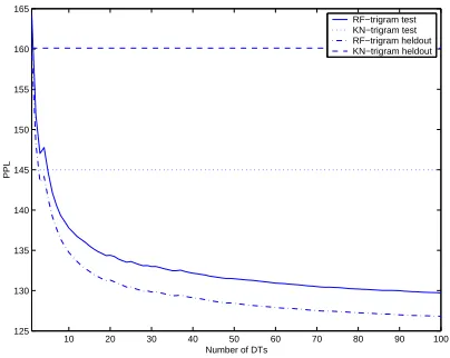
There is no theoretical basis for choosing the number of DTs needed for the RF model to work well. We chose to grow 100 DTs arbitrarily. In Fig-ure 1, we plot the PPL of the RF-trigram on held-out and test data as a function of number of DTs. It is clear that the PPL drops sharply at the begin-ning and tapers off quite quickly. It is also worth noting that for test data, the PPL of the RF-trigram with less than 10 DTs is already better than the KN-trigram.

10 20 30 40 50 60 70 80 90 100

125 130 135 140 145 150 155 160 165

Number of DTs

PPL

RF−trigram test KN−trigram test RF−trigram heldout KN−trigram heldout

Figure 1: Aggregating DTs in the RF-trigram

4.3 -best Re-scoring Results

To test our RF modeling approach in the context of speech recognition, we evaluated the models in the WSJ DARPA’93 HUB1 test setup. The size of the test set is 213 utterances, 3,446 words. The 20k words open vocabulary and baseline 3-gram model are the standard ones provided by NIST and LDC. The lattices and -best lists were generated using

the standard 3-gram model trained on 40M words of WSJ text. The -best size was at most 50 for

each utterance, and the average size was about 23. We trained KN-trigram and RF-trigram using 20M words and 40M words to see the effect of training data size. In both cases, RF-trigram was made of 100 randomly grown DTs and the global Bernoulli trial probability was set to 0.5. The results are re-ported in Table 5.

Model n

0.0 0.2 0.4 0.6 0.8 KN (20M) 14.0 13.6 13.3 13.2 13.1 RF (20M) 12.9 12.9 13.0 13.0 12.7

KN (40M) 13.0 - - -

-RF (40M) 12.4 12.7 12.7 12.7 12.7

Table 5: -best rescoring WER results

For the purpose of comparison, we interpolated all models with the KN-trigram built from 40M words at different levels of interpolation weight. However, it is the n =0.0 column (n is the weight

on the KN-trigram trained from 40M words) that is the most interesting. We can see that under both conditions the RF approach improved upon the reg-ular KN approach, for as much as 1.1% absolute when 20M words were used to build trigram mod-els. Standard -test3 shows that the improvements are significant at 0.001 and 0.05 level

re-spectively.

However, we notice that the improvement in WER using the trigram with 40M words is not as much as the trigram with 20M words. A possible reason is that with 40M words, the data sparseness problem is not as severe and the performance of the RF approach is limited. It could also be because our test set is too small. We need a much larger test set to investigate the effectiveness of our RF approach.

5 Conclusions and Future Work

We have developed a new RF approach for language modeling that can significantly improve upon the KN smoothing in both PPL and WER. The RF ap-proach results in a random history clustering which greatly reduces the number of unseen events com-pared to the KN smoothing, even though the same training data statistics are used. Therefore, this new approach can generalize well on unseen test data. Overall, we can achieve more than 10% PPL re-duction and 0.6-1.1% absolute WER rere-duction over the interpolated KN smoothing, without interpolat-ing with it.

Based on our experimental results, we think that the RF approach for language modeling is very promising. It will be very interesting to see how our approach performs in a longer history than the trigram. Since our current RF models uses KN smoothing exclusively in lower order probabilities,

3

For the*

it may not be adequate when we apply it to higher order -gram models. One possible solution is to

use RF models for lower order probabilities as well. Higher order RFs will be grown based on lower or-der RFs which can be recursively grown.

Another interesting application of our new ap-proach is parser based language models where rich syntactic information is available (Chelba and Je-linek, 2000; Charniak, 2001; Roark, 2001; Xu et al., 2002). When we use RFs for those models, there are potentially many different syntactic ques-tions at each node split. For example, there can be questions such as “Is there a Noun Phrase or Noun among the previous exposed heads?”, etc. Such

kinds of questions can be encoded and included in the history. Since the length of the history could be very large, a better smoothing method would be very useful. Composite questions in the form of py-lons (Bahl et al., 1989) can also be used.

As we mentioned at the end of Section 3.2, ran-dom samples of the training data can also be used for DT growing and has been proven to be useful for classification problems (Amit and Geman, 1997; Breiman, 2001; Ho, 1998). Randomly sampled data can be used to grow DTs in a deterministic way to construct RFs. We can also construct an RF for each random data sample and then aggregate across RFs. Our RF approach was developed for language modeling, but the underlying methodology is quite general. Any -gram type of modeling should be

able to take advantage of the power of RFs. For ex-ample, RFs could also be useful for POS tagging, parsing, named entity recognition and other tasks in natural language processing.

References

Y. Amit and D. Geman. 1997. Shape quantization and recognition with randomized trees. Neural Computation, (9):1545–1588.

L. Bahl, P. Brown, P. de Souza, and R. Mercer. 1989. A tree-based statistical language model for natural language speech recognition. In IEEE Transactions on Acoustics, Speech and Signal Processing, volume 37, pages 1001–1008, July. Yoshua Bengio, Rejean Ducharme, and Pascal

Vin-cent. 2001. A neural probabilistic language model. In Advances in Neural Information Pro-cessing Systems.

L. Breiman, J.H. Friedman, R.A. Olshen, and C.J. Stone, 1984. Classification and Regression Trees. Chapman and Hall, New York.

Leo Breiman. 2001. Random forests. Technical re-port, Statistics Department, University of Califor-nia, Berkeley, Berkeley, CA.

Eugene Charniak. 2001. Immediate-head pars-ing for language models. In Proceedpars-ings of the 39th Annual Meeting and 10th Conference of the European Chapter of ACL, pages 116–123, Toulouse, France, July.

Ciprian Chelba and Frederick Jelinek. 2000. Struc-tured language modeling. Computer Speech and Language, 14(4):283–332, October.

Stanley F. Chen and Joshua Goodman. 1998. An empirical study of smoothing techniques for lan-guage modeling. Technical Report TR-10-98, Computer Science Group, Harvard University, Cambridge, Massachusetts.

P.A. Chou. 1991. Optimal partitioning for classifi-cation and regression trees. IEEE TRans. on Pat-tern Analysis and Machine Intelligence, 13:340– 354.

T.K. Ho. 1998. The random subspace method for constructing decision forests. IEEE Trans. on Pattern Analysis and Machine Intelligence, 20(8):832–844.

Frederick Jelinek, 1997. Statistical Methods for Speech Recognition. MIT Press.

Reinhard Kneser and Hermann Ney. 1995. Im-proved backing-off for m-gram language model-ing. In Proceedings of the ICASSP, volume 1, pages 181–184.

S. Martin, J. Liermann, and H. Ney. 1998. Algo-rithms for bigram and trigram word clustering. Speech Communication, 24:19–37.

Gerasimos Potamianos and Frederick Jelinek. 1998. A study of n-gram and decision tree letter language modeling methods. Speech Communi-cation, 24(3):171–192.

Brian Roark. 2001. Robust Probabilistic Predic-tive Syntactic Processing: Motivations, Models and Applications. Ph.D. thesis, Brown Univer-sity, Providence, RI.

Holger Schwenk and Jean-Luc Gauvain. 2002. connectionist language modeling for large vocab-ulary continuous speech recognition. In Proceed-ings of the ICASSP, pages 765–768, Orlando, Florida, May.

Andreas Stolcke. 2002. Srilm – an extensible lan-guage modeling toolkit. In Proc. Intl. Conf. on Spoken Language Processing, pages 901–904, Denver, CO.