Engineering Education: Computer Aided Engineering with MATLAB; Discrete Wavelet Transform as a Case Study

Engineering Education: Computer-Aided Engineering

with MATLAB; Discrete Wavelet Transform as a Case

Study

Abdul Rasak Zubair

Electrical/Electronic Engineering Department University of Ibadan, Ibadan, Nigeria

Yusuf Kola Ahmed

Biomedical Engineering Department

University of Ilorin, Ilorin, Nigeria

M.Sc. Program: Electrical/Electronic Engineering Dept., University of Ibadan, Ibadan, Nigeria

ABSTRACT

Engineering education is to move engineering students along the progressive path from being novices toward becoming experts in design, problem-solving and application of knowledge. Engineering problem may require more computations than is possible by hand. Computer-aided engineering is the process of solving engineering problems with the aid of computer software. Engineering Lecturers need to help engineering students to develop expertise in Computer-aided engineering with examples. The development of Discrete Wavelet Transformation is used as a case study. A wavelet is a small wave whose energy is concentrated in time. Wavelets applications include signal processing, noise filtering, image processing, and document analysis. Among wavelet families, Haar wavelet is selected. Scientific representations of the problem and a logical plan of attacking the problem are presented. Necessary equations are derived. A modular approach to programming is demonstrated. A complex problem is broken down into simple tasks and steps which are coded into simple short MATLAB programs. A program calls another program to execute some specific tasks. Programs are checked against possible errors using a situation where the answers are known. Discrete wavelet transformation and inverse discrete wavelet transformation for 1D, 2D, and 3D discrete-time signals have been implemented. 2D gray level images and 3D color images are also considered. The use of similar examples is recommended for Engineering Lecturers.

General Terms

Digital Signal Processing, Digital Image Processing, Algorithm Development.

Keywords

Engineering Education, Problem-solving, Computer-aided engineering, MATLAB, Discrete Wavelet transformation.

1.

INTRODUCTION

The objective of engineering education is to move engineering students along the progressive path from being novices toward becoming experts in design, problem-solving and application of knowledge [1]. The Engineering Lecturers have the duty to lead the engineering students from what they know to what they do not know. Studies have revealed that students have misunderstandings with regards to a range of concepts [2], [3], [4]. Improving the understanding and technical know-how of students are tasks that should be accomplished by Lecturers.

Problem-solving is required whenever there is a goal to reach and attainment of that goal is not possible either by direct action or by retrieving a sequence of previously learned steps from memory [4], [5]. During problem-solving, the path to the intended goal is uncertain.

Some of the problems to be solved may be well-defined or ill-defined [7]. Most problems in class are well ill-defined; initial conditions, goal, means for generating and evaluating the solution, and the constraints on the solution are specified. For the ill-defined problems, students need to define some of the problems’ components on their own [7]. Regular practice is important [8]. Practice makes perfect.

Formulation of scientific representations of the problem to be solved in the form of pictures, diagrams, graphs, maps, models, and simulations facilitates problem-solving. A problem representation is the model of the problem constructed by the solver to summarize his/her understanding of the problem. This model may include the elements in the problem, the inter-relationship of the elements, the goals and the types of operations that can be performed on the elements, and any constraints on the solution process.

Yildirim, Shuman and Besterfield-Sacre in [9] recommend that the expert should guide the novice toward success. The expert needs to point out the strengths and weaknesses of the novice’s product or performance. Teamwork among students to solve open-ended, real-world problems can also improve students’ problem-solving skills.

Solution to an engineering problem may require more computations than is possible by hand. A digital computer is, therefore, an essential tool in solving engineering problems [10], [11], [12]. Engineering students need to be familiar with Computer-aided engineering which is the process of solving engineering problems with the aid of computer software.

MATLAB computer programming system is a problem-solving tool for scientists and engineers [13], [14]. It has a teach-yourself feature. MATLAB is based on the mathematical concept of a matrix. Every variable X is a matrix of order m-by-n; m rows and n columns. A matrix is a rectangular array. A vector is a list or a matrix with 1 column or with 1 row. A constant k is a scalar and it’s a 1-by-1 matrix. Regarding all variables as matrices is an official MATLAB mindset [13].

exponentiation, and all usual mathematical functions like Sin, Cos, Log, exp, square and square root just to mention a few. MATLAB can also handle logical operations. Values can be assigned to variables and arithmetic operations can be done on variables. It has numerous functions and commands. MATLAB can plot graphs. MATLAB can solve simultaneous equations. It has a very useful ‘help’ system.

MATLAB has program repetition feature which enables iteration. A set of instructions is executed a predefined number of times using the ‘for’ or the ‘while’ operator. The ‘break’ operator can terminate the repetition when a condition is met. The ‘continue’ operator is also used in the repetition feature to achieve some tasks.

Decision making is another important feature of MATLAB which uses logical ‘if else statement’. A set S1 of instructions is executed if a logical statement is true otherwise another set S2 of instructions is executed. More than two sets of instructions can be accommodated by including one or more ‘elseif’ operators.

Solving a problem requires developing a logical plan of attack to solve the problem. The Engineer needs to understand the problem, develop scientific representations of the problem, and develop correct systematic steps for solving the problem. A clear understanding of the arithmetic and logical operations involved in the solution is essential. The correctness of these steps needs to be critically and carefully studied. These steps need to be further broken down into sub-steps that MATLAB can handle. Wrong steps will give the wrong solution. Repetitive or iterative nature of some of the steps should be carefully handled. If garbage goes in, garbage would come out. There will always be an answer; the answer may be correct or wrong. It’s even worse if the Engineer does not know the answer is wrong or why the answer is wrong [13].

Checking algorithm against possible errors is essential. One error detecting method is running the program for special situations where the Engineer knows the answers [13]. For example, if the problem is the multiplication of two matrices, manually multiply a 3-by-3 matrix by a 3-by-2 matrix and compare the results with the output of the program. Manual calculation of a small scale version of the problem is a way of validating the output of a program. If the output of the program does not tally with the known answer, such program requires checking against possible arithmetic, logical and language errors.

An algorithm is a systematic logical procedure for solving a problem. The algorithm is represented by a structured plan. The algorithm is then coded into a MATLAB program often referred to as M-file; the sub-steps are faithfully translated into MATLAB language. The translation must be correct and faithful otherwise the correctness of the answer is compromised.

A modular approach to programming is recommended. Troubleshooting, debugging and testing the program becomes easier as modules can be debugged or tested module by module. A complex problem can be solved with several subprograms. A MATLAB program (main program) can call and execute other programs (subprograms) within it. A subprogram is a complete program on its own and can be executed if called within another program.

In the beginning, an Engineer may find it difficult. Over time, an Engineer builds experience in algorithm development and such development becomes easy or automatic. In this work,

the development of Discrete Wavelet Transformation is taken as a case study.

A wavelet is defined as a small wave whose energy is concentrated in time [15], [16], [17], [18], [19]. Wavelets applications include signal processing, noise filtering, image processing, image compression, image recognition, document analysis, and feature extraction [18], [20], [21], [22]. Haar wavelet is selected. There are other wavelet families such as Daubechies (Db), Sinc, Gaussian and Mexican Hat as illustrated in Fig. 1 [15].

2.

DISCRETE WAVELET TRANSFORM

2.1

Review of One-Dimensional DWT

Given a discrete-time signal X which is an N-by-1 matrix. It is required to determine Y, the one-dimensional discrete wavelet transform (1D DWT) of X at Lmth decomposition level. For

example, suppose X is given as in Eqn. (1).



X





















































8

6

7

4

0

1

3

2

(1)

N is 8 in this example. Y is first set equal to X, YX. Y is broken into y1 and y2 as shown in Fig. 2. y1 is set equal to Y

as y2 is empty. y1 and y2 are used to multiply the wavelet

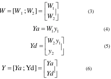
transformation matrix W and an Identity Matrix I respectively for the first decomposition level as illustrated in Fig. 2 and as described by Eqn. (2). The wavelet transformation matrix W is given by Eqn. (3). W1 and W2 are the approximate and

detail wavelet transformation matrices respectively; they are regarded as low pass (lp) filter and high pass (hp) filter respectively. Y is also decomposed into two parts as described by Eqns. (4), (5), (6); the approximate part Ya which contains the low-frequency information of the signal and the details part Yd which contains the high-frequency information of the signal.

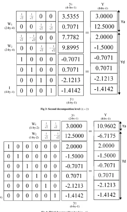
The output Y at the end of the first decomposition level is feedback and packaged as y1 and y2 which are used to

multiply the wavelet transformation matrix W and an Identity Matrix I respectively for the second decomposition level as shown in Fig. 3. The output Y at the end of the second decomposition level is feedback and packaged as y1 and y2

which are used to multiply the wavelet transformation matrix W and an Identity Matrix I respectively for the third decomposition level as shown in Fig. 4. At the end of every decomposition level, Y is decomposed into the approximate part (Ya) and the details part (Yd) as described by Eqns. (4), (5), (6).

Y



_

[image:3.595.82.521.71.551.2]

Fig 1: Some wavelet families

Fig 2: First decomposition level (L1)





[

W

₁

;

W

₂

]

W

_











2 1

W

W

(3)

Ya



W

₁

y

₁ (4)















2 1 2

y

y

W

Yd

(5)





[

Ya

;

Yd

]

Y

_











Yd

Ya

(6)

Observations on the relationship between the dimensions of X, Y, W1, W2, y1, y2, Ya and Yd on one hand and the

decomposition level (L) and the number of elements (N) in X on the other hand are summarized in Table 1. Both X and Y are N-by-1. Both W1 and W2 are r-by-c. r is usually half of c.

y1 is c-by-1, y2 is (N-c)-by-1, Ya is r-by-1, and Yd is

(N-r)-by-1. r and c are related to N and L as indicated in Table 1 and Eqns. (7) and (8). These equations are deduced from the trends in Table 1. W1 and W2 are concatenated to give W as in

Eqn. (3) which is a MATLAB statement. Similarly, Wy1 and

Iy2 are concatenated to give Y as in Eqn. (2).

L

N

r

2



(7)

₁

2





N

_L

[image:3.595.86.280.562.700.2]

[image:4.595.85.503.66.761.2] [image:4.595.99.499.70.419.2]

Fig 3: Second decomposition level (L2)

[image:5.595.56.541.88.302.2]

Table 1. Observations on dimensions of variables Decomposition

Level

W1 W2 W I y1 y2 Ya Yd

L=1 4-by-8 4-by-8 8-by-8 - 8-by-1 0-by-1 4-by-1 4-by-1

L=2 2-by-4 2-by-4 4-by-4 4-by-4 4-by-1 4-by-1 2-by-1 6-by-1

L=3 1-by-2 1-by-2 2-by-2 6-by-6 2-by-1 6-by-1 1-by-1 7-by-1

Generally for L and N r-by-c L

N

r

2



1

2





N

_L

c

r-by-c L

N

r

2



1

2





N

_L

c

c-by-c

1

2





N

_L

c

(N-c)-by-(N-c) c-by-1

1

2





N

_L

c

(N-c)-by-1

1

2





N

_L

c

r-by-1 L

N

r

2



(N-r)-by-1 L

N

r

2



X is N-by-1; (N8 in this example.)



W

_











2 1

W

W

;

Y















2 1

Iy

Wy

;

Y















Yd

Ya

; Y is also N-by-1

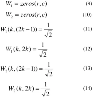
W1 and W2 are the approximate and detail wavelet

transformation matrices respectively. Most of the elements of W1 andW2 are zeroes. Few of the elements of W1 andW2 are

2 1 or

2 1

 . Eqns. (9) and (10) set all elements of W1 and

W2 to zero. A careful review of W1 in Figs. 4, 5 and 6 shows

that on the kth row, the (2k)th column and the (2k-1)th column are both

2

1 . A careful review of W2 in Figs. 4, 5 and 6

shows that on the kth row, the (2k)th column and the (2k-1)th column are

2 1

 and 2

1 respectively. Therefore, Eqns.

(11), (12), (13) and (14) set specific elements of W1 andW2 to

2 1

 or 2

1 as appropriate. The solution is repetitive for

each decomposition level L=1, 2, 3, up to the specified level L=Lm.

W

1



zeros

(

r

,

c

)

(9)

W

2



zeros

(

r

,

c

)

(10)

2

1

))

1

2

(

,

(

1

k

k





W

(11)

2

1

)

2

,

(

1

k

k



W

(12)

2

1

))

1

2

(

,

(

2

k

k





W

(13)

2

1

)

2

,

(

2

k

k



W

(14)

2.2

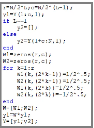
Basic Haar Wavelet Program

Given the Y at the end of last decomposition level, it is required to determine r, c, y1, y2, W1, and W2 using Eqns. (7)

to (14) and update Y using Eqns. (2) and (3) for the next decomposition level (L). A program is developed to carry out this task. This program is named haarbasic. Its flow chart and MATLAB codes are presented in Figs. 5 and 6 respectively.

The inverse transform program INVhaarbasic is presented in Fig. 7. INVhaarbasic is similar to haarbasic except for the fact that Eqn. (2) is replaced by Eqn. (15).

[image:5.595.310.550.358.745.2]



Y

_











 2 1 1

Iy

y

W

_













 2 1 1

y

y

W

(15)

[image:5.595.122.280.516.680.2]

[image:6.595.91.247.72.284.2] [image:6.595.331.519.159.508.2]

Fig 6: haarbasic program for decomposition level L

Fig 7: INVhaarbasic program for decomposition level L

2.3

One-Dimensional DWT Program

2.3.1

Column Signal

Given an input column signal X (N-by-M) where M1, it is required to determine Y, the one-dimensional discrete wavelet transform (1D DWT) of X at Lmth decomposition level.

Initialize Y as YX. Starting with L1, call the haarbasic program, increase L and repeat the call of the haarbasic program up to L=Lm as illustrated in the flowchart of Fig. 8. Y

obtained at the end of LL_m is the required 1D DWT of X. The flow chart of Fig. 8 is coded into a MATLAB program named dwt1Dc and presented in Fig. 9. The inverse transform program INVdwt1Dc presented in Fig. 10 is similar to dwt1Dc except that L decreases from Lm to 1 in INVdwt1Dc whereas L

increases from 1 to Lm in dwt1Dc.

2.3.2

Row Signal

Given an input row signal X (M-by-N) where M1, It is required to determine Y, the one-dimensional discrete wavelet transform (1D DWT) of X at Lmth decomposition level.

Change X from being a row signal into a column signal. Call dwt1Dc program. Change the final output Y from being a column signal to a row signal. The new program is named dwt1Dr and is presented in Fig 11. The inverse transform program INVdwt1Dr presented in Fig. 12 is similar to dwt1Dr. Change Y from being a row signal into a column signal. Call INVdwt1Dc program. Change the final output X from being a column signal to a row signal.

Fig 8: Flow chart of the dwt1Dc program for a column 1D signal

Fig 9: dwt1Dc program for a column 1D signal

[image:6.595.88.250.311.526.2]

Fig 11: dwt1Dr program for a row 1D signal

Fig 12: INVdwt1Dr program for a row 1D signal

2.4

Two-Dimensional DWT Program

Given a two-dimensional signal or gray level image XX (NN-by-MM), It is required to determine YY, the two-dimensional discrete wavelet transform (2D DWT) of XX at LLmth

decomposition level. Initialize YY as YYXX. If XX is a gray level image, XX should be converted from uint8 format to double format before applying it as input. The output YY should be converted from double format to uint8 format before displaying it as an image.

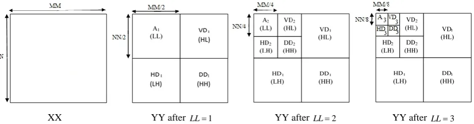
The 2D DWT of a signal or image can be partitioned into four regions or components namely: Approximation (A), Horizontal details (HD), Vertical details (VD), and Diagonal details (DD) as illustrated in Fig. 13. A, HD, VD, and DD are the Low/Low (LL), Low/High (LH), High/Low (HL) and the High/High (HH) frequency components of the signal respectively. At the next decomposition level, the Approximation part is further divided into another set of A, HD, VD, and DD as shown in Fig. 13.

1D DWT and inverse 1D DWT programs are required here as subprograms. The outputs of these subprograms constitute intermediate results in 2D DWT program and such outputs may be disabled from being published with ‘;’ .

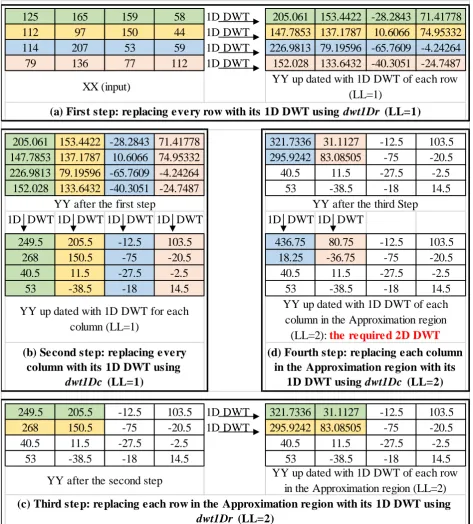
Starting with the decomposition level LL1, work on the entire YY (NN-by-MM). Take the first row in YY as X and call dwt1Dr with Lm 1. Update YY by replacing the first row of YY with the Y obtained from dwt1Dr. Repeat for all the rows in YY. This is illustrated in Fig. 14 (a) tagged as the first step. Take the first column in the updated YY as X and call dwt1Dc with Lm1. Update YY by replacing the first

column of YY with the Y obtained from dwt1Dc. Repeat for all the columns in YY as illustrated in Fig. 14 (b) tagged as the second step. The YY at the end of the second step is the two-dimensional discrete wavelet transform (2D DWT) for

1



LL .

For LLLL, select the Approximation component which is the NN/LL-by-MM/LL top-left-portion of the updated YY and repeat the procedure above. The remaining portions of YY remain unchanged. For LL2, 2-by-2 top-left-portion of YY is taken and the procedure is repeated as illustrated in Fig. 14 (c) and (d) tagged third and fourth step respectively. Increase LL from 1 up to LLm. In Fig. 14, the operations

stopped at LL2 because LLm is given as 2. A program

named as dwt2D is developed and presented in Fig. 15. MATLAB code ‘clear’ is introduced in this program during test running when an error was observed. This code deletes a variable in the workspace or memory. For example, when LL changed from 1 to 2 in Fig. 14, the dimension of both X and Y changed from 1-by-4 to 1-by-2. If X and Y are not cleared before the change in LL, X and Y will remain 1-by-4 after the change in LL instead of 1-by-2 which actually led to an error during test running.

The steps for the inverse two-dimensional discrete wavelet transform program INVdwt2D of Fig. 16 are similar. In dwt2d, LL increases from 1 up to LLm and rows are operated before

columns. In INVdwt2D, LL decreases from LLm down to 1

and columns are operated before rows.

2.5

Three-Dimensional DWT Program

Given a three-dimensional signal or color image x (NN-by-MM-by-3), It is required to determine y, the three-dimensional discrete wavelet transform (3D DWT) of y at LLmth decomposition level. This is accomplished by simply

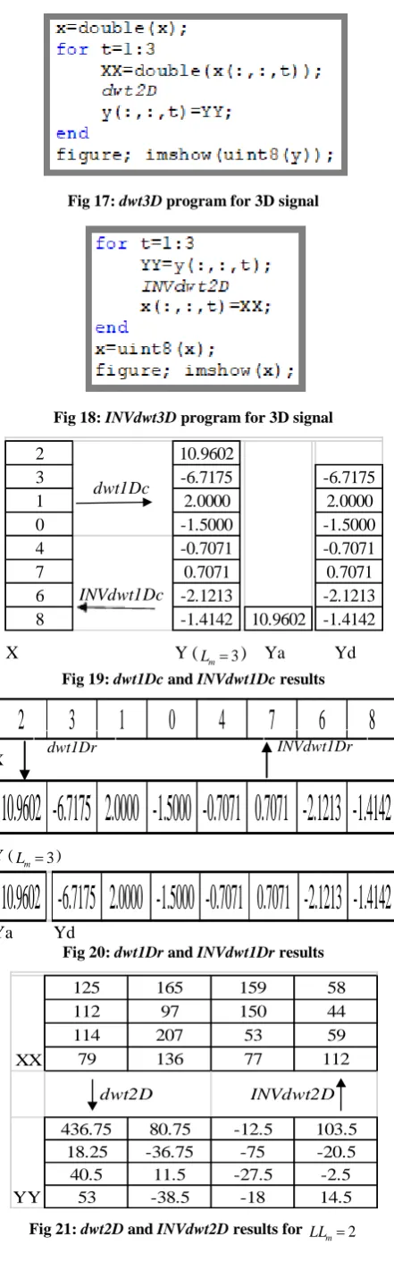
finding the 2D DWT of each of the red, green and blue components of x. dwt2D is executed three times as indicated in the dwt3D program of Fig. 17.

The first line in Fig. 17 converts the color image from the uint8 format to the double format. The output 3D DWT (y) should not be converted from the double format to the uint8 format otherwise original x will not be recoverable from y via the INVdwt3D program of Fig. 18 which is the inverse 3D DWT program. The last line in Fig. 17 shows the image of uint8 version of y on a fresh figure. The second to the last line in Fig. 18 converts the inverse 3D DWT from the double format back to the uint8 format.

[image:7.595.66.545.568.694.2]

XX YY after LL1 YY after LL2 YY after LL3

[image:8.595.62.536.72.597.2]

Fig 14: Illustration of 2D DWT for a 4-by-4 input at decomposition level LLm2

3.

RESULTS AND DISCUSSIONS

Validation tests for the 1D and 2D DWT and inverse DWT programs were carried out for situations when the results are known. As shown in Figs. 19, 20, 21 and 22, the outputs of the 1D and 2D DWT and inverse DWT programs are found to be valid. When the output of the DWT program is supplied as input to the corresponding inverse DWT program, the output of the inverse DWT program is found in all cases to be equal to the initial input to the DWT program as illustrated in Figs. 19, 20, 21 and 22.

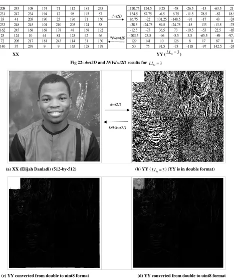
2D DWT and inverse 2D DWT programs are also tested with a gray level image. The results are presented in Figs. 23 (a)

and (b). YY in Fig. 23(b) is in double format which gives Fig. 23(c) when converted to uint8 format. Application of image enhancement on the Approximation component gives Fig. 23(d). The image enhancement is accomplished by replacing each element e of the approximation component with p

e where p0.7. The approximation component is thus a version of the original input image but with reduced size (dimension). The VD, HD, and DD give the vertical, horizontal and diagonal edges (details) of the input image.

3D DWT and inverse 3D DWT programs are tested with a color image. The results are presented in Figs. 24 (a) and (b). y in Fig. 24(b) is in the double format which gives Fig. 24(c)

125

165

159

58

205.061

153.4422 -28.2843 71.41778

112

97

150

44

147.7853 137.1787

10.6066

74.95332

114

207

53

59

226.9813 79.19596 -65.7609 -4.24264

79

136

77

112

152.028

133.6432 -40.3051 -24.7487

205.061

153.4422 -28.2843 71.41778

321.7336

31.1127

-12.5

103.5

147.7853 137.1787

10.6066

74.95332

295.9242 83.08505

-75

-20.5

226.9813 79.19596 -65.7609 -4.24264

40.5

11.5

-27.5

-2.5

152.028

133.6432 -40.3051 -24.7487

53

-38.5

-18

14.5

1D DWT 1D DWT 1D DWT 1D DWT

1D DWT 1D DWT

249.5

205.5

-12.5

103.5

436.75

80.75

-12.5

103.5

268

150.5

-75

-20.5

18.25

-36.75

-75

-20.5

40.5

11.5

-27.5

-2.5

40.5

11.5

-27.5

-2.5

53

-38.5

-18

14.5

53

-38.5

-18

14.5

249.5

205.5

-12.5

103.5

321.7336

31.1127

-12.5

103.5

268

150.5

-75

-20.5

295.9242 83.08505

-75

-20.5

40.5

11.5

-27.5

-2.5

40.5

11.5

-27.5

-2.5

53

-38.5

-18

14.5

53

-38.5

-18

14.5

(c) Third step: replacing each row in the Approximation region with its 1D DWT using

dwt1Dr

(LL=2)

YY after the third Step

(d) Fourth step: replacing each column

in the Approximation region with its

1D DWT using

dwt1Dc

(LL=2)

1D DWT

1D DWT

YY after the second step

YY up dated with 1D DWT of each row

in the Approximation region (LL=2)

1D DWT

1D DWT

1D DWT

(a) First step: replacing every row with its 1D DWT using

dwt1Dr

(LL=1)

XX (input)

YY up dated with 1D DWT of each row

(LL=1)

YY after the first step

YY up dated with 1D DWT for each

column (LL=1)

YY up dated with 1D DWT of each

column in the Approximation region

(LL=2):

the required 2D DWT

(b) Second step: replacing every

column with its 1D DWT using

dwt1Dc

(LL=1)

when converted to the uint8 format. Application of image enhancement on the Approximation component gives Fig. 24(d). The image enhancement is accomplished by replacing each element e of the approximation component with p

[image:9.595.320.541.67.774.2]

e where p0.8.

[image:9.595.107.538.88.755.2]

Fig 15: dwt2D program for 2D signal

[image:9.595.89.245.113.707.2]

Fig 16: INVdwt2D program for 2D signal

Fig 17: dwt3D program for 3D signal

Fig 18: INVdwt3D program for 3D signal

X Y ( _3 m

[image:9.595.93.245.141.441.2]

L ) Ya Yd

Fig 19: dwt1Dc and INVdwt1Dc results

X

Y (L_m3)

Ya Yd

Fig 20: dwt1Dr and INVdwt1Dr results

Fig 21: dwt2D and INVdwt2D resultsfor LL_m2

2 10.9602

3 -6.7175 -6.7175

1 2.0000 2.0000

0 -1.5000 -1.5000

4 -0.7071 -0.7071

7 0.7071 0.7071

6 -2.1213 -2.1213

8 -1.4142 10.9602 -1.4142 dwt1Dc

INVdwt1Dc

2

3

1

0

4

7

6

8

10.9602 -6.7175 2.0000 -1.5000 -0.7071 0.7071 -2.1213 -1.4142

10.9602 -6.7175 2.0000 -1.5000 -0.7071 0.7071 -2.1213 -1.4142

125 165 159 58

112 97 150 44

114 207 53 59

79 136 77 112

436.75 80.75 -12.5 103.5 18.25 -36.75 -75 -20.5 40.5 11.5 -27.5 -2.5

53 -38.5 -18 14.5

dwt2D INVdwt2D

XX

YY

[image:9.595.90.244.423.705.2]

[image:10.595.65.533.64.620.2]

XX YY (LLm3₎ Fig 22: dwt2D and INVdwt2D resultsfor LLm3

(a) XX (Elijah Danladi) (512-by-512) (b) YY ( _3 m

LL ) (YY is in double format)

(c) YY converted from double to uint8 format (d) YY converted from double to uint8 format and the approximation component is enhanced

Fig 23: dwt2D and INVdwt2D resultsfor LL_m3 The approximation component is thus a version of the original

input image but with reduced size. The VD, HD, and DD give the vertical, horizontal and diagonal edges (details) of the input image.

4.

CONCLUSIONS

Development of a logical plan of attack in solving a problem has been demonstrated. Scientific representations of the problem in the form of diagrams were presented. Arithmetic

and logical relationships between the input, output and intermediate variables in the form of mathematical equations were derived. Simple relevant tools of MATLAB were used in developing the programs for solving the problem. Programs were developed in modules. A program may call another program for some specific tasks. A complex problem is solved by simple programs instead of one long complex program. Simple short programs are easier to develop and debug.

208 245 108 174 71 112 181 245 1120.75 124.5 9.25 -58 -26.5 -13 -63.5 21

231 247 234 194 12 98 193 87 134.5 87.75 -6.5 6.75 -11.5 78.5 -82 18.5

33 41 203 190 25 196 71 150 86.75 -22 101.25 -148.5 -91 -17 43 -24

233 248 245 101 210 203 174 58 -38.5 -24.75 89.5 -24.75 -15 133 -13.5 -75

162 245 168 168 178 48 168 192 -12.5 -73 36.5 73 -10.5 -53 22.5 -85

25 124 10 44 81 125 42 66 -203.5 23.5 -96 -5.5 3.5 -65.5 -89 -97.5

72 205 217 181 243 114 31 130 129 141 10 126 8 17 87 0

140 37 239 9 9 165 128 179 50 75 91.5 -73 -118 -97 142.5 -24

INVdwt2D dwt2D

dwt2D

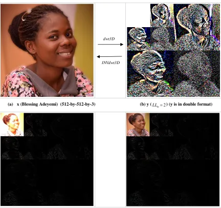
(a) x (Blessing Adeyemi) (512-by-512-by-3) (b) y (LLm2) (y is in double format)

(c) y converted from double to uint8 format (d) y converted from double to uint8 format and

[image:11.595.82.515.67.473.2]

the approximation component enhanced Fig 24: dwt3D and INVdwt3D resultsfor _2

m

LL Programs are validated with situations where the answers are

known. Discrete wavelet transformation and inverse discrete wavelet transformation have been demystified. Discrete wavelet transformation and inverse discrete wavelet transformation for 1D, 2D, and 3D discrete-time signals in general and gray level images and color images in particular have been implemented and can be applied in Discrete Signal Processing and Digital Image Processing. The use of similar examples is recommended for Engineering Lecturers for transforming Engineering students from novices to experts vis-a-vis computer-aided engineering and problem-solving.

5.

REFERENCES

[1] National Research Council, 2012. “Discipline-Based Education Research: Understanding and Improving Learning in Undergraduate Science and Engineering” Singer, S. R., Nielsen, N. R. and H. A. Schweingruber, H. A.Editors. Committee on the Status, Contributions, and Future Directions of Discipline-Based Education Research. Board on Science Education, Division of Behavioral and Social Sciences and Education. Washington, DC: The National Academies Press.

[2] Docktor, J. L., and Mestre, J. P. 2011. “A synthesis of discipline-based education research in physics”, Paper presented at the Second Committee Meeting on the Status, Contributions, and Future Directions of Discipline-Based Education Research. Available: http://www7.nationalacademies.org/bose/DBER_Dockto r_October_Paper.pdf.

[3] Svinicki, M. 2011. “Synthesis of the research on teaching and learning in engineering since the implementation of ABET engineering criteria 2000”, Paper presented at the Second Committee Meeting on the Status, Contributions, and Future Directions of Discipline-Based Education

Research. Available:

http://www7.nationalacademies.org/bose/DBER_Svinick i_October_Paper.pdf.

[4] Bassok, M. and Novick, L. R. 2012. “Problem solving”, In Holyoak, K. J. and Morrison, R. G. (Eds.), Oxford handbook of thinking and reasoning, 413-432. New York: Oxford University Press.

[5] Martinez, M. E. 2010. Learning and cognition: The design of the mind. Upper Saddle River, NJ: Merrill.

dwt3D

[6] Hsu, L., Brewe, E., Foster, T. M., and Harper, K. A. 2004. “Resource letter RPS-1: Research in problem solving”, American Journal of Physics, 72(9), 1147-1156.

[7] Whitson, L., Bretz, S. L., and Towns, M. H. 2008. “Characterizing the level of inquiry in the undergraduate laboratory”. Journal of College Science Teaching, 37(7), 52-58.

[8] Ericsson, K. A., Krampe, R. Th., and Tesch-Römer, C. 1993. “The role of deliberate practice in the acquisition of expert performance”. Psychological Review, 100(3), 363-406.

[9] Yildirim, T., Shuman, L., and Besterfield-Sacre, M. 2010. “Model-eliciting activities: Assessing engineering student problem solving and skill integration processes”, International Journal of Engineering Education, 26(4), 831-845.

[10]Zubair A. R. 2009. “Numerical Integration Based Analysis of Pulse Width Modulated Voltage Source Inverter”, In A. Gyasi-Agyei and T. Ogunfunmi (Eds.). Adaptive Science and Technology: Proceedings of the 2nd IEEE International Conference on Adaptive Science and Technology (ICAST). 14-16 December, 2009.

Accra, 301–307. Available at

https://ieeexplore.ieee.org/document/5409707.

[11]Zubair A. R. and Olatunbosun A. 2014. “Arithmetic and Logical Models of Transmission Line Stranded Conductors for Voltage and Voltage-Drop Analysis”, International Journal of Innovation and Scientific Research, 8(2), 200-209.

[12]Zubair A. R. and Olatunbosun A. 2014. “Computer Aided Root-Locus Numerical Technique”, Nigerian Journal of Technology, 33(1), 1-13.

[13]Hahn B. and Valentine D. T. 2007. Essential MATLAB for Engineers and Scientists. Burlington: Elsevier.

[14] MathWorks (Matlab). 2018. ‘‘Documentation for MathWorks products’’ Available: https://ch.mathworks.com/help/index.html.

[15] Soman, K. P. 2010. Insight into wavelets: From theory to practice. PHI Learning Pvt. Ltd, 45-237.

[16] Mallat, S. 2008. A wavelet tour of signal processing: the sparse way. Academic press, 80-336.

[17] Burrus, C. S., Gopinath, R. A., Guo, H., Odegard, J. E. and Selesnick, I. W. 1998. Introduction to wavelets and wavelet transforms: a primer. New Jersey, Prentice hall, 1, 7-111.

[18] Donoho, D. L. and Johnstone, I. M. 1994. “Ideal denoising in an orthonormal basis chosen from a library of bases”. Comptes Rendus de l’Académie Des Sciences. Série I, Mathématique, 319(12), 1317–1322.

[19] Van Fleet, P. J. 2011. Discrete wavelet transformations: An elementary approach with applications. John Wiley & Sons, 157-346.

[20] Hongqiao L. and Shengqian W. 2009. "A New Image Denoising Method Using Wavelet Transform", International Forum on Information Technology and Applications (IFITA), Chengdu, 111-114.

[21] Mithun, V. K., Pandey, P., Sebastian, P. C., Mishra, T. P. 2011. “A wavelet based technique for suppression of EMG noise and motion artifact in ambulatory ECG”, Engineering in Medicine and Biology Society, EMBC, 2011 Annual International Conference of the IEEE, 7087–7090.