A Study on Numerical Solution of Black Scholes Model

(1)

ISSN Online: 2162-2442 ISSN Print: 2162-2434

DOI: 10.4236/jmf.2018.82024 May 18, 2018 372 Journal of Mathematical Finance

A Study on Numerical Solution

of Black-Scholes Model

Md. Nurul Anwar

1,2*

, Laek Sazzad Andallah

1

1_{Department of Mathematics, Jahangirnagar University, Savar, Dhaka, Bangladesh}

2_{Department of Natural Science, BGMEA University of Fashion & Technology, Dhaka, Bangladesh}

Abstract

In the history of option pricing, Black-Scholes model is one of the most sig-nificant models. In this article, the main concern is the numerical solution of the Black-Scholes model (a.k.a. Black/Scholes/Merton) for the European call option in a different way. The model is described and an explicit difference scheme was used for the numerical approximation. The stability condition of the scheme is established through convex combination. A different way was used to obtain the numerical value of the model. Estimation of the relative er-ror was calculated in L1-norm in order to test the accuracy of the scheme. Fi-nally, a comparison of the numerical outcomes with the value obtained by another scheme is given.

Keywords

Black-Scholes Model, Numerical Solution, Approximation, Call Option, Error Estimation

1. Introduction

In the historical backdrop of option pricing model, the Black-Scholes or Black-Scholes-Merton model [1] [2] is a standout amongst the most generous model. This model showed that the significance that mathematics plays an im-portant role in the field of finance.

The Black-Scholes model was first published by Fischer Black and Myron Scholes in their 1973 seminal paper [1], “The Pricing of Options and Corporate Liabilities”, published in the Journal of Political Economy. In the same year, they derived a partial differential equation, now called the Black-Scholes equation, which estimates the price of the option over time. Robert C. Merton was the first to publish a paper escalating the mathematical understanding of the options How to cite this paper: Anwar, M.N. and

Andallah, L.S. (2018) A Study on Numeri-cal Solution of Black-Scholes Model. Jour-nal of Mathematical Finance, 8, 372-381. https://doi.org/10.4236/jmf.2018.82024 Received: March 19, 2018

Accepted: May 15, 2018 Published: May 18, 2018

http://creativecommons.org/licenses/by/4.0/

(2)

DOI: 10.4236/jmf.2018.82024 373 Journal of Mathematical Finance pricing model, and created the term “Black-Scholes options pricing model”.

Let us consider S as the price of the stock, which we consider as a random va-riable. V(S, t) be the value of an option as a function of time and stock price, K be the strike price, r be the risk-free interest rate,

σ

be the Volatility/the standard deviation of the stock return, and t be the time in years. Then the famous Black-Scholes equation that was developed by Fisher Black and Myron Scholes is

2 2 2

2

1 ₀

2

V _rS V _S V _rV

t S

σ

S

∂ ₊ ∂ ₊ ∂ ₋ ₌

∂ ∂ ∂ (1)

The above equation is a second-order parabolic partial differential equation known as Black-Scholes equation is actually a variation of a famous equation in physics that models the transfer of heat.

This equation can be solved by both analytically and numerically. Black and Scholes (1973) of M.I.T. first found the solution by taking advantage of previous research on option pricing that gave an idea of what the solution would look like. In [3] Mellin transformation was utilized to explain this model. They did not re-quire variable change or explaining dispersion condition. R. Company, A.L. Gonzalez, L. Jodar [4] solved the Black-Scoles model which was modified with discrete dividend. They utilized a delta-characterizing grouping of generalized Dirac-Delta function and connected the Mellin transformation to acquire an integral formula. At last, the solution was approximated they approximated by utilizing numerical quadrature estimation.

In this article, a finite difference scheme is used to approximate the solution. This article is organized in the following way. Section 2 consists of the discussion of the dynamics of the model problem, and then the formulation of an explicit difference method to approximate the model and establishment of the stability of the scheme by convex combination in Section 3. In Section 4, we progress a pro-gramming code in MATLAB for the implementation of the numerical results for explicit finite difference scheme for Black-Scholes model. We compare the nu-merical solution with the analytical solution. We estimate the relative error of the numerical scheme in L1-norm that leads to show the rate of convergence graphi-cally. We also compare the explicit method with the result obtained by another work using semi-implicit method [5].

2. The Black-Scholes Model

The Black-Scholes model is a powerful tool for valuation of equity options. In the early 1970’s, Myron Scholes, Robert Merton, and Fisher Black made an im-portant breakthrough in the pricing of complex financial instruments by devel-oping what has become known as the Black-Scholes model. This model dis-played the importance that mathematics plays in the field of finance.

(3)

DOI: 10.4236/jmf.2018.82024 374 Journal of Mathematical Finance of dividends paid during the life of the option, the model can be adapted to ac-count for dividends by determining the ex-dividend date value of the underlying stock.

This section consists of the basic assumptions in the Black-Scholes model [6]. The hugest is that volatility, a measure of how much a stock can be relied upon to move in the close term, is a constant over time. The Black-Scholes model addi-tionally assumes stock move in a way referred to as an arbitrary stroll; at any given time, they are as liable to climb as they are to move down. These suppositions are blended with the rule that option pricing ought to give no instant gain up to either merchant or purchaser. The correct six suppositions of the Black-Scholes model are as per the following:

1) No dividends are paid, 2) option must be exercised upon expiration, 3) market movement course cannot be anticipated, 4) no commission is charged in the exchange, 5) interest rate stays steady and 6) stock returns are ordinarily dis-tributed, hence volatility is consistent.

The equation of Black-Scholes is

2 2 2

2

1 ₀

2

V _rS V _S V _rV

t S

σ

S

∂ ₊ ∂ ₊ ∂ ₋ ₌

)

( )

2 2 2

2

1 _{0, 0} _;0 2

with , max ,0 for 0 0, 0 for 0

, e r T t as

V _rS V _S V _rV _S _{t T}

t S S

V S T S k S

V t t T

V S t S K S

σ

− −

∂ ∂ ∂

+ + − = ≤ < ∞ ≤ ≤

∂ ∂ ∂

= − ≤ < ∞

= ≤ ≤

= − → ∞

(6)

3. Objective and Methodology

The main objective of this article is to study the Black-Scholes partial differential equation and find the solution numerically for a European call option so that the dynamics of this model can be understood. A finite difference scheme will be in-troduced to approximate the numerical solutions. The boundary conditions will be used for the European call option. The stability of this numerical scheme is al-so studied. The study will be conducted theoretically. For this purpose, al-some computer programs such as MATLAB, Mathematica was used.

4. Numerical Solution

In most cases, it is very difficult to obtain the analytical solution of partial diffe-rential equation, even we obtain an analytical solution but in a very complex form. Therefore one needs to solve the PDE numerically. Finite difference method [7] [8] is one of the popular methods that have been used to solve partial differential equ-ations. In this section, a finite difference scheme is developed in order to obtain to solve the Black-Scholes model numerically.

4.1. Explicit Difference Scheme

Time and Space discretization:

The interval

0,Smax

]

is

ap-proximated by a grid

(

n t i S∆ ∆ ∈,

)

[

0,N t∆ ×

] [

0,M S∆

]

₍₇₎

where n=0, ,_ N _and i=0, ,_ M _{. Whenever it is written}_Cn _{it’s actually} mean the numerical value of C n t i S

(

∆ ∆,

)

Now to formulate an explicit difference scheme, the Black-Scholes partial dif-ferential equation

2 2 2

2

1 ₀

2

C _rS C _S C _rC

t S

σ

S

∂ ₊ ∂ ₊ ∂ ₋ ₌

∂ ∂ ∂ (8)

is discretized using the following formulae: The discretization of the time derivative C

t

∂

(5)

DOI: 10.4236/jmf.2018.82024 376 Journal of Mathematical Finance [Note: As many Partial Differential Equations have an initial condition, the new time step solution is approximate by discretizing the time derivative by for-ward difference formula. But in this case, the value of the option at the expiration time or at the final time is known which can be explained by the definition of call option. That is why backward difference formula is used for time derivative to calculate the previous time step solution, in this case, the option value at present-time.]

(

,

)

Cin Cin1

C n t i S

t t

−

∂ _{∆ ∆ ≈}

∂ ∆

(9)

Now the discretization of the first order derivative of S is obtained by central difference approximation and the second order derivative of S is obtained by a symmetric central difference approximation.

(

_,

)

1 1

2

n n

i i

C C

C n t i S

S S

+ − −

∂ _{∆ ∆ ≈}

∂ ∆

(10)

(

)

( )

2 1 1 2 2 2 , Cin Cin Cin C n t i S

S S + − + − ∂ _{∆ ∆ ≈} ∂ ∆

(11)

Now using Equations (9)-(11) in Equation (8) we get,

( )

1

2 2

1 1 1 1

2

2 1

2 2

n n n n n n n

n

i i i i i i i

i i i

C C _rS C C _S C C C _rC

t S

σ

S

− + − + − − ₊ − ₊ − + ₌ ∆ ∆ ∆ Therefore

( )

1 2 2 2

1 2 2 2 1 2 2 2 1 1 2 2 1 2 2

n n n

i i i i i

n

i

i i i

t t t

C C r t S C r S S

S

S S

t t

C S r S

S S σ σ σ − + −  _∆   _∆ _∆      = _ − ∆ − _+ _ + _ ∆ ∆ ∆      _∆ _∆    + −  ∆ ∆    (12)

This is the explicit difference scheme for Black-Scholes equation.

4.2. Stability Condition

Here the establishment of the stability condition for numerical scheme of Black-Scholes equation is discussed. For stability condition, it is considered that the scheme is without the source term i.e. considering rV =0. Therefore,

( )

1 2 2 2

1 2 2 2 2 2 1 2 1 1 2 2 1 2 2

n n n

i i i i i

n

i i

i

t t t

C C S C r S S

S

S S

t t

C S r S

S S σ σ σ − + −  _∆   _∆ _∆      = − + +  ∆   ∆ ∆       _∆ _∆    + −  ∆ ∆    (13)

Now Let Smax =maxSi

( )

(

)

2 2

1 2 max ,

t _S

S

α σ= ∆

(6)

DOI: 10.4236/jmf.2018.82024 377 Journal of Mathematical Finance 2 r₂ t_SSmax

α = ∆

∆ Therefore

(

)

1 1 1

1 1 2 1 2

1

2 2

n n n n

i i i i

C − C

α

C

α

C

α

+   −  

= − + _ + _+ _ − _

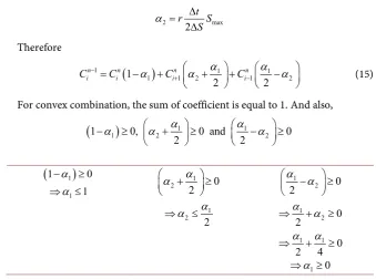
    (15)

For convex combination, the sum of coefficient is equal to 1. And also,

(

)

1 1

1 2 2

1 0, 0 and 0

≥0

1 1

α

⇒ ≤

1

2 ₂ 0

α

 ₊ _≥

 

 

1

2 ₂

α α

⇒ ≤

1

2 0

2

α

_α

 ₋ _≥

 

 

1

2 0

2

α _α

⇒ + ≥

1 1 ₀

2 4

α α

⇒ + ≥

1 0

α

⇒ ≥

where, Smax =maxSi.

5. Numerical Results

Consider for purposes of graphical presentation the value of a call option with strike price K = 100. The risk-free interest rate r = 0.12, the time to expiration is

T = 1 measured in years, and the volatility is = 0.10. The value of the call option is plotted over a range of stock prices 70≤ ≤S 130_{surrounding the strike price}

[image:6.595.201.541.68.320.2] [image:6.595.210.536.492.691.2]

is illustrated in Figure 1.

Figure 1 is produced by MATLAB. The figure shows the price of the stock at different time.

Figure 1. Numerical solution for European call at different time steps with K = 100, r = 0.12, σ = 0.1, T = 1.

70 80 90 100 110 120 130

0 5 10 15 20 25 30 35 40 45

Stock price

O

pt

ion pr

ic

e

(7)

[image:7.595.209.537.263.446.2] [image:7.595.209.537.492.691.2]

DOI: 10.4236/jmf.2018.82024 378 Journal of Mathematical Finance Figure 2 is the analytic solution of the Black-Scoles model for the same para-meters as before is.

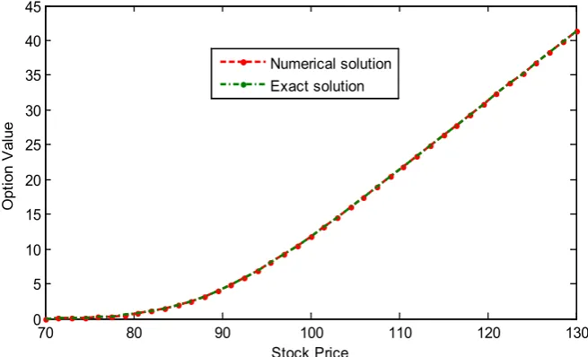
If the above two figures are combined into one, one can easily examine how the analytical and numerical solutions differ with each other. For identification, two different colors were used. Here the values of T, r, K, σ are same as previousand the temporal grid size ∆t = 0.01, and spatial grid size ∆S = 1.50.

From Figure 3, it is observed that the two solutions are almost superimposed. The red color represents the numerical solution and green represents the analytic solution. Two solutions cannot be distinguished by the naked eye. Hence the nu-merical scheme has a very small error.

Now to find the relative error for the scheme, the computation of the relative error in L1-norm which is defined by

Figure 2. Analytic solution for European call at different time steps with K = 100, r = 0.12, σ = 0.1, T = 1.

Figure 3. Analytic solution and Numerical solution at initial time (K = 100, r = 0.12, σ = 0.1, T = 1).

70 80 90 100 110 120 130

0 5 10 15 20 25 30 35 40 45

Stock price

O

pt

ion pr

ic

e

time remaining to expiration =1 yr time remaining to expiration =0.8 time remaining to expiration =0.6 time remaining to expiration =0.4 time remaining to expiration =0.2 time remaining to expiration =0

70 80 90 100 110 120 130

0 5 10 15 20 25 30 35 40 45

Stock Price

O

pt

ion V

al

ue

(8)

DOI: 10.4236/jmf.2018.82024 379 Journal of Mathematical Finance

1 1

e n

e C C err

C

− =

where Ce is the analytic solution and Cn is the numerical solution of Black-Scholes model for European call option. We perform our numerical scheme for t = 0 to 1, r = 0.12, K = 100, σ = 0.10 with temporal grid size ∆t = 0.0500 and spatial grid size ∆S = 3 which satisfy the stability conditions.

The relative error is shown in Figure 4.

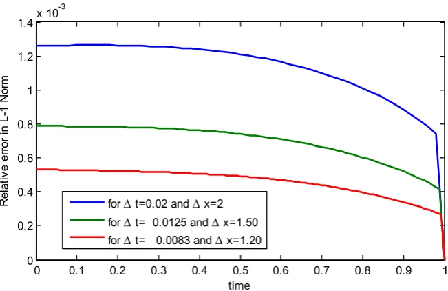
[image:8.595.210.538.271.448.2]

From Figure 4 it is seen that as time t goes from 0 to 1, the relative error be-comes smaller and smaller. For explicit difference scheme, the relative error is less than 0.0035 which is quite acceptable. Figure 5 represents that the error is de-creasing with respect to the smaller discretization parameters ∆t and ∆S, which shows the convergence of the explicit difference scheme.

Figure 4. Relative error for explicit difference scheme in the order of 10−3_.

Figure 5. Relative error of explicit difference scheme for different temporal and spatial grid size in the order of 10−3_.

0 0.1 0.2 0.3 0.4 0.5 0.6 0.7 0.8 0.9 1

0 0.5 1 1.5 2 2.5 3

3.5x 10

-3

time

Rel

at

ive er

ror

in

L-1 N

or

m

Relative error for ∆ t= 0.0500 and ∆ x=3

0 0.1 0.2 0.3 0.4 0.5 0.6 0.7 0.8 0.9 1

0 0.2 0.4 0.6 0.8 1 1.2

1.4x 10

-3

time

R

el

at

iv

e er

ror

in

L-1 N

or

m

for ∆ t=0.02 and ∆ x=2

for ∆ t= 0.0125 and ∆ x=1.50

[image:8.595.210.536.479.690.2]

(9)

[image:9.595.206.541.91.192.2]

Table 1. Comparison between the semi-implicit method and explicit method.

Stock Price Semi-implicit method Explicit method Exact value

4 1.631276e−06 1.168605e−06 1.067322e−06

8 0.146176 0.149235 0.149335

10 0.906372 0.916098 0.916291

16 6.236436 6.252282 6.252287

20 10.223892 10.246901 10.247014

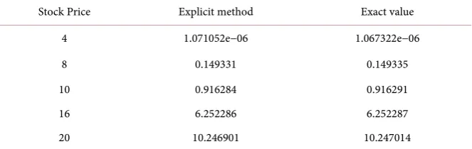
Table 2. Approximate value by explicit centered method and the exact value.

Stock Price Explicit method Exact value

4 1.071052e−06 1.067322e−06

8 0.149331 0.149335

10 0.916284 0.916291

16 6.252286 6.252287

20 10.246901 10.247014

6. Comparison with Other Numerical Scheme

In this section, a comparison is made between our explicit difference scheme with another numerical scheme that was used in finding the approximate solution of Black-Scholes model which is Semi-implicit method [5].

For a European call option with 0≤ ≤S 20_,_T_{= 0.25,}_K_{= 10,}_r_{= 0.1,}_σ_{= 0.4,}

with temporal grid size N = 2000 and spatial grid size M = 200, the Semi-implicit method and Explicit method were used to set the table below.

From Table 1 it is seen that explicit scheme gives better results than semi-implicit method. But the results obtained by the scheme that was developed here are not much close to the exact value. But if the temporal grid points are in-creased up to N = 41,000, spatial grid points up to M = 1000 and set the other pa-rameters value as above then the following values (Table 2) were found for dif-ferent stock prices.

7. Conclusion

[image:9.595.207.539.224.329.2]

(10)

References

[1] Black, F. and Scholes, M. (1973) The Pricing of Options and Corporate Liabilities. Journal of Political Economy, 81, 637-654. https://doi.org/10.1086/260062

[2] Merton, R.C. (1973) Theory of Rational Option Pricing. The Bell Journal of Eco-nomics and Management Science, 4, 141-183. https://doi.org/10.2307/3003143

[3] Jodar, L., Sevilla-Peris, P., Cortes, J.C. and Sala, R. (2005) A New Direct Method for Solving the Black-Scholes Equation. Applied Mathematics Letters, 18, 29-32.

https://doi.org/10.1016/j.aml.2002.12.016

[4] Company, R., Gonzalez, A.L. and Jodar, L. (2006) Numerical Solution of Modified Black-Scholes Equation Pricing Stock Options with Discrete Dividend. Mathemati-cal and Computer Modeling, 44, 1058-1068.

https://doi.org/10.1016/j.mcm.2006.03.009

[5] Dura, G. and Mosneagu, A.-M. (2010) Numerical Approximation of Black-Scholes Equation. An. Stiint. Univ.”Al. I. Cuza” Iasi. Mat, 56, 39-64.

[6] Shinde, A.S. and Takale, K.C. (2012) Study of Black-Scholes Model and its Applica-tions. Procedia Engineering, 38, 270-279.

https://doi.org/10.1016/j.proeng.2012.06.035

[7] Smith, G.D. (1985) Numerical Solution of Partial Differential Equations: Finite Dif-ference Methods. Clarendon Press, Oxford.