Munich Personal RePEc Archive
Energy Efficiency and Directed Technical
Change: Implications for Climate
Change Mitigation
Casey, Gregory
Brown University
24 January 2017
Online at
https://mpra.ub.uni-muenchen.de/80473/
Energy Efficiency and Directed Technical Change:
Implications for Climate Change Mitigation
Gregory Casey
July 2017
Abstract
In this paper, I construct a putty-clay model of directed technical change and use it to analyze the effect of environmental policy on energy use in the United States. The model matches key data patterns that cannot be explained by the standard Cobb-Douglas approach used in climate change economics. In particular, the model captures both the short- and long-run elasticity of substitution between energy and non-energy inputs, as well as trends in final-use energy efficiency. My primary analysis examines the impact of new energy taxes. The putty-clay model suggests that tax-inclusive energy prices need to be 273% higher than laissez-faire levels in 2055 in order to achieve policy goals consistent with international agreements. By contrast, the Cobb-Douglas approach suggests that prices need only be 136% higher. To meet the same goals, the putty-clay model implies that final good consumption must fall by 6.5% relative to a world without intervention, which is more than three times the prediction from the standard model. In a second analysis, I find that policy interventions cannot achieve long-run reductions in energy use without increasing prices, implying that energy efficiency mandates and R&D subsidies have limited potential as tools for climate change mitigation. Finally, I use the model to analyze the long-run sustainability of economic growth in a world with non-renewable resources. Using two definitions of sustainability, the new putty-clay model delivers results that are more optimistic than the existing literature.
KeywordsEnergy, Climate Change, Directed Technical Change, Growth
JEL Classification CodesO30, O44, H23
1
Introduction
To address global climate change, it is crucial to understand how carbon emissions will respond to policy interventions. Changes in energy efficiency will be an important component of this response. Indeed, rising energy efficiency – rather than the use of less carbon intensive energy sources – has been the major force behind the decline in the carbon intensity of output in the United States over the last 40 years (Nordhaus,2013). Thus, energy efficiency will almost certainly be a critical factor in any future approach to mitigating climate change.
Integrated assessment models (IAMs) are the standard tool in climate change economics. They combine models of the economy and climate to calculate optimal carbon taxes. The leading models in this literature frequently treat energy as an input in a Cobb-Douglas aggregate production func-tion (e.g.,Nordhaus and Boyer,2000;Golosov et al.,2014).1 Despite the significant insights gained from the IAMs, there are two restrictive assumptions in this approach to modeling energy. First, in response to changes in energy prices, the Cobb-Douglas approach allows immediate substitution between capital and energy, which is at odds with short-run features of the U.S. data (Pindyck and
Rotemberg, 1983;Hassler et al.,2012,2016b). This suggests that the standard approach may not
fully capture the effect of new taxes that raise the effective price of energy. Second, technological change is exogenous and undirected in the standard model. A substantial literature, however, sug-gests that improvements in energy-specific technology will play a pivotal role in combating climate change and that environmentally-friendly research investments respond to economic incentives (e.g.,
Popp et al.,2010;Acemoglu et al.,2012).
In this paper, I construct a putty-clay model of directed technical change that matches several key features of the data on U.S. energy use. In particular, the model captures both the short-and long-run elasticity of substitution between energy short-and non-energy inputs, as well as trends in final-use energy efficiency. In the model, each piece of capital requires a fixed amount of energy to operate at full potential. Technical change, however, can lower this input requirement in the next iteration of the capital good, or it can increase the ability of the next iteration to produce final output.2,3 When the price of energy increases relative to other inputs, firms invest more in energy
1Research on the human impact of climate change is large and spans many disciplines (Weyant,2017). I focus on the economics literature building on the neoclassical growth model, where both energy use and output are determined in general equilibrium. Many prominent IAMs take output to be exogenous or abstract from modeling energy use (e.g., Hope, 2011; Anthoff and Tol, 2014). Another strand of the climate change literature uses large computable general equilibrium (CGE) models. Of particular relevance to the current paper are analyses using the EPPA (Morris
et al.,2012) or Imaclim (Crassous et al.,2006) models, each of which has elements of putty-clay production.
2Capital good producers turn raw capital, ‘putty,’ into a capital good with certain technological characteristics,
including energy efficiency. While energy efficiency can be improved by research and development, there is no substitution between energy and non-energy inputs once the capital good is in operation, capturing the rigid ‘clay’ properties of installed capital.
3The literature on putty-clay production functions has a long history (e.g.,Johansen,1959;Solow,1962;Cass and
Stiglitz,1969;Calvo,1976). Of particular relevance is work byAtkeson and Kehoe(1999) who investigate the role of
putty-clay production in explaining the patterns of substitution between energy and non-energy inputs in production. The older literature on putty-clay models focuses on choosing a type of capital from an existing distribution or on the simultaneous use of old and new vintages. The current paper focuses on how the cutting-edge of technology, which is embodied in capital goods, evolves over time. As discussed in the next section, this modeling approach draws insight
efficiency and less in other forms of technology. In the long-run, the endogenous research activity leads to a constant expenditure share of energy, even though there is no short-run substitution between energy and non-energy inputs.
The model also matches the source of gains in energy efficiency. In particular, I show that the declines in the carbon and energy intensities of output in the U.S. have been driven by reductions in final-use energy intensity. In other words, energy efficiency improves when capital goods and consumer durables require less energy to run, not when the energy sector becomes more efficient at turning primary energy (e.g., coal) into final-use energy (e.g., electricity). Moreover, these energy efficiency improvements have been more important than substitution between energy sources in explaining the historical trend towards cleaner production. The putty-clay model examines this crucial margin of technological progress, which has not received much attention in the existing literature on the environment and directed technical change (e.g.,Acemoglu et al.,2012,2016). To capture changes in final-use energy efficiency, I construct a new directed technical change model in which innovation occurs in different characteristics of capital goods. This new model yields different research incentives than the seminal approach ofAcemoglu (1998,2002), where innovation occurs in different sectors.
The new putty-clay model allows for a simple and transparent calibration procedure. It re-sembles the neoclassical growth model in several important ways, implying that many parameters are standard and can be taken from the existing literature. I calibrate the innovation and energy sectors to aggregate U.S. data on economic growth and fossil fuel energy use. I then use the model to perform three exercises. In my primary exercise, I examine the effect of energy taxes on energy use and compare the results to the standard Cobb-Douglas approach. I also analyze whether it is possible for policies, such as R&D subsidies or efficiency mandates, to reduce long-run energy use without raising the price of energy. Finally, I asses how the presence of non-renewable resources effects the potential for economic growth to be sustained in the very long run.
Both the Cobb-Douglas and putty-clay models are consistent with long-run features of the U.S. data. As a result, they have identical predictions for long-run energy use in the absence of climate policy. Their predictions for the impact of climate policy, however, differ significantly. In the long run, both models predict that energy expenditure share of output will be constant. When new taxes raise the effective price of energy, however, the Cobb-Douglas model assumes that capital and labor can be quickly substituted for energy, leaving the expenditure share unchanged. In contrast, the putty-clay model predicts that the expenditure share will slowly evolve as the result of purposeful research activity. As a result, the energy expenditure share will be higher on the transition path and may converge to a permanently higher long-run level. Compared to the standard approach, therefore, the putty-clay model predicts that higher energy taxes are needed to achieve a desired reduction in energy use. This analysis shows that constraining the model match short-run features of the data can greatly alter the predicted long-run reactions to environmental policy.
These differences are quantitatively important. The new model suggests that tax-inclusive energy prices need to be 273% higher than laissez-faire levels in 2055 in order to achieve policy goals consistent with the Paris Agreement.4 By contrast, the standard Cobb-Douglas approach
suggests that tax-inclusive energy prices need only be 136% higher. To meet the same goals, the putty-clay model implies that final good consumption must fall by 6.5% relative to a world without intervention, which is more than three times the prediction from the standard model. Thus, compared to the standard approach, the new model predicts that greater taxation and more forgone consumption are necessary to achieve environmental policy goals. When applying the same taxes to both models, the new putty-clay model of directed technical change predicts 24% greater cumulative energy use over the next century. This indicates that policy designed with the Cobb-Douglas model will yield significantly different environmental results in a world better represented by the new putty-clay model.
Research subsidies and efficiency mandates are commonly used in attempts mitigate climate change and achieve energy security (Gillingham et al.,2009;Allcott and Greenstone,2012). Despite their popularity, these policies may be ineffective due to rebound effects. Rebound occurs when economic behavior lessens the reduction in energy use following efficiency improvements. A long existing literature attempts to indirectly evaluate the effectiveness of such policies by estimating the size of rebound effects, usually in partial equilibrium or static settings.5 The new putty-clay model,
however, makes it possible to directly analyze the broader motivating question: can policies that improve energy efficiency achieve long-term reductions in energy use, even if they do not increase energy prices? I start by considering the standard rebound exercise of a one-off improvement in energy efficiency. Such shocks lead to short-run reductions in energy use, but also lower the incentive for future investment in energy efficient technology. As a result, the interventions lead to temporary increases in medium-term energy use relative to world without policy, an extreme form of rebound known as ‘backfire.’ Eventually, the short-term reductions and medium-term backfire offset each other, leaving cumulative energy use unchanged. Permanent policy interventions can overcome rebound effects to achieve long-run reductions in energy use relative to laissez-faire, but cannot achieve absolute decreases in energy use. Thus, the model suggests that policies that do not raise the price of energy will be unable to meet long-run environmental policy goals.
I also examine the sustainability of economic growth in a world with non-renewable resources. Using two different versions of sustainability, I find results that are more optimistic than the existing literature. The first – and more standard – definition ignores climate change and is concerned with the ability of an economy to maintain current levels of consumption growth. Focusing on models
4In particular, I simulate taxes needed to reduce energy use to 60% of 2005 levels by the year 2055. This is
consistent with goals laid out in the Paris Agreement, which suggests that the United States adopt policies consistent with a 80% reduction in carbon emissions by 2050. Thus, I examine a case where half of the required reduction in carbon emissions comes from reductions in energy use. The goals are outlined in the Intended Nationally Determined Contribution (INDC) submitted by the United States to the United Nations Framework Convention on Climate Change (UNFCC), which is available at: http://www4.unfccc.int/submissions/INDC/Published%20Documents/ United%20States%20of%20America/1/U.S.%20Cover%20Note%20INDC%20and%20Accompanying%20Information.pdf.
with exhaustible resources, the existing DTC literature suggests that this form of sustainability is impossible because energy use is currently increasing, which is not possible in the long run (e.g.,
Andr´e and Smulders, 2014; Hassler et al., 2012, 2016b). I consider the case where resources are
inexhaustible, but only accessible at increasing and unbounded extraction costs,6 a formulation that captures the abundance of coal and the potential to exploit ‘unconventional’ sources of oil and natural gas (Rogner, 1997; Rogner et al., 2012). In this setting, I find that energy use will necessarily increase in the long run (in the absence of policy intervention), implying that the presence of non-renewable resources alone does not pose a threat to this form of sustainability. The second definition of sustainability asks whether environmental policy can keep the stock of pollution low enough to prevent an ‘environmental disaster.’ The existing literature suggests that this form of sustainability is impossible when polluting and non-polluting factors of production are complements (Acemoglu et al., 2012). By considering the ability of new technologies to save on dirty inputs, I show that it is possible for policy to prevent an environmental disaster, even in the case of perfect complementarity.
The rest of this paper is structured as follows. Section 2surveys the related literature. Section
3 discusses the empirical motivation underlying the theory. The model is presented in Section 4
and the calibration in Section 5. Section 6 reports the results of the quantitative analyses, and Section7 concludes.
2
Related Literature
As described above, this paper contributes to the literature on climate change economics that takes a Cobb-Douglas approach to energy modeling in IAMs. This paper is also closely related to a growing literature demonstrating that directed technical change (DTC) has important implications for environmental policy. These studies generally focus on clean versus dirty sources of energy, rather than energy efficiency. Acemoglu et al. (2012) demonstrate the role that DTC can play in preventing environmental disasters and emphasize the elasticity of substitution between clean and dirty production methods. The model in this paper bears more resemblance to an ‘alternate’ approach they mention where firms can invest in quality improvements or carbon abatement, where the latter only occurs in the presence of carbon taxes. Several other studies also investigate the case where policy interventions affect how technological change is directed between production and abatement activities.7 Lemoine (2017) demonstrates how the transition between sources of energy
is affected by both innovation and increasing extraction costs in a world where new innovations are complementary to energy sources, but different energy sources are close substitutes. Aghion
et al. (2016) provide a static DTC model of clean and dirty innovation in the automotive industry
that includes an intra-product decision about energy efficiency. I build on these earlier works by
6Models with increasing extraction costs have a long history in economics (e.g.,Heal,1976;Solow and Wan,1976;
Pindyck,1978).
7See, for example,Hart(2008),Peretto (2008),Grimaud and Rouge(2008), andGans(2012). Hart(2004) and
Ricci(2007) consider the decision to investment in abatement technology in a model where technology is embodied
constructing a new model of directed technical change, focusing on energy efficiency, quantitatively investigating the macroeconomic effects of prominent environmental policies, and comparing the results to the standard approach taken in IAMs.8 I also provide evidence that ‘environmental
disasters’ can be averted even when polluting and non-polluting inputs are perfect complements, a result that is more optimistic than those in the existing DTC literature (Acemoglu et al.,2012).
Two recent papers extend the standard DTC model to quantitative investigation of macroeco-nomic policy (Acemoglu et al.,2016;Fried,forthcoming). Both focus on the issue of clean versus dirty energy sources and account for energy efficiency by calibrating growth in clean energy to overall de-carbonization of the economy. The current paper builds on these works by explicitly investigating energy efficiency as a separate source of innovation, using a new underlying model of DTC, and comparing the results to the standard approach taken in climate change economics.9
This paper is also related to the literature on DTC and energy use, which focuses on the efficiency of the energy transformation sector, rather than the energy requirements of capital goods. The literature begins with Smulders and De Nooij (2003) who apply the original DTC model directly to energy efficiency and use it to analyze the effects of exogenous changes in energy availability. Subsequent literature has focused on the relationship between DTC and the sustainability of long-run economic growth in the presence of exhaustible resources (e.g., Di Maria and Valente, 2008;
Andr´e and Smulders, 2014; Hassler et al., 2012, 2016b). I build on the existing literature by
constructing a new DTC model that focuses on final-use energy efficiency and by quantitatively examining the impacts of climate change mitigation policies. I also show how the prospects for long-run sustainability improve when considering the more empirically relevant case of inexhaustible resources and increasing extraction costs.10
The new putty-clay model of directed technical change builds on the aggregate social planner’s model of innovation and exhaustible resources developed byHassler et al.(2012, 2016b). In order to investigate the role of energy efficiency in climate change mitigation policy, the current model differs from their work in two key aspects. First, I construct a decentralized model with incentives for innovation, which is necessary to quantify the effects of policy and to account for externalities. Rather than importing the seminal directed technical change model developed byAcemoglu(1998,
8A related and influential literature looks at induced, but not directed, technical change and its implications for
climate policy. These models tend to focus on social planner problems. Key contributions in this literature include
Goulder and Schneider(1999),Goulder and Mathai(2000),Sue Wing(2003), andPopp(2004).
9It is also important to note that the DTC literature is supported by microeconomic studies that investigate
the presence of directed technical change. Newell et al.(1999) andJaffe et al.(2003) demonstrate that the energy efficiency of energy intensive consumer durables (air conditioners and gas water heaters) responds to changes in prices and government regulations, providing evidence for the existence of directed technical change. Similarly,Popp (2002) finds that energy efficiency innovation, as measured by patents, responds to changes in energy prices. He looks at both innovations in the energy sector and in the energy efficiency characteristics of other capital goods. More recently, Dechezleprˆetre et al.(2011) and Calel and Dechezlepretre (2016) find that patents for ‘low carbon’ technologies, which include more energy efficient and less carbon intensive innovations, respond to both energy prices and public policies designed specifically to address climate change. Aghion et al.(2016) find that government policies have a strong effect on energy efficient research in the automotive sector.
10Peretto and Valente(2015) focus on another form of sustainability, the growth of population in a world with a
2002), I take a new approach in which innovation occurs in different characteristics of capital goods, not in different sectors. As discussed in Section 3, the new approach is motivated by data on U.S. energy use. Second, I consider the case of infinite potential supplies of energy and increasing extraction costs. The potentially infinite supply of energy incorporates the role of coal in fossil fuel energy use11and the possibility for new methods of resource extraction to become feasible as costs rise (Rogner,1997; Rogner et al.,2012). Moreover, the model of DTC and increasing extraction costs predicts that, in the absence of policy, energy use will increase in the long run. This is consistent with data and a first-order concern for climate policy, but contrary to the predictions of models with only exhaustible resources. More generally, the goal of climate change policy is to avoid using all available fossil fuels, implying that the optimal management of exhaustible resources in not a primary concern in this context (Covert et al.,2016).
This study is also related to the literature on the rebound effect, which can be thought of in two parts: a microeconomic literature that estimates rebound effects for specific goods12 and a macroeconomic literature that investigates static general equilibrium effects.13 By studying this question in the context of a growth model, I incorporate several factors that are generally excluded from the literature. Most importantly, the putty-clay model incorporates the effects of changes in energy efficiency on subsequent innovation, a neglected issue thatGillingham et al.(2015) describe as a ‘wild card’ in our understanding of the long-run effects of energy efficiency policies. Moreover, the existing macroeconomic rebound literature focuses heavily on the elasticity of substitution between energy and non-energy inputs in production (e.g., Sorrell et al., 2007; Borenstein et al.,
2015; Lemoine, 2016). The putty-clay model of directed technical change allows the elasticity to
vary over time, matching key features of U.S. data on energy use. The model also accounts for the cost of achieving energy efficiency,14 as well as long-run changes in energy extraction costs and capital accumulation, none of which has received much attention in the existing quantitative literature.
3
Empirical Motivation
In this section, I discuss patterns in the data that motivate the theoretical choices made in this paper. In particular, I present evidence that a) declines in the final-use energy intensity of output drive reductions in the carbon intensity of output, b) there is a very low short-run elasticity of substitution between energy and non-energy inputs, and c) there is no long-run trend in the energy expenditure share of final output.
11Coal is predicted to to be the primary driver of global carbon emissions and is available in abundant supply
(van der Ploeg and Withagen,2012;Golosov et al.,2014;Hassler et al.,2016a).
12See, for example,Allcott(2011) andJessoe and Rapson(2014), amongst others.
13See Lemoine(2016) for a recent theoretical treatment of rebound. For quantitative results from CGE models,
seeTurner(2009) andBarker et al.(2009), amongst others.
To analyze the determinants of the carbon intensity of output, I consider the following decom-position:
CO2
Y =
CO2 Ep
·Ep
Ef ·Ef
Y , (1)
where CO2 is yearly carbon emissions, Y is gross domestic product, Ep is primary energy use
(e.g., coal, oil), and Ef is final-use energy consumption (e.g., electricity, gasoline). The carbon
intensity of primary energy, CO2E
p , captures substitution between clean and dirty sources of energy
(e.g., coal versus solar). The efficiency of the energy sector, which transforms primary energy into final-use energy, is captured by Ep
Ef. For example, the ratio decreases when power plants become
more efficient at transforming coal into electricity. The final-use energy intensity of output, Ef
Y ,
measures the quantity of final-use energy used in production and consumption. For example, the ratio decreases when manufacturing firms use less electricity to produce the same quantity of goods. The results of this decomposition are presented in Figure 1, which plots the carbon intensity of output and each component from equation (1) for the United States from 1971-2014. Data are normalized to 1971 values.15 The carbon intensity of output fell over 60% during this time period, and this decline is matched almost exactly by the decline in the final-use energy intensity of output. The carbon intensity of primary energy, CO2E
p , declined approximately 15% over this period. While
this is a significant improvement for environmental outcomes, it is relatively small compared to the overall improvements in the carbon intensity of output. Finally, the efficiency of the energy transformation sector, as measured by the inverse of Ep
Ef, actually declined roughly 15% over this
period.16
Motivated by this evidence, I construct a model that focuses on the final-use energy intensity of output. This creates a significant break with existing work. Existing macroeconomic research on directed technical change and climate change focuses on clean versus dirty sources of energy and does not consider energy efficiency as a distinct source of innovation (e.g., Acemoglu et al., 2012,
2016;Fried,forthcoming). Transition to cleaner energy sources will undoubtedly be an important
component of any approach to mitigate climate change, but the historical data strongly suggest that improved energy efficiency will be a pivotal aspect of any policy response. At the same time, applying the seminal DTC model of Acemoglu (1998, 2002) to the question of energy efficiency would require focusing on the efficiency of the energy sector (e.g., Smulders and De Nooij, 2003;
Andr´e and Smulders,2014).17 Thus, I construct a new model where energy efficiency is driven by the
energy requirements of capital goods. This theoretical innovation significantly alters the underlying
15Appendix SectionAdescribes the data and provides links to the original sources.
16This result is driven by differences in the efficiency of transformation across different sources of primary energy,
rather than technological regress.
17Existing work on induced technical change in social planner models also focuses on the efficiency of the energy
0 20 40 60 80 100 120
[image:10.612.168.438.72.261.2]1970 1975 1980 1985 1990 1995 2000 2005 2010 CO2/Y CO2/Ep Ep/Ef Ef/Y
Figure 1: This figure decomposes the decline in the carbon intensity of output. CO2 is yearly carbon emissions,
Y is GDP, Ep is primary energy, andEf is final-use energy. This figure demonstrates that the fall in the carbon
intensity of output, CO2
Y , has been driven by decreases in final-use energy intensity of output, Ef
Y , rather than the use
of cleaner energy sources, CO2
Ep , or a more efficient energy transformation sector,
Ep
Ef. Data are from the International
Energy Agency (IEA) and the Bureau of Economic Analysis (BEA). All values are normalized to 1971 levels.
incentives for research and development, implying that it is important to consider energy efficiency as a distinct source of innovation.18
Figure 2 provides evidence on the elasticity of substitution between energy and non-energy inputs. In particular, it shows the expenditure share of energy (Eshare), the primary energy intensity
of output (Ep
Y ), and the average real energy price use in the United States from 1971-2014.19 The
data indicate that expenditure, but not energy intensity, reacts to short-term price fluctuations, suggesting that there is very little short-run substitution between energy and non-energy inputs. At the same time, there is no trend in the energy expenditure share of output, despite increasing prices. This pattern suggests that there is a constant long-run expenditure share in the absence of fundamental changes in parameters or policy, and equivalently, that the long-run elasticity of substitution between energy and non-energy inputs is close to one. The model in this paper will match both the short- and long-run patterns facts. Hassler et al. (2012,2016b) provide a formal maximum likelihood estimate of the short-run elasticity of substitution between energy and non-energy inputs. They find an elasticity of substitution very close to zero. For the purposes of this paper, I will treat the elasticity as exactly zero and use a Leontief production structure, which allows
18Of course, not all improvements in energy efficiency need to driven by technical change. In particular, sectoral
reallocation could explain aggregate changes in energy use. Decomposition exercises suggest that improvements in intra-sectoral efficiency, rather than reallocation, have been the key driver of falling energy intensity over this period
(Sue Wing,2008;Metcalf,2008). They also suggest that, prior to 1970, sectoral reallocation was the primary driver
of falling energy intensity. The calibration will focus on the post-1970 period. Existing work suggests that there was a significant regime shift in both energy prices and energy efficiency improvements after this period (e.g.,Hassler
et al.,2012,2016b;Baumeister and Kilian,2016;Fried,forthcoming).
0 50 100 150 200 250
[image:11.612.169.437.78.260.2]1970 1975 1980 1985 1990 1995 2000 2005 2010 Ep/Y Real Energy Price Eshare
Figure 2: This figure demonstrates that short-run movements in energy prices affect the energy expenditure share of output (Eshare) in the short-run, but not the energy intensity of output (EYP). At the same time, there is no
long-run trend in the energy expenditure share of output, despite increasing prices. Data are taken from the Energy Information Administration (EIA) and the Bureau of Economic Analysis (BEA). All values are normalized to 1971 levels.
for the construction of a tractable putty-clay model with innovation in capital good characteristics. They also find that energy efficiency increases after prices rise, suggesting a DTC model of the type investigated here.20
The trendless expenditure share of energy in Figure 2 serves as the motivation for the Cobb-Douglas production function in IAMs (Golosov et al., 2014; Barrage, 2014). At the same time, the analysis by Hassler et al. (2012, 2016b) suggests that the long-run energy expenditure share – which will eventually be constant – must be significantly higher than the current level. The model developed in this paper bridges the gap between these two approaches. It yields a constant energy expenditure share that matches the current level, while simultaneously replicating both short- and long-run patterns of substitution. Moreover, the analysis shows how constructing a model that matches both short- and long-run features of data significantly alters the predicted long-run reactions to climate policy. In particular, the putty-clay model suggests that higher taxes
20As demonstrated in Figure 2, the price of energy in the United States had an upward trend from 1971-2014.
Once again, this is a good match for post-1970 data, but not for U.S. data in the preceding two decades, where energy prices actually declined. Consistent with the predictions of the model, decomposition exercises suggest that intra-sectoral energy efficiency declined during this period of falling prices (Sue Wing,2008). In this paper, I focus on the case where prices increase in the long run, though this is not central to any of the policy analysis. Increasing prices are consistent with theoretical work based on the Hotelling problem or increasing extraction costs (e.g.,Hotelling,
1931;Heal,1976;Pindyck,1978), as well as empirical work suggesting a U-shaped pattern in long-run energy prices
and more forgone consumption are necessary to meet environmental policy goals when compared to the Cobb-Douglas model, which is only consistent with long-run patterns in the data.
4
Model
4.1 Structure
4.1.1 Final Good Production
Final good production is perfectly competitive. The model extends the standard endogenous growth production function to account for energy use. To match the extremely low short-run elasticity of substitution between energy and non-energy inputs, I will consider a Leontief structure
Qt = Z 1
0
min[ AN,t(i)Xt(i) α
L1−α
t , AE,t(i)Et(i)]di, (2)
s.t. AE,t(i)Et(i)≤AN,t(i)Xt(i)αL1t−α ∀i, (3)
whereQtis gross output at timet,AN,t(i) is the the quality of capital goodi,Xt(i) is the quantity
of capital good i, Lt is the aggregate (and inelastic) labor supply, AE,t(i) is the energy efficiency
of capital good i, and Et(i) is the amount of energy devoted to operating capital good i. Several
components of the production function warrant further discussion. As in the standard endogenous growth production function, output is generated by a Cobb-Douglas combination of aggregate labor, Lt, and a series of production process, each of which uses a different capital good, indexed
byi. Unlike the endogenous growth literature, each production process also requires energy to run. Thus, the usual capital-labor composite measures the potential output that can be created using each production process, and the actual level of output depends on the amount of energy devoted to each process, Et(i). The notion of potential output is captured by constraint (3). Each capital
good i has two distinct technological characteristics. The quality of the capital good, AN,t(i),
improves its ability to produce output, and the energy efficiency of the capital good,AE,t(i), lowers
the amount of energy needed to operate the production process at full potential.21,22
4.1.2 Energy Sector
Energy is available in infinite supply, but is subject to increasing extraction costs (see, e.g., Heal,
1976;Pindyck,1978;Lin and Wagner,2007). Extraction costs are paid in final goods, and energy
is provided by a perfectly competitive sector with open access. The increasing extraction cost
21Consistent with the econometric literature on energy use, energy requirements depend both on the amount of
capital and the amount of labor being used in the production process (Van der Werf, 2008; Hassler et al., 2012,
2016b). Second, consistent with both the econometric and DTC literatures, improvements in non-energy technology,
AN(i), raise energy requirements (e.g.,Smulders and De Nooij,2003;Van der Werf,2008;Hassler et al.,2012,2016b;
Fried,forthcoming).
22Appendix SectionB.6.2presents as equivalent formulation for final good production that highlights the continuity
incorporates two main forces that govern long-run energy availability. First, it captures the increase in cost needed to extract conventional energy resources from harder-to-access areas.23 Second, it captures the increase in cost that may occur when a particular energy source is exhausted, necessitating a switch to a type of energy which is more difficult to extract. In particular, the infinite supply of energy and increasing extraction costs capture the existence of ‘unconventional’ energy sources, which have high extraction costs, but are available in vast quantities (Rogner,1997;
Rogner et al., 2012).24 As in Golosov et al. (2014), the treatment of energy sources as infinite in
potential supply also incorporates the abundance of coal, which is predicted to be the major driver of climate change (van der Ploeg and Withagen,2012;Hassler et al.,2016a).25
The marginal cost of extraction, which will also be equal to the price, is given by
pE,t = ξE¯tι−1, (4)
where ¯Et−1 is total energy ever extracted at the start of the period. The law of motion for the
stock of extracted energy is given by
¯
Et=Et−1+ ¯Et−1. (5)
Intuitively, energy producers exploit new sources of energy in each period and the difficulty of extraction is constant within each source.26,27
23For example, recent research suggests that most new oil production comes from the exploitation of new geographic
areas, rather than improved technology applied to existing sources of energy (Hamilton,2012).
24For example,Rogner et al.(2012) estimate a resource base of 4,900 – 13,700 exajoules (EJ) for conventional oil,
compared with annual production of 416 EJ across all energy sources. Thus, constraints on availability of conventional oil sources may be binding. The ability to exhaust fossil fuel energy sources, however, appears much less likely when considering other options. The resource base for unconventional sources of oil is estimated to be an additional 3,750 – 20,400 EJ. Meanwhile, the resource base for coal and natural gas (conventional and unconventional) are 17,300– 435,000 EJ and 25,100 – 130,800 EJ, respectively. These estimates rely on projections regarding which resources will be profitable to extract from the environment. When considering the full range of energy sources that could become profitable to extract as resource prices tend towards infinity, the numbers grow even larger. In particular, such ‘additional occurrences’ are estimated to be larger than 1 million EJ for natural gas and 2.6 million EJ for uranium.
25Technically,Golosov et al.(2014) specify a finite amount of coal, but assume it is not fully depleted. Thus, it has no scarcity rent, although it does have an extraction cost. Oil, by contrast, is assumed to have no extraction cost, but does have a positive scarcity rent. Hart and Spiro (2011) survey the empirical literature and find little evidence that scarcity rents are a significant component of energy costs. They suggest that policy exercises focusing on scarcity rents will give misleading results.
26This is consistent, for example, with recent evidence from the oil industry, where drilling, but not within-well
production, responds to changes in prices (Anderson et al.,2014).
4.1.3 Final Output
Final output is given by gross production less total energy extraction costs, which are equal to energy expenditures by the final good producer. As long as equation (3) holds with equality,28final output is given by
Yt = L1t−α Z 1
0
1− pE,t
AE,t(i)
AN,t(i)Xt(i)α di. (6)
This formulation further illuminates the continuity between the production function used here and the standard approach in endogenous growth models. Output has the classic Cobb-Douglas form with aggregate labor interacting with a continuum of capital goods. As in the endogenous growth literature, this structure maintains tractability in the putty-clay model, despite the Leontief nature of production.
Final output can either be consumed or saved for next period. In the empirical application, each period will be ten years. Following existing literature, I assume complete depreciation during production (Golosov et al.,2014). Thus, market clearing in final goods implies
Yt=Ct+Kt+1 =Ltwt+rtKt+ Πt+pRt +Tt, (7)
where Kt is aggregate capital, Πt is total profits, Tt is the net government budget, and pRt is
total payments to R&D inputs (discussed in the next section). When examining the effects of environmental policy, I assume that the government balances the budget using lump-sum taxes or transfers.
4.1.4 Capital Goods and Research
Each type of capital good is produced by a single profit-maximizing monopolist in each period. This monopolist also undertakes in-house R&D activities to improve the embodied technological characteristics, AN,t(i) and AE,t(i). The R&D production function is given by
AJ,t(i) =
1 +ηJRJ,t(i)R−J,tλ
AJ,t−1, J ∈ {N, E}, (8)
whereRJ,t(i) is R&D inputs assigned to characteristic J by firm iin periodt,RJ,t≡R01RJ,t(i)di,
and AJ,t−1 ≡max{AJ,t−1(i)}. In words, R&D builds on aggregate knowledge,AJ,t−1, and current
period within-firm research allocations,RJ,t(i), but is also subject to a congestion externalityR
−λ
J,t
caused by duplicated research effort. When the period ends, patents expire and the best technology becomes available to all firms. Monopolists make decisions to maximize single period profits.29
28To ensure that equation (3) holds with equality, it is sufficient, but not necessary, to assume that capital fully
depreciates after each period. If capital fully depreciates, then in equilibrium forward looking consumers will never ‘over-invest’ in capital and drive its return to zero. This assumption will be maintained in the empirical analysis, which uses a time period of ten years, and is also employed inGolosov et al.(2014).
29This can be motivated in several ways. Most directly, the identity of the firm producing capital good icould
There are a unit mass of R&D inputs, yielding30
RN,t+RE,t = 1 ∀t. (9)
I assume that the investment price is fixed at unity. Thus, market clearing implies that
Z 1
0
Xt(i)di=Kt, (10)
whereKt is aggregate capital.
4.1.5 Consumer Problem
The consumer side of the problem is standard. In particular, the representative household chooses a path of consumption such that
{Ct}∞t=0 = argmax ∞
X
t=0 βtLt
˜
c1−σ
t
1−σ, (11)
where ˜ct=Ct/Lt. Population growth is given exogenously by
Lt+1= (1 +n)Lt. (12)
I am interested in the decentralized equilibrium. Thus, I consider the case where the representative household takes prices and technology as given. In other words, the household’s budget constraint is given by the second equality in (7).
4.2 Analysis
As demonstrated in Appendix Section B.1, the first order conditions for the final good producer yield the following inverse demand functions:
pX,t(i) = αAN,t(i)α
1− τtpE,t
AE,t(i)
L1−α
t Xt(i)α−1, (13)
wt = (1−α)1−
τtpE,t
AE,t(i)
L−α
t AN,t(i)Xt(i)α, (14)
reasonable considering the ten year period length. The set-up presented here is isomorphic to one where firms are infinitely lived and the aggregate technology, AJ,t−1, is given by the average of the previous period‘s technology as
inFried (forthcoming). This would open up the possibility of technological regress, though it would not occur in
equilibrium.
30This is consistent with both existing literature on DTC and the environment (Acemoglu et al., 2012; Fried,
forthcoming) and the social planner model provided by (Hassler et al., 2012, 2016b). Often, models of directed
where τt≥1 is a proportional tax on energy. The intuition for the result is straightforward. The
final good producer demands capital goods until marginal revenue is equal to marginal cost. Unlike the usual endogenous growth model, marginal revenue is equal to marginal product minus the cost of energy needed to operate capital goods. Consider the case where the final good producer is already operating at a point where AN,t(i)Xt(i)
α
L1−α
t =AE,t(i)Et(i). If the final good producer
purchases more capital, it receives no increase in output unless there is a corresponding increase in energy purchased. The final good producer realizes this when making optimal decisions and adjusts demand for capital accordingly. This iso-elastic form for inverse demand maintains the tractability of the model.
Monopolist providers of capital goods must decide on optimal production levels and optimal research allocations. See Appendix SectionB.2for a formal derivation of the monopolists’ behavior. Given the iso-elastic inverse demand function, monopolists set price equal to a constant markup over unit costs. Since capital goods must be rented from consumers, the unit cost is given by the rental rate,rt. Thus, monopolist optimization yields
pX,t(i) =
1
αrt, (15)
Xt(i) = α 2 1−αr
−1
1−α
t AN,t(i)
α
1−αLt1−
τtpE,t
AE,t(i) 11
−α, (16)
¯
πX,t(i) = (
1
α −1)α
2 1−αr
−α
1−α
t AN,t(i)
α
1−αLt1− τtpE,t
AE,t(i) 11
−α, (17)
where ¯πX,t(i) is production profits (i.e., profits excluding research costs) of the monopolist.
To understand research dynamics, it is helpful to look at the relative prices for research inputs,
(1−ηS
t)pRE,t(i)
pR N,t(i)
= τtpE,tAN,t(i)
αAE,t(i)21−AτtE,tpE,t(i)
ηER−E,tλAE,t−1
ηNR−N,tλAN,t−1
, (18)
wherepR
J,t(i) is the rent paid to research inputs used by firmito improve technological characteristic
J at timetandηtS ∈[0,1) is a subsidy for energy efficient research. There are several forces affecting the returns to R&D investment. First, increases in the tax-inclusive price of energy increase the relative return to investing in energy efficiency. Second, the return to investing in a particular type of R&D is increasing in its efficiency. Research efficiency, in turn, depends on inherent productivity,
ηJ, accumulated knowledge, AJ,t−1, and the amount of congestion, R −λ
J,t. Third, since energy and
non-energy inputs are complements in production, increases inAN,t(i) raise the return to investing
inAE,t(i) and vice versa. These effects, however, are asymmetric. To maximize profits, monopolists
balance two forces that drive demand for their products: ‘output-increasing’ technological progress,
AN,t(i), and ‘cost-saving’ technological progress, AE,t(i). The asymmetry occurs because energy
efficiency, AE,t(i), has a negative and convex effect on the cost of energy per unit of final output, τtpE,t
Finally, the return to investing in the quality of capital goods is increasing in the share of final output paid to capital good producers,α.
In the usual DTC model, this analysis would demonstrate the role of market size and price effects in research incentives. As demonstrated in equation (18), however, aggregate inputs do not affect R&D decisions in this model. In other words, market size effects play no role in this model. This is due to the short-run complementarity between energy and non-energy inputs. Moreover, the price effects in this model differ from those in the usual DTC model. Since the price of the final good is the numeraire, τtpE,t
AE,t(i) is the cost of energy per unit of final good production, and 1−
τtpE,t
AE,t(i)
is the cost of non-energy inputs in final good production. Thus, the relative input prices do affect research allocations, but the relative price is completely determined by the cost of energy extraction. Moreover, as explained above, the relative price of energy – along with lagged technology levels – enter asymmetrically, unlike in the seminal model. These theoretical differences highlight the importance of considering the case where improvements in energy efficiency are driven by final-use energy, rather than using the more common approach where innovation occurs in different sectors. Given that all firms use common technology at the start of the period, they make identical R&D decisions and, as a result, they end the period with identical technology. Moreover, there is a unit mass of monopolists. Thus,RJ,t(i) =RJ,t ∀i, J, t. The optimal research allocations are given
by the implicit solution to (19) and (20),
RE,t =
q τ
tpE,t
AE,t−1
r 1
α(1−ηS t)
ηER−E,tλ
ηN(1−RE,t)−λ +ηER
−λ
E,t−ηER1
−λ
E,t
+ (1 +ηER1
−λ
E )−1
ηER−E,tλ
, (19)
RN,t = 1−RE,t. (20)
This formulation highlights the simple closed form solution in the special case where λ = 0 and
ηS
t = 0. To analyze the determinants of research activity, it is instructive to consider multiplying
both sides of (19) by ηER−E,tλ so that the growth rate of energy efficiency technology is given as
a function of the other parameters. Since ηSt ∈ [0,1), the left-hand side is strictly increasing in RE,t in this formulation and the right-hand side is strictly decreasing in RE,t. Thus, we can
note a few important partial effects. First, the level of non-energy technology does not affect the research allocation. The perfect complementarity in final good productions drives this result. As expected, increases in the tax-inclusive price of energy lead to increases in the fraction of research inputs devoted to advancing energy efficient technology. More surprisingly, increases in past energy efficiency lead to decreases in the amount of research effort devoted to energy efficiency, even though the research productivity builds on past knowledge. As in the case of non-energy research, this improvement in research productivity is exactly balanced by the complementary nature of production. In the case of energy efficiency, however, the convex relationship between energy efficiency and the effective cost of energy, τtpE,t
AE,t(i), creates further disincentive to invest in energy
Utility maximization yields
˜
ct
˜
ct+1 −σ
=βrt+1. (21)
Noting that all monopolists make the same decisions and that there is a unit mass of monopolists, the real interest rate is given by
rt = α2AαN,t
1−τtpE,t
AE,t
L1−α
t Kα
−1
t , (22)
where the market clearing condition from equation (10) has been applied.
4.3 Equilibrium
Definition 1. A competitive equilibrium is a sequence of prices, {wt, pX,t, rt, pRt , pE,t}∞t=0,
alloca-tions,{Ct, Kt, Lt, Et, RN,t, RE,t}∞t=0, technology levels,{AN,t, AE,t}∞t=0, and environmental policies,
{τt, ηtS}
∞
t=0, such that each of the following conditions holds ∀t:
• The economy obeys market clearing conditions for final goods, (7), and capital goods, (10).
• Optimal research allocations solve (19) and (20).
• The dynamics for technology follow (18), noting that all monopolists make identical decisions.
• Consumer behavior follows the Euler equation, (21).
• Factor prices are given by (4), (14), (15), and (22), noting that all monopolists make identical
decisions and that the market for capital goods clears.
• The economy obeys laws of motion for total extracted energy, (5), and population, (12).
• Initial Conditions AJ,−1 for J ∈ {E, N}, K0, L0, and E−¯ 1 are given.
4.4 Balanced Growth under Laissez-Faire
In this section, I examine long-run outcomes in the absence of environmental policy. To focus on empirically relevant cases, I maintain the following assumption for the remainder of the paper:
ηE > n, (A.1)
which rules out extreme cases where all research activity is devoted to improving energy efficiency even in the absence of environmental policy. Section 5 shows that this assumption is satisfied by an order of magnitude in the data.
Definition 2. A laissez-faire equilibrium is a competitive equilibrium without environmental
Definition 3. A balanced growth path(BGP) occurs when final output, technology, and consump-tion grow at constant rates.
On a balanced growth path (BGP), research allocations must remain fixed. Consider the laissez-faire case where there is no energy policy. From equations (19) and (20), it is immediate that pE,t
AE,t−1
is constant. Intuitively, this occurs because of the non-linear relationship between energy efficiency,
AE,t, and the cost of energy per unit of output, ApE,tE,t. When energy prices increase, monopolists have
greater incentive to invest in energy efficient technology, but this incentive dissipates as technology improves. As a result, both energy prices and energy efficient technology grow at the same constant rate, g∗
E, on the BGP.31 Thus, the increasing price of energy is exactly offset by improvements in
energy efficiency.
Definition 4. The energy share of expenditure, denoted by θE, is the sum of resources paid to
energy producers and energy taxes as a fraction of final output. Formally,θE,t ≡ τtpE,tYtEt.
Given that energy prices and energy efficient technology grow at the same rate on the BGP, it is straightforward to show that the energy share of expenditure is constant in a laissez-faire equilibrium. In particular,
θE,t =
pE,t/AE,t
1−pE,t/AE,t
, (23)
which must be constant given that pE,t
AE,t−1 is fixed and the growth rate of energy efficient technology
is constant.32 Thus, despite the Leontief nature of production, the model still delivers a constant long-run energy expenditure share. As demonstrated in Section3, this is consistent with aggregate data on U.S. energy use. Importantly, the expenditure share is only constant on the BGP. The low short-run elasticity of substitution between energy and non-energy inputs implies that the expenditure share would increase one-for-one with an unexpected increase in the energy price, until research allocations had a chance to react to the change in prices. This creates a significant difference with the Cobb-Douglas model, where the energy expenditure share is constant even on the transition path following a price shock. The Cobb-Douglas model is discussed further in Section
4.6.
The fact that energy efficient technology and the price of energy grow at the same rate yields the first of two key BGP relationships. In particular, noting the relationship between energy use and the price of energy, as given by (4) and (5), yields
(1 +g∗
M)ι = (1 +g
∗
E), (BGP-RD)
31For the price of energy to grow at a constant rate, energy use must also grow at a constant rate, which will occur on the BGP.
where g∗
M is the growth rate cumulative energy use. On the BGP, this must also be the growth
rate of per period energy use. This equation summarizes the conditions for a BGP on the research side of the economy.
I now move to considering the remainder of the economy. Consider the growth rate of TFP in this model.
Definition 5. Total factor productivity is defined as in the standard neoclassical growth model.
Formally,T F P ≡ Yt
Kα tL1t−α
.
It is immediate that
T F Pt=AαN,t
1− pE,t
AE,t
. (24)
Since pE,t
AE,t is constant on the BGP in the absence of policy, TFP grows at rate, (1 +g ∗
N)α−1,
which is also constant. Since the consumer problem is standard, the model now reduces to the neoclassical growth model with monopolistic competition, implying that the putty-clay model with directed technical change will have the usual BGP properties. In particular, both final and gross output will grow at rateg∗
Y = (1 +g
∗
N)
α
1−α(1 +n)−1. Given equation (2), the growth rate of energy
use (both cumulative and per period) is given by
1 +g∗
M =
(1 +g∗
N)
α
1−α
1 +g∗
E
(1 +n). (BGP-QE)
Together, equations (BGP-RD) and (BGP-QE) determine the relative growth rates of technology on the unique BGP. Adding in market clearing for R&D inputs, (9), yields the optimal research allocations and applying the law of motion for technology, (8), gives the technology and energy use growth rates. The technology growth rates are then sufficient to characterize the output-side of the BGP, which behaves as in the standard model.
Remark. In a laissez-faire equilibrium, energy use is strictly increasing on the BGP, i.e.,g∗
M >0.
Proof. The remark follows from equation (BGP-RD) and the proof to Proposition2, which
demon-strates that research allocations are interior on the BGP.
Contrary to a world with only exhaustible energy sources, the current model predicts that energy use will be increasing in the long-run in the absence of environmental policy. Intuitively, this result holds because there is only incentive for energy efficient research when cumulative energy use (and, therefore, the price of energy) is increasing. But, in the absence of energy efficient research, energy use is necessarily increasing. Thus, there is no equilibrium with decreasing energy use. This has immediate implications for climate policy, which depends on limiting the use of fossil energy, and for the long-run sustainability of economic growth.
The concept of environmental disasters has gained attention in the recent literature on climate change and DTC (Acemoglu et al., 2012; Lemoine, 2017). Since the focus of this paper is fossil fuel energy sources, it is convenient to view an environmental disaster as being determined by total energy use.
Proposition 1. The BGPin a laissez-faire equilibriumalways leads to an environmental disaster.
Proof. The proof follows from the definition of an environmental disaster and the preceding remark.
Section 6.1 discusses the concept of an environmental disaster in greater detail. Proposition 2
summarizes and extends the results from this section. In particular, it uses the relationship between equations (BGP-RD) and (BGP-QE) to explicitly characterize the balanced growth path.
Proposition 2. In a laissez-faire equilibrium, there exists a unique BGP on which each of the following holds true:
1. The research allocations are implicitly given by
R∗
E =
(1+ηN(1−R∗
E)1−λ) α
1−α(1+n)
1 1+1/ι−1
ηE
11
−λ
.
2. Technological growth rates are given by g∗
E = ηE(R∗E)1
−λ
and g∗
N = ηN(1−R∗E)1
−λ . The relationship between growth rates can be expressed as:
(1 +g∗
E)
ι+1
ι = (1 +g∗
N)
α
1−α(1 +n).
3. Output per worker and consumption per worker grow at a constant rate,g∗
R= (1+g
∗
N)
α
1−α−1.
4. Total output and the capital stock grow at a constant rate, g∗
Y = (1 +g
∗
R)(1 +n)−1, which
implies that the capital-output ratio is fixed.
5. The real interest rate, rt, is constant.
6. Energy use grows at rate g∗
M =
1+g∗
R 1+g∗
E(1 +n)−1>0.
7. The expenditure shares of energy, capital, labor, R&D inputs, and profits are all constant. In particular, the expenditure share of energy is implicitly given by
θ∗
E 1+θ∗
E =
1+ηE(R∗E)1−λ
1
α
ηE(R∗
E)−λ ηN(1−R∗
E)−λ
+ηE(R∗E)−λ−ηE(R∗E)1−λ
+1+ηE(R∗E)1−λ .
Proof. The intuition is provided in the text, and a formal proof is provided in Appendix Section
4.5 Balanced Growth with Environmental Policy
In this section, I consider long-run economic outcomes in the presence of environmental policy.
Definition 7. An equilibrium with environmental policyis a competitive equilibrium where τt=
τ0(1 +gτ)t, gτ, τ0 >0 and ηtS=ηS ≥0 ∀t.33
In a world with increasing energy taxes, equations (19) and (20) now imply that the growth rate of energy efficiency is equal to the product of growth in the energy price and the growth of the taxes. Thus, balanced growth on the research side of the economy requires
(1 +g∗
M)ι(1 +gτ) = (1 +g∗E), (BGP-RD
′
)
which is equivalent to the laissez-faire condition if gτ = 0. This also implies that, on a BGP,
limt→∞
pE,t
AE,t = 0. Thus, limt→∞[Qt−Yt] = 0 and limt→∞θE,t =
τtpE,t
AE,t , which is constant. In the
limit, the model again reduces to that of the standard neoclassical growth model with monopolistic competition. As a result, the BGP condition for the output side of the economy is unchanged:
1 +g∗
M =
(1 +g∗
N)
α
1−α
1 +g∗
E
(1 +n). (BGP-QE′
)
The economy will not reach a BGP in finite time. Using the same steps as in Section 4.4, it is now possible to characterize the BGP. Noting the similarity between (BGP-RD′
) and (BGP-QE′
) on one hand and (BGP-RD) and (BGP-QE) on the other, it is immediate that the growth rate of technological progress is unaffected by the level of taxes or the research subsidy.
Remark. In an equilibrium with environmental policy, changes in energy research subsidies and
the level of energy taxes have no effect on the BGP growth rate of energy. Formally, dg∗M
dτ0 = dg∗
M
dηS = 0.
Proof. The intuition follows from the preceding discussion.Formally, the remark follows from
Propo-sition 4.
Noting that changes in the level of subsidies do not affect the long-run allocation of research inputs, examination of (19) indicates that research subsidies do affect the energy expenditure share and, therefore, the level of energy use. This creates another significant difference with the Cobb-Douglas model, where the energy expenditure share is virtually fixed in response to environmental policy.34 This result is summarized in the following remark.
Remark. In an equilibrium with environmental policy, increases in the research subsidy decrease
the energy expenditure share on the BGP. Formally, dθ∗E
dηS >0.
33In this definition, the laissez-faire equilibrium is a special case of an equilibrium with environmental policy. I
restrict the formal analysis to the case of exponentially increasing taxes and a fixed research subsidy for analytic convenience. In particular, this restriction allows for the simple characterization of a balanced growth path, but does not drive any of the underlying intuition.
34Tax-inclusive energy expenditure is a constant share of gross output, but the rebate of taxes implies that the
Proof. The remark follows from Proposition 4. The intuition is given in the preceding discussion.
As demonstrated in equation (BGP-RD′
), the existence of increasing energy taxes weakens the link between the cost of energy extraction, pE,t, and energy efficient research. In particular, there
can be incentives for energy efficient research even when the price of energy is decreasing, as long as the tax on energy is increasing quickly enough. Thus, it is possible to have an equilibrium with a constant energy price.
Remark. In an equilibrium with environmental policy, energy use is weakly increasing on the
BGP. Formally, g∗
M ≥0. Moreover,
dg∗
M
dgτ <0.
Proof. The remark follows from the proof to Proposition4.
Proposition 3. The BGP in an equilibrium with environmental policy does not always leads to an environmental disaster.
Proof. The proof follows from the definition of an environmental disaster and the preceding remark.
All of the results presented thus far are summarized and extended in Proposition4. In particular, it uses the relationship between equations (BGP-RD′
) and (BGP-QE′
) to explicitly characterize the BGP in the presence of environmental policy.
Proposition 4. In an equilibrium with environmental policy, there exists aunique BGPon which each of the following holds true:
1. The research allocations are implicitly given by
R∗
E =
(1+ηN(1−R∗
E)1−λ) α
1−α(1+n)(1+gτ)1/ι
1 1+1/ι−1
ηE
11
−λ
.
2. Technological growth rates are given by g∗
E = ηE(R∗E)1
−λ
and g∗
N = ηN(1−R∗E)1
−λ . The relationship between growth rates can be expressed as
(1 +g∗
E)
ι+1
ι = (1 +g∗
N)
α
1−α(1 +n)(1 +gτ).
3. Output per worker and consumption per worker grow at a constant rate,g∗
R= (1+g
∗
N)
α
1−α−1.
4. Total output and the capital stock grow at a constant rate, g∗
Y = (1 +g
∗
R)(1 +n)−1, which
implies that the capital-output ratio is fixed.
5. The real interest rate, rt, is constant.
6. Energy use grows at rate g∗
M =
1+g∗
R 1+g∗
7. The expenditure shares of energy, capital, labor, R&D inputs, and profits are all constant. In particular, the expenditure share of energy is implicitly given by
θ∗
E =
1+ηE(R∗E)1−λ
1
α(1−ηS)
ηE(R∗
E)−λ ηN(1−R∗
E)−λ
+ηE(RE∗)−λ−ηE(R∗E)1−λ
+1+ηE(R∗E)1−λ .
Proof. The intuition is provided in the text, and a formal proof is provided in Appendix Section
B.4.
4.6 Comparison to Cobb-Douglas
As mentioned in the introduction, the standard approach in climate change economics is to treat energy as a Cobb-Douglas component of the aggregate production function (Nordhaus and Boyer,
2000;Golosov et al.,2014). The standard Cobb-Douglas production function is given by
QCDt =ACDt KtγEtνL1−α−ν
t ,
where ACDt grows at an exogenous rate,gCD. Since energy extraction costs pE,t units of the final
good, final output is given by
YtCD= (1−ν
τ)A
CD
t KtγEtνL1
−α−ν
t .
As a result, the energy expenditure share under Cobb-Douglas is given by
θCDE,t = ν 1−τνt.
In the absence of policy, the energy expenditure share is constant, matching the long-run elasticity of substitution between energy and non-energy inputs, but not the near-zero short-run elasticity of substitution. This has important implications for climate policy. In the Cobb-Douglas model, a tax on energy use – no matter how large – generates declines in energy use that are sufficient to leave the expenditure share essentially unchanged.35
Since addressing climate change inherently involves long-run outcomes, it has been posited that the Cobb-Douglas approach may provide accurate predictions about the reaction of energy use to policy interventions over the relevant time frame, even though it cannot match short-run responses (Golosov et al., 2014). The analytical results from Section 4.5, however, cast doubt on this assertion. The putty-clay model of directed technical change matches both the short- and long-run elasticities, suggesting that it will more accurately predict the effect of environmental taxes on energy use. This new model suggests that, in response to policy, energy use will not fall by enough to leave the expenditure share unchanged. In particular, the energy expenditure share will not be constant on the transition path, and the balanced growth level of the energy expenditure share may increase permanently in response to policy. Thus, there is good reason to expect that the
Cobb-Douglas approach overestimates the decline in energy use following an environmental policy intervention. Section 6.2quantifies the difference in predictions between the models.36
5
Calibration
5.1 External Parameters
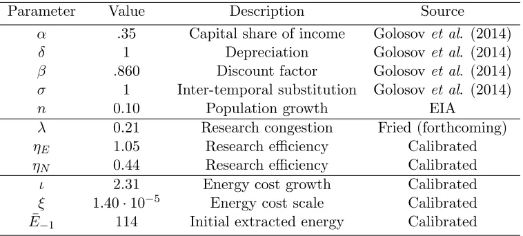
I solve the model in 10 year periods. As discussed above, the consumer and non-energy production portions of the model are standard. Thus, I take several parameters from the existing literature. In particular, I follow Golosov et al. (2014) and set α = .35, δ = 1, σ = 1, and β = .860.37 I
assume that the economy starts without environmental policy. Thus, all taxes and subsidies can be thought of as relative to ‘business as usual’ case, which serves as the baseline.
In addition to standard neoclassical elements, the putty-clay model includes R&D and energy extraction. Thus, the parameters from these segments of the model cannot be taken from the existing literature. I calibrate them to aggregate U.S. data. Data sources and details can be found in Appendix A. Due to limitations on energy expenditure data, I restrict attention to the period 1971-2014. For energy use, I use the consumption of primary energy across all sources.38
Following the structure of the model, I calculate gross output,Qt, as final output,Yt, plus energy
expenditure. I measure AE,t =Qt/Et, yielding gE∗ = 0.21 on the BGP (2.0% annual growth). On
the BGP, the growth rate of income per capita is given by g∗
R = (1 +g
∗
N) 1
1−α −1. In the data,
g∗
R= 0.19 (1.8% annual growth), which yieldsg
∗
N = 0.39. The average energy expenditure share in
the data is 8.5%, which I take to be the balanced growth level. In the data, n= 0.10.
Below, I calibrate the R&D sector of the model to match key BGP moments. The BGP is uninformative about research congestion, λ, which measures the trade-off between advances in overall productivity and energy efficiency. As a base value, I takeλ= 0.21 fromFried(forthcoming), who also captures the congestion of moving research inputs from energy-related research to general purpose research, making it a natural starting point for quantitative exercises presented here. I will also consider cases where λ∈ {0,0.105,0.31}for robustness.
36In Appendix SectionB.5, I explain the calibration procedure for Cobb-Douglas and describe the balanced growth
path. I calibrate both models so that they have identical predictions for output and energy use in the absence of environmental taxes. Due to other differences between the models, especially the difference in market structure – monopolistic competition in the putty-clay model with directed technical change and perfect competition in the Cobb-Douglas model – predictions for interest rates and levels (though not growth rates) of consumption and capital differ between the models. Given that incentives for innovation are an important part of the difference between the two models, I maintain these differences in the quantitative analysis.
37I normalize T F P
0 =E0 =L0= 10. This normalization simply sets the units of the analysis and has no effect on the quantitative results of the model. I also assume that the economy is on the BGP at timet= 0. Given the other parameters in the model, this yieldsY0= 93.50,K0= 8.25,pE,0= 0.80,AE,0= 10.15, andAN,0= 909.03.
38The model abstracts from energy transformation, implying that primary and final-use energy use are the same.