Normalized Log Linear Interpolation of Backoff Language Models is Efficient

Normalized Log-Linear Interpolation of Backoff Language Models is

Efficient

Kenneth Heafield University of Edinburgh

10 Crichton Street Edinburgh EH8 9AB

United Kingdom

[email protected]

Chase Geigle Sean Massung

University of Illinois at Urbana-Champaign 707 S. Mathews Ave.

Urbana, IL 61801 United States

{geigle1,massung1,lanes}@illinois.edu

Lane Schwartz

Abstract

We prove that log-linearly interpolated backoff language models can be efficiently and exactly collapsed into a single nor-malized backoff model, contradicting Hsu (2007). While prior work reported that log-linear interpolation yields lower per-plexity than linear interpolation, normaliz-ing at query time was impractical. We nor-malize the model offline in advance, which is efficient due to a recurrence relationship between the normalizing factors. To tune interpolation weights, we apply Newton’s method to this convex problem and show that the derivatives can be computed ef-ficiently in a batch process. These find-ings are combined in new open-source in-terpolation tool, which is distributed with KenLM. With 21 out-of-domain corpora, log-linear interpolation yields 72.58 per-plexity on TED talks, compared to 75.91 for linear interpolation.

1 Introduction

Log-linearly interpolated backoff language mod-els yielded better perplexity than linearly interpo-lated models (Klakow, 1998; Gutkin, 2000), but experiments and adoption were limited due the im-practically high cost of querying. This cost is due to normalizing to form a probability distribution by brute-force summing over the entire vocabu-lary for each query. Instead, we prove that the log-linearly interpolated model can be normalized offline in advance and exactly expressed as an or-dinary backoff language model. This contradicts Hsu (2007), who claimed that log-linearly inter-polated models “cannot be efficiently represented as a backoffn–gram model.”

We show that offline normalization is efficient due to a recurrence relationship between the

normalizing factors (Whittaker and Klakow, 2002). This forms the basis for our open-source implementation, which is part of KenLM: https://kheafield.com/code/kenlm/. Linear interpolation (Jelinek and Mercer, 1980), combines several language modelspiinto a single modelpL

pL(wn|w1n−1) = X

i

λipi(wn|wn1−1)

whereλi are weights andwn1 are words. Because each component model pi is a probability distri-bution and the non-negative weightsλi sum to1, the interpolated modelpLis also a probability dis-tribution. This presumes that the models have the same vocabulary, an issue we discuss in§3.1.

A log-linearly interpolated model pLL uses the weightsλi as powers (Klakow, 1998).

pLL(wn|w1n−1)∝ Y

i

pi(wn|w1n−1)λi

The weights λi are unconstrained real numbers, allowing parameters to soften or sharpen distribu-tions. Negative weights can be used to divide a mixed-domain model by an out-of-domain model. To form a probability distribution, the product is normalized

pLL(wn|w1n−1) = Q

ipi(wn|wn1−1)λi

Z(wn−1

1 )

where normalizing factorZ is given by

Z(wn₁−1) =X

x Y

i

pi(x|w1n−1)λi

The sum is taken over all wordsxin the combined vocabulary of the underlying models, which can number in the millions or even billions. Comput-ingZefficiently is a key contribution in this work. Our proofs assume the component modelspiare backoff language models (Katz, 1987) that mem-orize probability for seen n–grams and charge a

backoff penaltybifor unseenn–grams.

pi(wn|w1n−1) = (

pi(wn|wn1−1)ifw1nis seen

pi(wn|w₂n−1)bi(wn₁−1)o.w.

While linearly or log-linearly interpolated mod-els can be queried online by querying the compo-nent models (Stolcke, 2002; Federico et al., 2008), doing so costs RAM to store duplicatedn–grams and CPU time to perform lookups. Log-linear in-terpolation is particularly slow due to normalizing over the entire vocabulary. Instead, it is preferable to combine the models offline into a single back-off model containing the union ofn–grams. Do-ing so is impossible for linear interpolation (§3.2); SRILM (Stolcke, 2002) and MITLM (Hsu and Glass, 2008) implement an approximation. In con-trast, we prove that offline log-linear interpolation requires no such approximation.

2 Related Work

Instead of building separate models then weight-ing, Zhang and Chiang (2014) show how to train Kneser-Ney models (Kneser and Ney, 1995) on weighted data. Their work relied on prescriptive weights from domain adaptation techniques rather than tuning weights, as we do here.

Our exact normalization approach relies on the backoff structure of component models. Sev-eral approximations support genSev-eral models: ig-noring normalization (Chen et al., 1998), noise-contrastive estimation (Vaswani et al., 2013), and self-normalization (Andreas and Klein, 2015). In future work, we plan to exploit the structure of other features in high-quality unnormalized log-linear language models (Sethy et al., 2014).

Ignoring normalization is particularly common in speech recognition and machine translation. This is one of our baselines. Unnormalized mod-els can also be compiled into a single model by multiplying the weighted probabilities and back-offs.1 _{Many use unnormalized models because} weights can be jointly tuned along with other fea-ture weights. However, Haddow (2013) showed that linear interpolation weights can be jointly tuned by pairwise ranked optimization (Hopkins and May, 2011). In theory, normalized log-linear interpolation weights can be jointly tuned in the same way.

1_{Missing probabilities are found from the backoff} algo-rithm and missing backoffs are implicitly one.

Dynamic interpolation weights (Weintraub et al., 1996) give more weight to models famil-iar with a given query. Typically the weights are a function of the contexts that appear in the combined language model, which is compatible with our approach. However, normalizing factors would need to be calculated in each context. 3 Linear Interpolation

To motivate log-linear interpolation, we examine two issues with linear interpolation: normalization when component models have different vocabular-ies and offline interpolation.

3.1 Vocabulary Differences

Language models are normalized with respect to their vocabulary, including the unknown word.

X

x∈vocab(p1)

p1(x) = 1

If two models have different vocabularies, then the combined vocabulary is larger and the sum is taken over more words. Component models as-sign their unknown word probability to these new words, leading to an interpolated model that sums to more than one. An example is shown in Table 1.

p1 p2 pL Zero

<unk> 0.4 0.2 0.3 0.3

A 0.6 0.4 0.3

B 0.8 0.6 0.4

Sum 1 1 1.3 1

Table 1: Linearly interpolating two models p1 andp2 with equal weight yields an unnormalized modelpL. If gaps are filled with zeros instead, the model is normalized.

To work around this problem, SRILM (Stol-cke, 2002) uses zero probability instead of the un-known word probability for new words. This pro-duces a model that sums to one, but differs from what users might expect.

IRSTLM (Federico et al., 2008) asks the user to specify a common large vocabulary size. The un-known word probability is downweighted so that all models sum to one over the large vocabulary.

unknown word appears only as a unigram, then queries for new words will back off to unigrams. The total mass in contextw₁n−1is

1 +|new|p(<unk>)nY−1

i=1

b(w_in−1)

wherenew is the set of new words. This is effi-cient to compute online or offline. While there are tools to renormalize models, we are not aware of a tool that does this for linear interpolation.

Log-linear interpolation is normalized by con-struction. Nonetheless, in our experiments we ex-tend IRSTLM’s approach by training models with a common vocabulary size, rather than retrofitting it at query time.

3.2 Offline Linear Interpolation

Given an interpolated model, offline interpolation seeks a combined model meeting three criteria: (i) encoding the same probability distribution, (ii) be-ing a backoff model, and (iii) containbe-ing the union ofn–grams from component models.

Theorem 1. The three offline criteria cannot be satisfied for general linearly interpolated backoff models.

Proof. By counterexample. Consider the models given in Table 2 interpolated with equal weight.

p1 p2 pL

p(A) 0.4 0.2 0.3

p(B) 0.3 0.3 0.3

p(C) 0.3 0.5 0.4

p(C|A) 0.4 0.8 0.6

b(A) 6

7 ≈0.857 0.4 23 ≈0.667 Table 2: Counterexample models.

The probabilities shown forpLresult from encod-ing the same distribution. Takencod-ing the union ofn– grams implies thatpLonly has entries for A, B, C, and A C. Since the models have the same vocabu-lary, they are all normalized to one.

p(A|A) +p(B|A) +p(C|A) = 1

Since all models have backoff structure,

p(A)b(A) +p(B)b(A) +p(C|A) = 1

which when solved for backoffb(A)gives the val-ues shown in Table 2. We then query pL(B | A)

online and offline. Online interpolation yields

pL(B|A) = 1₂p1(B|A) +1₂p2(B|A)

= 1

2p1(B)b1(A) + 1

2p2(B)b2(A) = 33 175

Offline interpolation yields

pL(B|A) =pL(B)bL(A) = 0.26= ₁₇₅33 ≈0.189

The same problem happens with real language models. To understand why, we attempt to solve for the backoffbL(w1n−1). Supposingwn1 is not in either model, we querypL(wn|wn1−1)offline

pL(wn|wn−1 1)

=pL(wn|w2n−1)bL(wn−1 1)

=(λ1p1(wn|wn−2 1) +λ2p2(wn|wn−2 1))bL(w1n−1)

while online interpolation yields

pL(wn|wn−1 1)

=λ1p1(wn|wn−1 1) +λ2p2(wn|wn−1 1)

=λ1p1(wn|w2n−1)b1(wn−1 1) +λ1p2(wn|w2n−1)b2(wn−1 1)

Solving forbL(w1n−1)we obtain

λ1p1(wn|w2n−1)b1(wn−1 1) +λ2p2(wn|w2n−1)b2(wn−1 1)

λ1p1(wn|wn−2 1) +λ2p2(wn|w2n−1)

which is a weighted average of the backoff weights

b1(w1n−1) andb2(w1n−1). The weights depend on

wn, sobLis no longer a function ofwn1−1.

In the SRILM approximation (Stolcke, 2002), probabilities forn–grams that exist in the model are computed exactly. The backoff weights are chosen to produce a model that sums to one. However, newer versions of SRILM (Stolcke et al., 2011) interpolate by ingesting one component model at a time. For example, the first two mod-els are approximately interpolated before adding a third model. Ann–gram appearing only in the third model will have an approximate probabil-ity. Therefore, the output depends on the order in which users specify models. Moreover, weights were optimized for correct linear interpolation, not the approximation.

4 Offline Log-Linear Interpolation Log-linearly interpolated backoff models pi can be collapsed into a single offline modelpLL. The combined model takes the union of n–grams in component models.2 _{For thosen–grams, it} mem-orizes correct probabilitypLL.

pLL(wn|wn1−1) = Q

ipi(wn|wn1−1)λi

Z(wn₁−1) (1)

Whenwn

1 does not appear, the backoffbLL(wn1−1) modifies pLL(wn | w₂n−1) to make an appropri-ately normalized probability. To do so, it can-cels out the shorter query’s normalization term

Z(w₂n−1)then applies the correct termZ(wn₁−1). It also applies the component backoff terms.

bLL(wn1−1) = Z(w n−1

2 )

Z(wn₁−1)

Y

i

bi(wn1−1)λi (2)

Almost by construction, the model satisfies two of our criteria (§3.2): being a backoff model and containing the union ofn–grams. However, back-off models require that the backback-off weight of an unseenn–gram be implicitly1.

Lemma 1. If w₁n−1 is unseen in the combined model, then the backoff weightbLL(wn1−1) = 1.

Proof. Because we have taken the union of en-tries,wn₁−1is unseen in component models. These components are backoff models, so implicitly

bi(w1n−1) = 1∀i. Focusing on the normalization termZ(wn₁−1),

Z(wn₁−1) =X

x Y

i

pi(x|w1n−1)λi

=X

x Y

i

pi(x|w2n−1)λibi(wn1−1)λi

=X

x Y

i

pi(x|w2n−1)λi

=Z(wn−1

2 )

All of the models back off becausew₁n−1x is un-seen, being a superstring ofwn−1

1 . Relevant back-off weightsbi(w1n−1) = 1as noted earlier. Recall-ing the definition ofbLL(w1n−1),

Z(wn₂−1) Z(wn₁−1)

Y

i

bi(wn1−1)λi = Z(w n−1

2 )

Z(wn₁−1) = 1 2_{We further assume that every substring of a seenn–gram} is also seen. This follows from estimating on text, except in the case of adjusted count pruning by SRILM. In such cases, we add the missing entries to component models, with no additional memory cost in trie data structures.

We now have a backoff model containing the union ofn–grams. It remains to show that the of-fline model produces correct probabilities.

Theorem 2. The proposed offline model agrees with online log-linear interpolation.

Proof. By induction on the number of words backed off in offline interpolation. To disam-biguate, we will use pon to refer to online inter-polation andpoffto refer to offline interpolation. Base case: the queried n–gram is in the offline model and we have memorized the online prob-ability by construction.

Inductive case: Letpoff(wn | wn1−1) be a query that backs off. In online interpolation,

pon(wn|w1n−1) = Q

ipi(wn|wn1−1)λi

Z(wn−1

1 )

Becausewn

1 is unseen in the offline model and we took the union, it is unseen in every modelpi.

=

Q

ipi(wn|wn2−1)λibi(w1n−1)λi

Z(w₁n−1)

=

Q

ipi(wn|w2n−1)λi Qibi(w1n−1)λi

Z(wn₁−1)

Recognizing the unnormalized probability

Z(w₂n−1)pon(wn|wn2−1),

= Z(w2n−1)pon(wn|wn2−1)

Q

ibi(w1n−1)λi

Z(wn−1

1 )

=pon(wn|wn₂−1)Z(w n−1

2 )

Z(wn−1

1 )

Y

i

bi(wn₁−1)λi

=pon(wn|w2n−1)boff(wn1−1)

The last equality follows from the definition of

boffand Lemma 1, which extended the domain of

boff to any w1n−1. By the inductive hypothesis,

pon(wn | w2n−1) = poff(wn | wn2−1) because it backs off one less time.

=poff(wn|w2n−1)boff(w1n−1) =poff(wn|w1n−1)

The offline modelpoff(wn | w1n−1) backs off be-cause that is the case we are considering. Combin-ing our chain of equalities,

pon(wn|w1n−1) =poff(wn|w1n−1)

4.1 Normalizing Efficiently

In order to build the offline model, the normaliza-tion factorZ needs to be computed in every seen context. To do so, we extend the tree-structure method of Whittaker and Klakow (2002), which they used to compute and cache normalization fac-tors on the fly. It exploits the sparsity of language models: when summing over the vocabulary, most queries will back off. Formally, we defines(wn

1) to be the set of wordsxwherepi(x|wn1)does not back off in some model.

s(wn

1) ={x:wn1xis seen in any model} To exploit this, we use the normalizing factor

Z(wn

2)from a lower order and patch it up by sum-ming overs(wn

1).

Theorem 3. The normalization factorsZ obey a recurrence relationship:

Z(wn 1) =

X

x∈s(wn

1)

Y

i

pi(x|wn1)λi+ 

_Z(wn 2)−

X

x∈s(wn

1)

Y

i

pi(x|wn2)λi  Y

i

bi(wn1)λi

Proof. The first term handles seenn–grams while the second term handles unseen n–grams. The definition ofZ

Z(wn 1) =

X

x∈vocab Y

i

pi(x|wn1)λi

can be partitioned by cases. X

x∈s(wn

1)

Y

i

pi(x|w1n)λi+ X

x6∈s(wn

1)

Y

i

pi(x|w1n)λi

The first term agrees with the claim, so we focus on the case wherex 6∈s(wn

1). By definition ofs, all models back off.

X

x6∈s(wn

1)

Y

i

pi(x|wn1)λi

= X

x6∈s(wn

1)

Y

i

pi(x|wn2)λibi(wn1)λi

=

  X

x6∈s(wn

1)

Y

i

pi(x|wn2)λi  Y

i

bi(wn1)λi

=

 _Z(wn

2)− X

x∈s(wn

1)

Y

i

pi(x|wn2)λi  Y

i

bi(wn1)λi

This is the second term of the claim.

LM1

LM2 . . .

LM`

Merge probabilities (§4.2.1)

Apply Backoffs (§4.2.2)

Normalize (§4.2.3)

Output (§4.2.4) Context sort *_wn

1_Q, m(w1n), +

ipi(wn|wmn−i(1w1n))

λi),

Q

ipi(wn|w_mn−_i(1_wn

2))

λi)

In context order *_wn

1,_QQibi(wn1−1)λi, + ipi(wn|wn1−1)λi, Q

ipi(wn|wn2−1)λi

In suffix order

bLL(wn1)

Suffix sort *

wn

1, pLL(wn|wn1−1) +

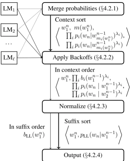
Figure 1: Multi-stage streaming pipeline for of-fline log-linear interpolation. Bold arrows indicate sorting is performed.

The recurrence structure of the normalization factors suggests a computational strategy: com-puteZ()by summing over the unigrams,Z(wn) by summing over bigramswnx,Z(wnn−1)by sum-ming over trigramswn

n−1x, and so on.

4.2 Streaming Computation

Part of the point of offline interpolation is that there may not be enough RAM to fit all the com-ponent models. Moreover, with compression tech-niques that rely on immutable models (Whittaker and Raj, 2001; Talbot and Osborne, 2007), a mu-table version of the combined model may not fit in RAM. Instead, we construct the offline model with disk-based streaming algorithms, using the frame-work we designed for language model estimation (Heafield et al., 2013). Our pipeline (Figure 1) has four conceptual steps: merge probabilities, apply backoffs, normalize, and output. Applying back-offs and normalization are performed in the same pass, so there are three total passes.

4.2.1 Merge Probabilities

assume that the component models are sorted in suffix order (Figure 4), which is true of models produced by lmplz (Heafield et al., 2013) or stored in a reverse trie. Moreover, despite having different word indices, the models are consistently sorted using the string word, or a hash thereof.

3 2 1

A A A A A A B A A B

Table 3: Merging probabilities processesn–grams in lexicographic order by suffix. Column headings indicate precedence.

The algorithm processes n–grams in lexico-graphic (depth-first) order by suffix (Table 3). In this way, the algorithm processespi(A) before it might be used as a backoff point for pi(A | B) in one of the models. It jointly streams through all models, so thatp1(A|B)andp2(A|B)are avail-able at the same time. Ideally, we would compute unnormalized probabilities.

Y

i

pi(wn|wn1−1)λi

However, these queries back off when models con-tain different n–grams. The appropriate backoff weights bi(wn1−1) are not available in a stream-ing fashion. Instead, we proceed without chargstream-ing backoffs

Y

i

pi(wn|wn_m−_i(1_wn

1))

λi

where mi(w1n) records what backoffs should be charged later.

The normalization step (§4.2.3) also uses lower-order probabilities

Y

i

pi(wn|wn₂−1)λi

and needs to access them in a streaming fashion, so we also output

Y

i

pi(wn|wn_m−_i(1_wn

2))

λi

Suffix

3 2 1

Z B A Z A B B B B

Context

2 1 3

Z A B B B B Z B A

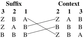
Table 4: Sorting orders (Heafield et al., 2013). In suffix order, the last word is primary. In context order, the penultimate word is primary. Column headings indicate precedence.

Each output tuple has the form *

wn₁, m(w₁n),Y

i

pi(wn|w_mn−_i(1_wn

1))

λi_,

Y

i

pi(wn|w_mn−_i(1_wn

2))

λi

+

wherem(wn

1)is a vector of backoff requests, from whichm(wn

2)can be computed.

4.2.2 Apply Backoffs

This step fulfills the backoff requests from merg-ing probabilities. The merged probabilities are sorted in context order (Table 4) so that n– grams wn

1 sharing the same context wn1−1 are consecutive. Moreover, contexts wn−1

1 appear in suffix order. We use this property to stream through the component models again in their native suffix order, this time reading backoff weightsbi(wn1−1), bi(w2n−1), . . . , bi(wn−1). Mul-tiplying the appropriate backoff weights by Q

ipi(wn|w_mn−_i(1_wn

1))

λi yields unnormalized

proba-bility _Y

i

pi(wn|w₁n−1)λi

The same applies to the lower order. Y

i

pi(wn|w2n−1)λi

This step also merges backoffs from component models, with output still in context order.

*

wn₁,Y

i

bi(wn₁−1)λi, Y

i

pi(wn|wn₁−1)λi

Y

i

pi(wn|wn2−1)λi +

4.2.3 Normalize

This step computes normalization factor Z for all contexts, which it applies to produce pLL and

bLL. Recalling§4.1,Z(w₁n−1)is efficient to com-pute in a batch process by processing suffixes

Z(), Z(wn), . . . Z(wn2−1) first. In order to min-imize memory consumption, we chose to evaluate the contexts in depth-first order by suffix, so that

Z(A)is computed immediately before it is needed to computeZ(A A)and forgotten atZ(B).

Computing Z(w₁n−1) by applying Theorem 3 requires the sum

X

x∈s(w₁n−1) Y

i

pi(x|w₁n−1)λi

wheres(wn−1

1 )restricts to seenn–grams. For this, we stream through the output of the apply backoffs step in context order, which makes the various val-ues of xconsecutive. Theorem 3 also requires a sum over the lower-order unnormalized

probabili-ties _X

x∈s(wn−1 1 )

Y

i

pi(x|w2n−1)λi

We placed these terms in the input tuple for

wn₁−1x. Otherwise, it would be hard to access these values while streaming in context order.

While we have shown how to compute

Z(w₁n−1), we still need to normalize the probabil-ities. Unfortunately,Z(wn₁−1)is only known after streaming through all records of the formwn−1

1 x, which are the very same records to normalize. We therefore buffer up to the vocabulary size for each order in memory to allow rewinding. Processing contextwn₁−1thus yields normalized probabilities

pLL(x|wn1−1)for all seenwn1−1x. D

wn

1, pLL(x|w1n−1) E

These records are generated in context order, the same order as the input.

The normalization step also computes backoffs.

bLL(w1n−1) = Z(w n−1

2 )

Z(wn₁−1)

Y

i

bi(w1n−1)λi

NormalizationZ(w₁n−1)is computed by this step, numeratorZ(wn−1

2 )is available due to depth-first search, and the backoff terms Q_ibi(w1n−1)λi are present in the input. The backoffsbLL are gener-ated in suffix order, since each context produces a backoff value. These are written to a sidechannel stream as bare values without keys.

4.2.4 Output

Language model toolkits store probability

pLL(wn|w1n−1)and backoffbLL(wn1)together as values for the key wn

1. To reunify them, we sort

hwn

1, pLL(wn | w1n−1)i in suffix order and merge with the backoff sidechannel from normalization, which is already in suffix order. Suffix order is also preferable because toolkits can easily build a reverse trie data structure.

5 Tuning

Weights are tuned to maximize the log probability of held-out data. This is a convex optimization problem (Klakow, 1998). Iterations are expensive due to the need to normalize over the vocabulary at least once. However, the number of weights is small, which makes the Hessian matrix cheap to store and invert. We therefore selected Newton’s method.3

The log probability of tuning datawis

logY

n

pLL(wn|w1n−1)

which expands according to the definition ofpLL X

n X

i

λilogpi(wn|wn₁−1) !

−logZ(w₁n−1)

The gradient with respect toλihas a compact form X

n

logpi(wn|wn1−1) +CH(pLL, pi |wn1−1)

where CH is cross entropy. However, comput-ing the cross entropy directly would entail a sum over the vocabulary for every word in the tun-ing data. Instead, we apply Theorem 3 to ex-pressZ(wn−1

1 ) in terms of Z(w2n−1) before tak-ing the derivative. This allows us to perform the same depth-first computation as before (§4.2.3), only this time ∂

∂λiZ(w

n−1

1 )is computed in terms of ∂

∂λiZ(w

n−1 2 ).

The same argument applies when taking the Hessian with respect to λi and λj. Rather than compute it directly in the form

X

n

−X

x

pLL(x|wn−1

1 ) logpi(x|wn−1 1) logpj(x|w1n−1)

+CH(pLL, pi|w1n−1)CH(pLL, pj|wn−1 1)

we apply Theorem 3 to compute the Hessian for

wn

1 in terms of the Hessian forw2n.

6 Experiments

We perform experiments for perplexity, query speed, memory consumption, and effectiveness in a machine translation system.

Individual language models were trained on En-glish corpora from the WMT 2016 news transla-tion shared task (Bojar et al., 2016). This includes the seven newswires (afp, apw, cna, ltw, nyt, wpb, xin) from English Gigaword Fifth Edition (Parker et al., 2011); the 2007–2015 news crawls;4 News discussion; News commmentary v11; En-glish from Europarl v8 (Koehn, 2005); the EnEn-glish side of the French-English parallel corpus (Bojar et al., 2013); and the English side of SETIMES2 (Tiedemann, 2009). We additionally built one lan-guage model trained on the concatenation of all of the above corpora. All corpora were prepro-cessed using the standard Moses (Koehn et al., 2007) scripts to perform normalization, tokeniza-tion, and truecasing. To prevent SRILM from run-ning out of RAM, we excluded the large mono-lingual CommonCrawl data, but included English from the parallel CommonCrawl data.

All language models are 5-gram backoff lan-guage models trained with modified Kneser-Ney smoothing (Chen and Goodman, 1998) using lmplz (Heafield et al., 2013). Also to prevent SRILM from running out of RAM, we pruned sin-gleton trigrams and above.

For linear interpolation, we tuned weights us-ing IRSTLM. To work around SRILM’s limitation of ten models, we interpolated the first ten then carried the combined model and added nine more component models, repeating this last step as nec-essary. Weights were normalized within batches to achieve the correct final weighting. This simply extends the way SRILM internally carries a com-bined model and adds one model at a time.

6.1 Perplexity experiments

We experiment with two domains: TED talks, which is out of domain, and news, which is in-domain for some corpora. For TED, we tuned on the IWSLT 2010 English dev set and test on the 2010 test set. For news, we tuned on the English side of the WMT 2015 Russian–English evaluation set and test on the WMT 2014 Russian– English evaluation set. To measure generalization, we also evaluated news on models tuned for TED and vice-versa. Results are shown in Table 5.

4_{For News Crawl 2014, we used version 2.}

Component Models Component TED test News test

Gigaword afp 163.48 221.57 Gigaword apw 140.65 206.85 Gigaword cna 299.93 448.56 Gigaword ltw 106.28 243.35

Gigaword nyt 97.21 211.75

Gigaword wpb 151.81 341.48 Gigaword xin 204.60 246.32

News 07 127.66 243.53

News 08 112.48 202.86

News 09 111.43 197.32

News 10 114.40 209.31

News 11 107.69 187.65

News 12 105.74 180.28

News 13 104.09 155.89

News 14 v2 101.85 139.94

News 15 101.13 141.13

News discussion 99.88 249.63 News commentary v11 236.23 495.27

Europarl v8 268.41 574.74

CommonCrawl fr-en.en 149.10 343.20 SETIMES2 ro-en.en 331.37 521.19 All concatenated 80.69 96.15

TED weights Interpolation TED test News test

Offline linear 75.91 100.43 Online linear 76.93 152.37

Log-linear 72.58 112.31

News weights Interpolation TED test News test

Offline linear 83.34 107.69 Online linear 83.94 110.95

Log-linear 89.62 124.63

LM Tuning Compiling Querying

All concatenated N/A N/A N/A N/A 0.186µs 46.7G Offline linear 0.876m 60.2G 641m 123G 0.186µs 46.8G Online linear 0.876m 60.2G N/A N/A 5.67µs 89.1G Log-linear 600m 63.9G 89.8m 63.9G 0.186µs 46.8G

Table 6: Speed and memory consumption of LM combination methods. Interpolated models include the concatenated model. Tuning and compiling times are in minutes, memory consumption in gigabytes, and query time in microseconds per query (on 1G of held-out Common Crawl monolingual data).

Log-linear interpolation performs better on TED (72.58 perplexity versus 75.91 for offline lin-ear interpolation). However, it performs worse on news. In future work, we plan to investigate whether log-linear wins when all corpora are out-of-domain since it favors agreement by all models. Table 6 compares the speed and memory per-formance of the competing methods. While the log-linear tuning is much slower, its compilation is faster compared to the offline linear model’s long run time. Since the model formats are the same for the concatenation and log-linear, they share the fastest query speeds. Query speed was mea-sured using KenLM’s (Heafield, 2011) faster prob-ing data structure.5

6.2 MT experiments

We trained a statistical phrase-based machine translation system for Romanian-English on the Romanian-English parallel corpora released as part of the 2016 WMT news translation shared task. We trained three variants of this MT system. The first used a single language model trained on the concatenation of the 21 individual LM train-ing corpora. The second used 22 language mod-els, with each LM presented to Moses as a sep-arate feature. The third used a single language model which is an interpolation of all 22 mod-els. This variant was run with offline linear, online linear, and log-linear interpolation. All MT sys-tem variants were optimized using IWSLT 2011 Romanian-English TED test as the development set, and were evaluated using the IWSLT 2012 Romanian-English TED test set.

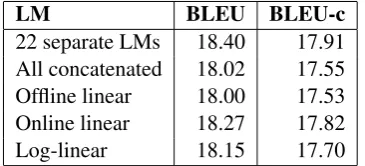
As shown in Table 7, no significant difference in MT quality as measured by BLEU was observed; the best BLEU score came from separate features at18.40while log-linear scored18.15. We leave

5_{KenLM does not natively implement online linear} inter-polation, so we wrote a custom wrapper, which is faster than querying IRSTLM.

LM BLEU BLEU-c

22 separate LMs 18.40 17.91 All concatenated 18.02 17.55 Offline linear 18.00 17.53 Online linear 18.27 17.82 Log-linear 18.15 17.70 Table 7: Machine translation performance com-parison in an end-to-end system.

jointly tuned normalized log-linear interpolation to future work.

7 Conclusion

Normalized log-linear interpolation is now a tractable alternative to linear interpolation for backoff language models. Contrary to Hsu (2007), we proved that these models can be exactly col-lapsed into a single backoff language model. This solves the query speed problem. Empiri-cally, compiling the log-linear model is faster than SRILM can collapse its approximate offline linear model. In future work, we plan to improve per-formace of feature weight tuning and investigate more general features.

Acknowledgments

Thanks to Jo˜ao Sedoc, Grant Erdmann, Jeremy Gwinnup, Marcin Junczys-Dowmunt, Chris Dyer, Jon Clark, and MT Marathon attendees for discus-sions. Partial funding was provided by the Ama-zon Academic Research Awards program. This material is based upon work supported by the NSF GRFP under Grant Number DGE-1144245.

References

Ondˇrej Bojar, Christian Buck, Chris Callison-Burch, Christian Federmann, Barry Haddow, Philipp Koehn, Christof Monz, Matt Post, Radu Soricut, and Lucia Specia. 2013. Findings of the 2013 workshop on statistical machine translation. InProceedings of the Eighth Workshop on Statistical Machine Trans-lation, pages 1–44, Sofia, Bulgaria, August. Associ-ation for ComputAssoci-ational Linguistics.

Ondˇrej Bojar, Christian Buck, Rajen Chatterjee, Chris-tian Federmann, Liane Guillou, Barry Haddow, Matthias Huck, Antonio Jimeno Yepes, Aur´elie N´ev´eol, Mariana Neves, Pavel Pecina, Martin Popel, Philipp Koehn, Christof Monz, Matteo Negri, Matt Post, Lucia Specia, Karin Verspoor, J¨org Tiede-mann, and Marco Turchi. 2016. Findings of the 2016 Conference on Machine Translation. In Pro-ceedings of the First Conference on Machine Trans-lation (WMT’16), Berlin, Germany, August. Stanley Chen and Joshua Goodman. 1998. An

em-pirical study of smoothing techniques for language modeling. Technical Report TR-10-98, Harvard University, August.

Stanley F. Chen, Kristie Seymore, and Ronald Rosen-feld. 1998. Topic adaptation for language modeling using unnormalized exponential models. In Acous-tics, Speech and Signal Processing, 1998. Proceed-ings of the 1998 IEEE International Conference on, volume 2, pages 681–684. IEEE.

Marcello Federico, Nicola Bertoldi, and Mauro Cet-tolo. 2008. IRSTLM: an open source toolkit for handling large scale language models. In Proceed-ings of Interspeech, Brisbane, Australia.

Alexander Gutkin. 2000. Log-linear interpolation of language models. Master’s thesis, University of Cambridge, November.

Barry Haddow. 2013. Applying pairwise ranked opti-misation to improve the interpolation of translation models. InProceedings of NAACL.

Kenneth Heafield, Ivan Pouzyrevsky, Jonathan H. Clark, and Philipp Koehn. 2013. Scalable modi-fied Kneser-Ney language model estimation. In Pro-ceedings of the 51st Annual Meeting of the Associa-tion for ComputaAssocia-tional Linguistics, Sofia, Bulgaria, August.

Kenneth Heafield. 2011. KenLM: Faster and smaller language model queries. InProceedings of the Sixth Workshop on Statistical Machine Translation, Edin-burgh, UK, July. Association for Computational Lin-guistics.

Mark Hopkins and Jonathan May. 2011. Tuning as ranking. InProceedings of the 2011 Conference on Empirical Methods in Natural Language Process-ing, pages 1352—-1362, Edinburgh, Scotland, July. Bo-June Hsu and James Glass. 2008. Iterative lan-guage model estimation: Efficient data structure & algorithms. In Proceedings of Interspeech, Bris-bane, Australia.

Bo-June Hsu. 2007. Generalized linear interpolation of language models. InAutomatic Speech Recogni-tion & Understanding, 2007. ASRU. IEEE Workshop on, pages 136–140. IEEE.

Frederick Jelinek and Robert L. Mercer. 1980. In-terpolated estimation of Markov source parameters from sparse data. In Proceedings of the Workshop on Pattern Recognition in Practice, pages 381–397, May.

Slava Katz. 1987. Estimation of probabilities from sparse data for the language model component of a speech recognizer. IEEE Transactions on Acoustics, Speech, and Signal Processing, ASSP-35(3):400– 401, March.

Dietrich Klakow. 1998. Log-linear interpolation of language models. In Proceedings of 5th Interna-tional Conference on Spoken Language Processing, pages 1695–1699, Sydney, November.

Reinhard Kneser and Hermann Ney. 1995. Improved backing-off for m-gram language modeling. In Proceedings of the IEEE International Conference on Acoustics, Speech and Signal Processing, pages 181–184.

Philipp Koehn, Hieu Hoang, Alexandra Birch, Chris Callison-Burch, Marcello Federico, Nicola Bertoldi, Brooke Cowan, Wade Shen, Christine Moran, Richard Zens, Chris Dyer, Ondˇrej Bojar, Alexan-dra Constantin, and Evan Herbst. 2007. Moses: Open source toolkit for statistical machine transla-tion. InAnnual Meeting of the Association for Com-putational Linguistics (ACL), Prague, Czech Repub-lic, June.

Philipp Koehn. 2005. Europarl: A parallel corpus for statistical machine translation. In Proceedings of MT Summit.

Robert Parker, David Graff, Junbo Kong, Ke Chen, and Kazuaki Maeda. 2011. English gigaword fifth edi-tion, June. LDC2011T07.

Abhinav Sethy, Stanley Chen, Bhuvana Ramabhadran, and Paul Vozila. 2014. Static interpolation of ex-ponentialn–gram models using features of features. In2014 IEEE International Conference on Acoustic, Speech and Signal Processing (ICASSP).

Andreas Stolcke, Jing Zheng, Wen Wang, and Vic-tor Abrash. 2011. SRILM at sixteen: Update and outlook. In Proc. 2011 IEEE Workshop on Automatic Speech Recognition & Understanding (ASRU), Waikoloa, Hawaii, USA.

Andreas Stolcke. 2002. SRILM - an extensible lan-guage modeling toolkit. InProceedings of the Sev-enth International Conference on Spoken Language Processing, pages 901–904.

J¨org Tiedemann. 2009. News from OPUS - A col-lection of multilingual parallel corpora with tools and interfaces. In N. Nicolov, K. Bontcheva, G. Angelova, and R. Mitkov, editors, Recent Advances in Natural Language Processing, vol-ume V, pages 237–248. John Benjamins, Amster-dam/Philadelphia, Borovets, Bulgaria.

Ashish Vaswani, Yinggong Zhao, Victoria Fossum, and David Chiang. 2013. Decoding with large-scale neural language models improves translation. In Proceedings of EMNLP.

Mitch Weintraub, Yaman Aksu, Satya Dharanipragada, Sanjeev Khudanpur, Hermann Ney, John Prange, Andreas Stolcke, Fred Jelinek, and Liz Shriberg. 1996. LM95 project report: Fast training and portability. Research Note 1, Center for Language and Speech Processing, Johns Hopkins University, February.

Edward D. W. Whittaker and Dietrich Klakow. 2002. Efficient construction of long-range language mod-els using log-linear interpolation. In 7th Interna-tional Conference on Spoken Language Processing, pages 905–908.

Edward Whittaker and Bhiksha Raj. 2001. Quantization-based language model compres-sion. InProceedings of Eurospeech, pages 33–36, Aalborg, Denmark, December.