University of Warwick institutional repository: http://go.warwick.ac.uk/wrap
This paper is made available online in accordance with
publisher policies. Please scroll down to view the document
itself. Please refer to the repository record for this item and our
policy information available from the repository home page for
further information.
To see the final version of this paper please visit the publisher’s website
.
Access to the published version may require a subscription.
Author(s): Y Pokern, O Papaspiliopoulos, GO Roberts and AM Stuart
Article Title: Non parametric Bayesian drift estimation for
one-dimensional diffusion processes
Year of publication: 2009
Link to published article:
http://www2.warwick.ac.uk/fac/sci/statistics/crism/research/2009/paper
09-29
NONPARAMETRIC BAYESIAN DRIFT ESTIMATION FOR ONE-DIMENSIONAL DIFFUSION PROCESSES
By Yvo Pokern∗, Omiros Papaspiliopoulos†, Gareth O.
Roberts∗ and Andrew M. Stuart‡
We consider diffusions on the circle and establish a Bayesian esti-mator for the drift function based on observing the local time and us-ing Gaussian priors. Given a standard Girsanov likelihood, we prove that the procedure is well-defined and that the posterior enjoys ro-bustness against small deviations of the local time. A simple method for estimating the local time from high-frequency discrete time obser-vations yielding control of the L2 error is proposed. Complemented by a finite element implementation this enables error-control for a fixed random sample all the way from high-frequency discrete ob-servation to the numerical computation of the posterior mean and covariance. An empirical Bayes procedure is suggested which allows automatic selection of the smoothness of the prior in a given family. Some numerical experiments extend our observations to subsets of the real line other than circles and exhibit more probabilistic conver-gence properties such as rates of posterior contraction.
1. Introduction.
1.1. Setup. This paper considers non-parametric estimation of drift func-tionalsb(·) in one-dimensional Itˆo stochastic differential equations with con-stant diffusivity such as
(1) dx=b(x)dt+dB, x(0) =x0.
Here,Brefers to a standard Brownian motion andb(·) is the drift functional to be estimated, with anti-derivative denoted as V′ =b. We shall consider
the case where observations ofx are available continuously on a finite time interval, and describe numerical methods to approximate to this ideal in the case where we have high-frequency observations.
Maximum likelihood estimation for this problem turns out to be ill-posed, and thus a Bayesian approach is natural, in which we can use priors which impose suitable smoothness onbso that the supports of prior and posterior distributions are sufficiently well-behaved. For technical reasons, we assume
∗Department of Statistics, University of Warwick, Coventry, U.K. †Department of Economics, Universitat Pompeu Fabra, Barcelona, Spain ‡Mathematics Institute, University of Warwick, Coventry, U.K.
periodic boundary conditions on the prior forb, i.e. the SDE has the circle as a state space, which we parametrize by the interval [0,2π] with suitable identification of the end points. The compactness this provides offers most welcome simplifications of the proofs later. In the numerical part of the paper, we will exhibit how our methodology can be extended to bounded and unbounded intervals on the real line as state spaces.
1.2. Likelihood. To see why the likelihood we employ for our framework is reasonable, denote the measure on path spaceC([0, T],[0,2π]) induced by Brownian motion on the circle as Q. Similarly, denote the measure on the same space induced by (1) as Pb. Then the Girsanov change of measure is given as
(2) dPb
dQ = exp (−I[b])
where the functionalI[b] is given as follows:
I[b] = 1 2
Z T
0 |
b(xt)|2dt−
Z T
0
b(xt)dxt. (3)
We now use Itˆo’s formula for dV to eliminate the stochastic integral:
I[b] = 1 2
Z T
0
|b(xt)|2+b′(xt)
dt−V(xT) +V(x0)−W(V(2π)−V(0)), where we use W to denote the (signed) number of times the path wraps around the circle. Clearly, the winding numberW is without influence when-ever the potential V (and not just the drift function b) is periodic.
For statistical interpretation, it is natural to want to replace the time integral in (3) by a space integral in order to easily assess the piecewise in-fluence of the likelihood onb. To this end, recall the local time of a stochastic process:
LT(a) = lim ǫ→0
1 2ǫ
Z T
0
1(a−ǫ,a+ǫ)(xs)ds ,
IfLT(·) were differentiable, it would then be possible to rewrite (3) as
I[b] = 1 2
Z 2π
0
|b(a)|2+b′(a)LT(a)da−V(xT) +V(x0)−W(V(2π)−V(0)) = 1
2
Z 2π
0
h
|b(a)|2LT(a)−b(a)L′T(a)−2b(a) (W + ˜χ(a;X0, XT))
i da
˜
χ(a;X0, XT) =
1 ifX0 < a < XT −1 ifXT < a < X0
0 otherwise
.
We aim to adopt the expression (4) as our log-likelihood. However unfor-tunately LT is almost surely not differentiable at any point, so one of the complications of our approach will be to make clear mathematical sense out of this representation.
1.3. Heuristic Bayesian Calculation. To complete the Bayesian frame-work, a prior and resulting posterior measure are needed and it turns out that families of Gaussian processes
b∼ N(b0,A−1)
with meanb0 and precision operator Adefined on a suitable function space
H that takes periodicity into account are naturally conjugate within our context. In a first pass, we present heuristic calculations only which we will make rigorous in subsequent sections. We start by writing the Gaussian measure as a density with respect to (non-existing) Lebesgue measure on
H:
(5) p0(b)∝exp
−1 2
Z 2π
0 (b−b0)(a)(A(b−b0))(a)da
Given an observation of a sample path xt in continuous time, Bayes for-mula then yields the following formal density for the posterior measure:
Pb|{xt}Tt=0
∝P({xt}t=0T |b)p0(b) = exp
−1 2
Z 2π
0
Lb2−bL′−2b(W + ˜χ(·;X0, XT))da
−1 2
Z 2π
0 (b−b0)A(b−b0)da
Completing the square in the exponent one finds that this is again a Gaussian with Mean
(6) bb= (A+LT)−1
1
2L
′
T +W + ˜χ(·;X0, XT) +Ab0
and covariance
(7) Co= (A+LT)−1,
where we abbreviate the informative part of the right hand side in (¡refeq:gaussMean) to f for future use:
f = 1
2L
′
T +W + ˜χ(·;X0, XT)
Prior Elicitation. The conditional independence structure of the prior (and by inheritance the posterior) is specified infinitesimally through the operator A, and this in turn determines the prior smoothness imposed on the functionb. There is considerable latitude in choosing theA, though we shall restrict ourselves to the consideration of priors with precision operators of the form
A=η∆k+ǫ
(8)
forη >0,ǫ≥0 andk∈ {1,2}, where the Laplace operator ∆ is simply the second derivative in this one-dimensional case: ∆ = dad22. The effect of the hyperparameters will be to enforce smoothness or low variability for large values ofη, whereas large values ofǫimpose a stronger bias towards the con-stant zero function. The hyperparameterk affects the regularity of samples from prior and posterior measure which are in the Sobolev class,Hk−12−εfor any ε >0 (in any case, the SDE (1) still needs to make sense when using a typical sample from (5), see Subsection 5.0.2). So the choicek= 1 results in samples from the posterior which enjoy Brownian regularity, whereask= 2 leads to the same regularity as that of integrated Brownian motion. This choice of precision operator not only results in familiar regularity but also in a Markovian structure so that it is possible to think of samples from the posterior as realizations of Brownian motion or its integral. Other, higher integer as well as fractional powers of ∆ could be considered but are more cumbersome to implement for the discretisation methods considered.
The heuristic Bayesian calculations are made rigorous for the caseη=ǫ= 1 withk= 2 but this will carry over to anyǫ >0, η >0 in a straightforward manner. We also perform numerical experiments in the cases of k= 1 and
ǫ= 0.
the analysis and, secondly, Robin boundary conditions are seen to arise from Gaussian (instead of periodic) boundary conditions. The Gaussian boundary conditions allow us to conceive of draws from the prior measure as realiza-tions of the Brownian bridge with start and end points drawn independently from a Gaussian distribution. Draws from the posterior measure share the properties concerning the end points and could possibly be thought of as draws from a conditioned SDE.
While this subsection is mostly formal we believe that much of the analysis in the sequel could be made rigorous but renounce a complete exposition along the lines of the analysis presented in this paper for the sake of brevity.
Formal Calculation. In this paragraph, we construct a new prior measure implementing Gaussian boundary conditions. Consider multiplying another Gaussian density,
bboundary∼exp
−21σ2b2(y)− 1 2σ2b
2(z)
for the beginning and end points,y and z, with the improper prior ˜
µ0 =N(0,∆−1)⊕λ
where the Gaussian measure lives on ˙L2(y, z), the space of square integrable functions on (y, z) with average zero and we use Lebesgue measure on the space{a1:a∈R}of constant functions.
We assume that the pointsy and z have been chosen such that the local time LT is informative on [y, z] but nearly zero outside. It then turns out that this translates into a Robin boundary condition for the PDE for the posterior mean, which we demonstrate in the following formal calculation for the posterior probabilityµ(b):
I[b] =−log(P(b|LT,prior)) (9)
= 1 2
Z z
y
η(b′)2(a) +LT(a)b2(a)−b(a)L′T(a)−2b(a) ˜χ(a;X0, XT)da (10)
+ 1 2σ2b
2(y) + 1 2σ2b
2(z) + const (11)
To find a critical point of this functional, take its variation for small devia-tionsεv from band perform a partial integration:
I[b+εv]−I[b] =ε
Z z
y
ηb′v′+LTbv− 1
2vLT −vχda˜ +b(y)v(y) +b(z)v(z)
Now perform a partial integration in the first integral to find that the new PDE to be solved reads
−ηb′′+LTb= 1 2L
′
T + ˜χ, b(y) =σ2ηb′(y), b(z) =σ2ηb′(z) (12)
The new boundary condition relating the value of the function at the bound-ary to the value of its derivative is known as a Robin boundbound-ary condition.
1.5. Estimating Smoothness Hyperparameters. It is possible to employ an empirical Bayes framework, where the constants η and ǫ in the prior (8) are treated as hyperparameters taking values in (0,∞)×[0,∞). As the numerical experiments will highlight, performance of the estimator depends on the value of these constants, and while it is possible to extend to a hierarchical prior, we will simply employ maximization of the integration constant P({xt}Tt=0), i.e. we will require
η = arg max η∈(0,∞),ǫ∈[0,∞)
Z
L2P({xt}
T
t=0|b)p0(db)
leaving the order parameterkfixed. The integral can be computed formally again by completing the square and turns out to be
Z
L2P({xt}
T
t=0|b)p0(db) =
q
|Id +A−1(η, ǫ)L T|−1 · (13)
exp
−1 2
Z 2π
0
h
−(A(η, ǫ)b0+f) (A(η, ǫ) +LT)−1(A(η, ǫ)b0+f) +b0A(η, ǫ)b0
i da
.
Although this computation is entirely formal, it is possible to evaluate the resulting expression numerically and investigate robustness of the results un-der refinement of resolution. It should be noted that there are no guarantees that a maximizer will exist in the specified region (η, ǫ) ∈ (0,∞)×[0,∞), and we observe that, in fact, for some datasets, the maximum is attained at the boundary, while for other datasets reasonable and robust valuesη,b bǫare obtained, as will be seen in Section 3.2.
1.6. Overview of the Paper. In the remaining sections we rigorously es-tablish the Bayesian framework presented above and report numerical ex-periments highlighting the performance of these estimators, possibilities for tuning and a practical application.
in Section 4 to make the point that our method is practically usable. The mathematical detail is tackled in Sections 5 to 8. We proceed by first establishing existence and support of the prior measure in Section 5.
In order to approach the posterior measure we simply define a Gaussian measure with the mean and covariance suggested by (7) and then proceed to show that this definition satisfies all requirements of the posterior measure. In detail, we study the PDE relating prior and posterior means in Section 6 showing that the posterior mean is well-defined as the unique weak solution of the PDE (6). We continue by establishing existence and absolute conti-nuity of posterior to prior measure in Section 7 and we verify (subject to a technical assumption) that the Radon-Nikodym derivative is in fact given by the likelihood (2) above.
It may be more natural to simply define the posterior measure as the product of the prior measure and the likelihood, however we have found it difficult to make our calculations rigorous using that approach.
We give a brief description of a simple method to estimate the local time from discrete high frequency observations in Section 8 but have to stress that this assumes adaptation of the spatial resolution to the observed time series.
Finally, in Section 9, we discuss natural extensions of this work.
non-parametric density estimation with striking similarities in the kind of prior and posterior measures used in [14]. Also, our work is motivated in part by known connections between between penalized nonparametric regression and Bayesian inference using Gaussian process priors, see [?].
This is in sharp contrast with the vast literature on Bayesian parametric inference for diffusion processes; for methodological work in this direction see for example [18], [17], [4], and for theoretical properties of Bayes estimators see for example [12] and [5].
2. Finite Element Implementation. In this section we briefly show an implementation of our estimator based on a finite element discretisation of the equations (6) and (7). For the sake of brevity we do not give details but follow standard practice in numerical analysis and provide pointers to the relevant literature. First though we shall briefly describe some essential mathematical preliminaries.
2.1. Finite Elements.
2.1.1. Function Spaces. Before defining the prior measure, we introduce notation for Sobolev spaces used in the definition as well as throughout the paper. We use the Sobolev spacesHs(U) (fors∈NandU an open bounded subset of someRn) of square integrable functions withsweak, square inte-grable derivatives with the inner product (·,·)Hs and induced normk · kHs. We denote the separable Hilbert subspace of functions with average zero by
˙
Hs(U). Furthermore, it is possible to impose periodic boundary conditions for Sobolev spaces of high enough order and we denote the Sobolev space of periodic functions on the interval (a, b) by Hs
per(a, b) for s≥1.
A convenient summary of Sobolev space fundamentals especially for the periodic case is given in [21] with a fuller treatment available from [11], whereas [2] contains a comprehensive treatment of this rich area. See also the neat treatment of weak solutions in [8].
We choose a Hilbert-subspace Hh2 of H2 to discretize and implement the above estimator, in particular solving equations (6) and (7) respectively.Hh2
is just defined as the subset ofH2consisting of cubic splines with continuous first derivatives, see Section 3.4.3 of [19] for details.
The fact thatHh2⊂H2 is referred to as usingconforming finite elements and for H2 in 1-dimension, piecewise cubic polynomials are the minimal requirement. Their regularity is sufficient by Theorem 5.2 in [7] and we employ these elements are recommended in [15] as well as [19].
We thus represent functions u ∈ H2
h
Local time is discretised using a histogram withB bins and piecewise con-stant (P0) functions leading to a natural discretisation of the linear form
φ(u) =R02πu′(a)L(a)da. The trilinear formψ(u, L, v) =R2π
0 u(a)L(a)v(a)da is also straightforward to discretize, somewhat akin to standard mixed finite element discretizations of the trilinear form in the Navier Stokes equation, see e.g. Chapter III.5 in [7] in the context of the Stokes equation.
Exploiting the coercivity shown in Lemma 1 in the appendix, Section 10.2, it is then possible to show that the solutions to the discretised system are only O(h) away in H2-norm from the true solution, using the general version of C´ea’s Lemma from [15]. This type of result is often stated as the error of approximation being bounded above by the error of interpolation:
Theorem 1. Let u be the true solution of (6) with η = ǫ = 1, k = 2
and periodic boundary conditions (formally described in (30)) and letuh be
the spline function in H2
h corresponding to the solution U of the discretised
problem
S2U +M U+MLU =M(W + ˜χh(·;X0, XT)) +CLT,h (14)
where S2, M and ML are matrices arising from suitable finite element
dis-cretizations of the differential operator ∆2 and the multiplication operators
I and LT ·I respectively, then we have the bound
ku−uhkH2 ≤
C α vhinf∈H2h
ku−vhkH2, (15)
where the constantsαandCare the constants of coercivity and of continuity as in Lemma 1.
To bound the error of interpolation, we refer to [19], Section 3.4.3. 3. Experimental results.
3.1. Setup. As a concrete example we study the SDE (16) dx=−sin(x) + 3 cos2(x) sin(x)dt+dB, x(0) = 2
3π
The Exact Algorithm 1 from [1] is used to generate a sample path for final timeT = 2000. The resolution timestep is δt= 0.001 and only the samples at time points {jδt}2·106
the local time (i.e. potential intermediate skeleton points are discarded). For the portions of that path obtained by truncating to final times T ∈
{250,500,1000,2000} respectively we compute the histogram on a uniform
B= 50-bin discretisation of the interval [0,2π].
The prior measure specified is a Gaussian with zero mean and covariance operator η∆2+I−1 forη∈ { 1
2000,2001 ,12}.
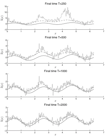
Fitted posterior means (i.e. solutions of (6) are given in Figure 1. This figure also gives the maximum likelihood solution
LTˆb= 1 2L
′
T
to which we refer as local time solution. Note that this is not quite the same as just the logarithm of the discretised local time since an interpolation to H2
h takes place.
Looking at Figure 1 it is clear that as the final time increases, the posterior mean converges to the true drift. Since the drift is smooth (C∞) convergence
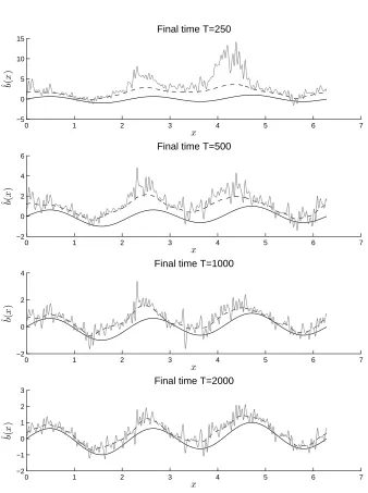
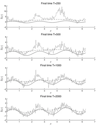
is unaffected by the specified prior. The prefactorηin the specification of the prior is critical - the quality of approximation of the true drift for medium range final times greatly depends on tuning this parameter as can be inferred contrasting Figures 2 and 3 to Figure 1.
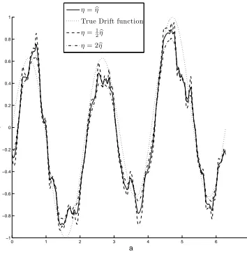
3.2. Optimal Smoothness Parameter. Further to Subsection 1.5, we use the expression (13) to derive optimal values for the parameterηand highlight potential problems with the empirical Bayes approach in this context.
Testing this for a single fixed sample path (T = 800), in the case k = 1, ǫ= 1, the resulting optimal values for η as a function of number of mesh elementsB are given in Figure 4 together with the behaviour of the normal-izing constant. The parameterǫhas been studied, too, optimizing over both parameters. The results are only slightly different, so in order to simplify the presentation, we restrict attention to the case of fixedǫ= 1.
0 1 2 3 4 5 6 7 −5
0 5 10 15
Final time T=250
x
ˆb(x
)
0 1 2 3 4 5 6 7
−2 0 2 4 6
Final time T=500
x
ˆb(x
)
0 1 2 3 4 5 6 7
−2 0 2 4
Final time T=1000
x
ˆb(x
)
0 1 2 3 4 5 6 7
−2 −1 0 1 2 3
Final time T=2000
x
ˆb(x
)
Fig 1. Posterior Means for increasing final timeT,η= 1
200
[image:12.595.154.489.137.575.2]0 1 2 3 4 5 6 7 −5
0 5 10 15
Final time T=250
x
ˆb(x
)
0 1 2 3 4 5 6 7
−2 0 2 4 6
Final time T=500
x
ˆb(x
)
0 1 2 3 4 5 6 7
−2 0 2 4
Final time T=1000
x
ˆb(x
)
0 1 2 3 4 5 6 7
−2 −1 0 1 2 3
Final time T=2000
x
ˆb(x
)
Fig 2. Posterior means for increasing final timeT,η= 1
2000
[image:13.595.153.491.122.575.2]0 1 2 3 4 5 6 7 −5
0 5 10 15
Final time T=250
x
ˆb(x
)
0 1 2 3 4 5 6 7
−2 0 2 4 6
Final time T=500
x
ˆb(x
)
0 1 2 3 4 5 6 7
−2 0 2 4
Final time T=1000
x
ˆb(x
)
0 1 2 3 4 5 6 7
−2 −1 0 1 2 3
Final time T=2000
x
ˆb(x
)
Fig 3. Posterior means for increasing final timeT,η= 1
2
[image:14.595.154.489.137.575.2]0 0.5 1 1.5 2 2.5 0
10 20 30 40 50 60 70 80 90 100
η
log Posterior normalisation constant
0 0.5 1 1.5 2 2.5
0.1 0.2 0.3 0.4 0.5 0.6 0.7 0.8 0.9
η
L2−distance of posterior mean from true b
B=50,bη=1.24
B=71,bη=1.28
B=100,ηb=1.24 B=141,ηb=1.1
B=50,ηb=1.5
B=71,ηb=1.6 B=100,bη=1.68
B=141,bη=1.74
Fig 4. Log-normalization constants andL2-distances vs. hyperparameterη
0 1 2 3 4 5 6 7
−1 −0.8 −0.6 −0.4 −0.2 0 0.2 0.4 0.6 0.8 1
a
b
η=ηb
True Drift function η=1
2ηb η= 2ηb
[image:15.595.212.393.121.376.2] [image:15.595.215.392.436.620.2]0
1
2
3
4
0 0.5 1 1.5 2 2.5
0 2 4 6 8 10 12 14
ε η
P(
η
,
ε
)
Fig 6. Log-normalization constant vs.ηandǫ– short path: T = 50
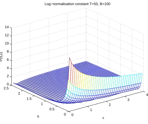
For shorter final times e.g. in the caseT = 50, especially when the local time is zero on some interval in the circle, the procedure sometimes yields optimal hyperparameters ηb = 0,bǫ = 0, which is of course unacceptable since neither prior nor posterior measures exist in this case; see Figure 6. We have investigated the phenomenon numerically and it seems that it is a manifestation of a problem at the analytical level, i.e. it does not seem to be an artifact of discretisation. However, an analytical treatment of the problem seems difficult, and since it is not unusual for empirical Bayes to yield optimal values on the boundary of the parameter space, we do not investigate the problem further.
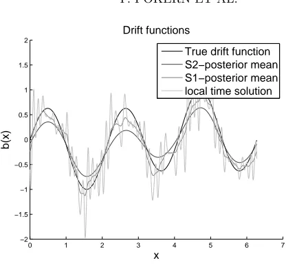
3.3. Order of Covariance Operator. Another aspect to study is the order of the covariance operator used in specifying the prior. Resulting posterior means for the force functions are given in figure 7 for the local time solution, the second-order covariance operator (i.e. (η∆ +I)−1) abbreviated to S1 and the fourth-order covariance operator (i.e. η∆2+I−1) abbreviated to S2. The parameters areT = 1000 andη= 1.
[image:16.595.160.449.117.360.2]0 1 2 3 4 5 6 7 −2
−1.5 −1 −0.5 0 0.5 1 1.5 2
x
b(x)
Drift functions
True drift function S2−posterior mean S1−posterior mean local time solution
Fig 7. Posterior means using S2, S1 priors and local time solution
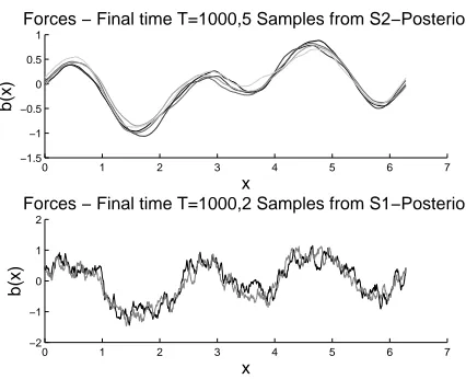
functions in the S1 and S2 cases in figure 8 for η = 101 but B = 500 finite elements to render the regularity of the sample paths more visible.
Gaussian Boundary Conditions. Further to the formal calculation pre-sented in Subsection 1.4, we implement a numerical solution of (12) using the same finite element implementation as above and implement the boundary conditions using the functional (9). For the sake of contiguous presentation, we consider the process
dx=−2 tanh(x−π)dt+dB, x(0) =π
(17)
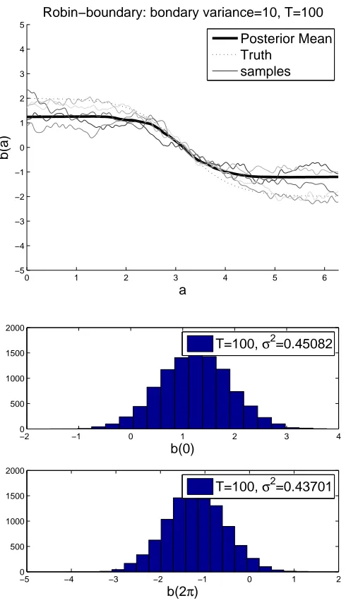
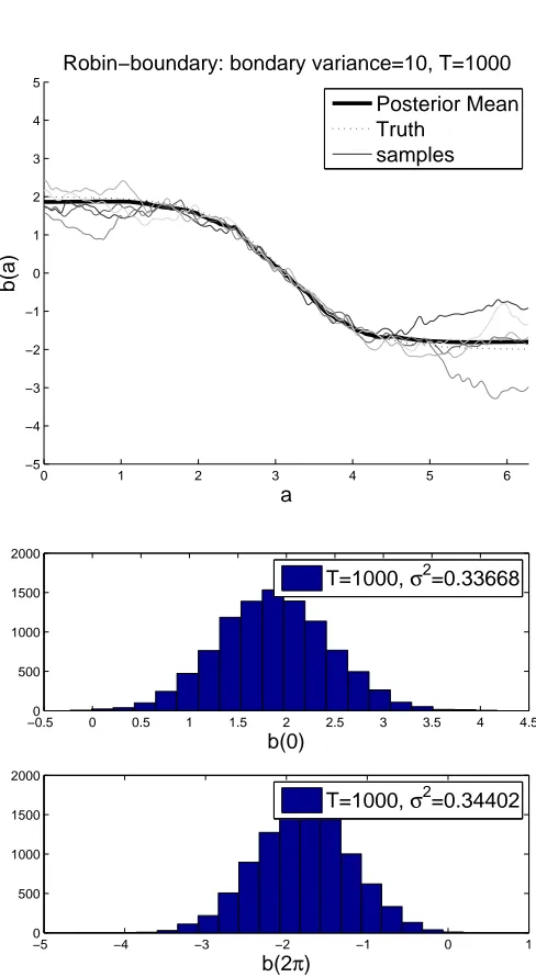
where the scaling factor 2 is chosen to make the process spend most of its time in [0,2π], so that it makes sense to choose y = 0 and z = 2π in Subsection 1.4. We use a smoothing constant η = 5 and a boundary point prior variance of σ2 = 10, as used in (12). Again, we use a sampler based on Exact Algorithm 1 from [1] with similarly small time increment δt as above. With these conventions, we obtain the plots in Figures 9, 10 and 11. Since our posterior measures on the space of force functions leave it unclear what happens to the process once it leaves [0,2π], we cannot decide whether ergodicity is maintained.
3.4. Rates of Posterior Contraction. Convergence is studied for the choice
[image:17.595.176.384.98.291.2]0 1 2 3 4 5 6 7 −1.5
−1 −0.5 0 0.5
x
b(x)
0 1 2 3 4 5 6 7
−2 −1 0 1 2
Forces − Final time T=1000,2 Samples from S1−Posterior
x
b(x)
Fig 8. Draws from posterior drifts, S1 and S2 cases
this value ofη, the difference between the MLE (in its finite element imple-mentation) and the Bayesian posterior mean is nearly invisible in any of the plots given before.
In considering how the posterior distribution converges as T → ∞ it is clear that marginalization of some form will be needed to make the con-vergence of measures on the infinite dimensional space H1(0,2π) amenable to numerical investigation. Since we are interested in the behaviour of the proposed method under mesh refinement, merely considering the finite di-mensional finite element discretisation as the marginalization is unhelpful. While many more sweeping marginalizations are conceivable, we will con-centrate on three marginalizations of the posterior measureµ:
• Point evaluation: Considerτ(u) =u(0.38π)
• Integration:Integrate against a test function:τ(u) =R02πu(a) sin(a)da
• Norms: Appropriate Hilbert Space norms: τ(u) = kukL2 or τ(u) = kukHγ, γ ∈(0,1).
Note that point evaluation and integration are linear operations, so that the posterior is expected to be Gaussian, whereas taking norms will result in distributions more akin toχ2.
[image:18.595.197.410.115.288.2]0 1 2 3 4 5 6 −5
−4 −3 −2 −1 0 1 2 3 4 5
a
b(a)
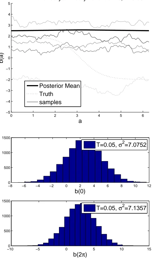
Robin−boundary: bondary variance=10, T=0.05
Posterior Mean Truth
samples
−8 −6 −4 −2 0 2 4 6 8 10 12
0 500 1000 1500
b(0)
T=0.05, σ2
=7.0752
−100 −5 0 5 10 15
500 1000 1500
b(2π)
T=0.05, σ2=7.1357
[image:19.595.182.427.170.584.2]0 1 2 3 4 5 6 −5
−4 −3 −2 −1 0 1 2 3 4 5
a
b(a)
Robin−boundary: bondary variance=10, T=100
Posterior Mean Truth
samples
−2 −1 0 1 2 3 4
0 500 1000 1500 2000
b(0)
T=100, σ2
=0.45082
−5 −4 −3 −2 −1 0 1 2
0 500 1000 1500 2000
b(2π)
T=100, σ2=0.43701
[image:20.595.181.426.158.585.2]0 1 2 3 4 5 6 −5
−4 −3 −2 −1 0 1 2 3 4 5
a
b(a)
Robin−boundary: bondary variance=10, T=1000
Posterior Mean Truth
samples
−0.50 0 0.5 1 1.5 2 2.5 3 3.5 4 4.5
500 1000 1500 2000
b(0)
T=1000, σ2
=0.33668
−5 −4 −3 −2 −1 0 1
0 500 1000 1500 2000
b(2π)
T=1000, σ2=0.34402
[image:21.595.180.424.138.583.2]4 6 8 10 12 14 16 18 −6
−4 −2 0 2
log2(Tf)
Error of Mean
Mean and Quartiles
4 6 8 10 12 14 16 18
−10 −8 −6 −4 −2 0 2
log2(Tf)
lo
g2
(V
a
ri
a
n
ce
) Sample Variance
LSQ fit, slope=−0.97532
Fig 12. Convergence of deviations of the posterior mean forb(0.42π)
the point value of ˆbhas a strong high-frequency component when subjected to Fourier transform. Looking at an eigenvalue analysis of the PDE (6) this would suggest that the final time needed to see the CLT-like decay of vari-ance like O(1/T) is very large and linked to the numerical resolution. In fact, one can perform a principal component analysis of the variance to find that most of the randomness resides in the high-frequency components of the right hand side of the discretised PDE.
To investigate this issue more closely, four different finite element resolu-tions,N ∈ {35,50,71,100} have been used to observe the decay of variances of the posterior marginalized means. Consulting the right hand side plot in Figure 13, where point evaluation b(0.42π) has been used to marginalize as before, it is apparent that a CLT-like decay of O(1/T) is only achieved for the lower resolutions. Furthermore, the 1/T-asymptotics take over at increasingly larger final times T with increasing number of mesh elements
N.
3.4.2. Integration against Test Function. On the other hand, when the procedure to marginalize the posterior means is to numerically integrate against the function sin(x), i.e. to consider the random variables
[image:22.595.183.428.126.324.2]independent of the chosen numerical resolution,N.
In conclusion, a CLT-like decay of variance is observed numerically for the posterior means as expected when evaluation is against a smooth functional; and this asymptotic is found to be robust against numerical resolution. For point evaluation, however, absence of the CLT-like decay of variance for the continuous PDE where the spectrum of the differential operator ∆2 is not
bounded (as opposed to its discretisation where it always is bounded) is supported by the numerical observations.
It would be interesting to investigate whether the intermediate slopes for the decay of variance observed in Figure 13 – e.g. for N = 100 the slope of approximately −0.4 – can be accounted for using the above-mentioned Fourier picture. While this is not central to the newly proposed Bayesian nonparametric estimation procedure, it might have mathematical merit.
3.4.3. Norms. Similar experiments can be performed when norms are used to examine convergence, although the resulting distribution will of course not be Gaussian but rather more likeχ2. Some example distributions can be seen in Figure 14.
Again, one can consider the mean and variance of posterior errors which is carried out in Figure 15. Note that convergence of the means is only observed in the L2 case with convergence in the H1 case only occurring beyond log2(Tf) ≥ 12 which is the regime where the finite mesh size is overcome by large final time, so that no convergence would be expected there in the case of increased resolution.
4. Application Example: Molecular Dynamics. In this section we give a brief application of the proposed non-parametric drift estimator to a toy example from Molecular dynamics. We start by explaining the origin of the data, apply the fitting algorithm to it and then compare the results to previous fits found in the literature.
4 6 8 10 12 14 16 18 −14
−12 −10 −8 −6 −4 −2 0 2
Variance of Posterior Marginal Mean − Smooth Marginalization
log2(Tf)
lo
g2
(V
a
r)
B=35 B=50 B=71 B=100
LSQ fit to B=100, slope=−1.0114
4 6 8 10 12 14 16 18
−10 −8 −6 −4 −2 0 2
Variance of Posterior Marginal Mean − Point Marginalization
log2(Tf)
lo
g2
(V
a
r)
B=35 B=50 B=71 B=100
LSQ fit to B=50, slope=−0.9985 LSQ fit to B=100, slope=−0.4385
[image:24.595.144.506.142.592.2]0 0.5 1 1.5 2 2.5 3 3.5 4 0
5 10 15 20 25 30 35 40 45
kbb- btruek 2 2
D
en
si
ty
T=200 T=800 T=3200 T=12800 T=51200
Fig 14. Distribution ofL2-marginals for various final timesT
4 6 8 10 12 14 16 18
0 2 4 6 8
log2(Tf)
Mean
L2 deviation H1 deviation/100
4 6 8 10 12 14 16 18
−15 −10 −5 0 5 10 15
log2(Tf)
Variance
L2 norm
H1 norm
[image:25.595.170.433.112.355.2] [image:25.595.166.435.412.627.2]Fig 16. Sketch of Dihedral Angle
is simulated using a damped-driven Hamiltonian system:
¨
x+γx˙− ∇V(x) =
s
2γ β W .˙
(18)
This is a second order hypoelliptic diffusion process driven by standard Brownian motion W,γ > 0 is the friction coefficient and β > 0 plays the role of inverse temperature. Details of the force field and potential V used here can be found in [10] and an overview of the use of Langevin dynamics in Molecular Dynamics simulations can be found in [22].
From a chemical point of view interest is focused on the dihedral angle
ω, which is the angle between the two planes in R3 formed by atoms 1,2,3 and atoms 2,3,4 respectively; see the sketch in Figure 16. Conformational change is manifest in this angle, and the Cartesian coordinates themselves are of little direct chemical interest. Hence it is natural to try and describe the stochastic dynamics of the dihedral angle in a self-contained fashion.
One MD run is produced using a timestep of ∆t = 0.1fs (Throughout this section, we use the time unit femtosecond abbreviated to fs. Note that 1f s= 10−15s.) and a Verlet variant (see p.435 in [22]) covering a total time ofT = 4·10−9s (4 nanoseconds). A section of the path of the dihedral angle as a function of time can be seen on the left of Figure 17; the corresponding histogram for the whole of the path is depicted to the right of that figure.
It should be stressed that the Itˆo process governing the behaviour of the dihedral angle ω is not of the form (1), in particular, it will have a non-constant diffusivity and be hypoelliptic of second order, so its regularity will beC1.
4.1. Fitting. We aim to non-parametrically estimate the drift function
[image:26.595.237.374.116.207.2]0 1 2 3 4 5
x 105
−3 −2 −1 0 1 2 3
t/fs
ω
(t)
Butane Samplepath − Langevin Dynamics
−40 −2 0 2 4
5 10
15x 10
4
ω
Histogram of Dihedral Angle
N=4⋅ 106
Fig 17. MD Samplepath Butane.
Left: First 500ps of sample path, Right: Histogram of whole sample path
variation
hXi= nX−1
i=0
(Xi+1−Xi)2 (19)
corresponds to hXi = T so that we have apparent diffusivity 1. To under-stand the next preprocessing step of subsampling, consider Figure 18 where we have plotted the apparent quadratic variation as a function of subsam-pling factork, i.e. we computed (19) using only everykth step of the Butane data. From this Figure, it is clear that the region k ∈ {1, . . . ,100} is not usable since this shows a step√k-law increase of apparent diffusivity – this mirrors the fact that the path actually has quadratic variation zero since it is of smoothness C1. The region k∈ {100, . . . ,500} also is not very usable since the apparent diffusivity varies strongly, so that the process is not ade-quately described by (1) on this timescale, either. On the timescale obtained for subsampling factors k∈ {1000, . . . ,5000} the apparent diffusivity varies little so that we settle for a subsampling factork= 1000 taking the observed apparent diffusivities form Figure 18 as indication that the dihedral angle process behaves qualitatively like a first order diffusion on those timescales. The attributed final time to make the diffusivity one isT = 1127.
[image:27.595.168.445.112.308.2]0 500 1000 1500 2000 2500 3000 3500 4000 4500 5000 0
500 1000 1500 2000 2500 3000 3500 4000
Subsampling rate
Diffusivity
σ
2
Fig 18. Apparent Diffusivity versus subsampling factor k
η = 0.02 we perform non-parametric estimation of the drift function in (1) for the Butane data set described above. The resulting posterior mean is given in Figure 19 where the solid line indicates the posterior mean and the shaded regions display one standard deviation credibility bands derived from the posterior measure. In the case of this dataset, the posterior normalization constant used in Subsection 3.2 yields an optimal hyperparameter ηb = 0, see Figure 20.
5. Existence and support of the prior measure.
5.0.1. Existence. We show in Appendix 10.1 that the covariance operator (∆2+I)−1 for the Gaussian measure
µ0=N
0,(∆2+I)−1 (20)
on L2(0,2π) exists, and that it is symmetric, non-negative and trace-class and can thus use Theorem 2.3.1 from [6] to establish the existence of a corresponding Gaussian measure.
5.0.2. Support. The Cameron-Martin-space for the measure µ0 is H =
Hper2 (0,2π) equipped with the norm kfk2H=k∆fk2L2+kfk2L2. So, we use a series representation of the random variableX∼µ0 as follows:
X =
∞ X
k=−∞
[image:28.595.206.396.114.270.2]0 1 2 3 4 5 6 7 −8
−6 −4 −2 0 2 4 6 8 10
a
b
(a
)
Butane data: Posterior Drift Functions
Fig 19. Posterior mean drift function for Butane data
0 0.2
0.4 0.6
0.8
0 0.2 0.4 0.6 0.8 1 1600 1800 2000 2200 2400 2600 2800 3000
ε
Butane−data, posterior log normalization constant
η
[image:29.595.189.417.123.330.2] [image:29.595.192.424.430.607.2]ek(x) =
1 √
π(k4+1)cos(kx) k >0
1
√
2π k= 0
1 √
π(k4+1)sin(kx) k <0
,
(22)
and theξk are iid. standard normal random variables. Theorem 3.5.1 in [6] guarantees that the representation (21) converges almost everywhere with respect to µ0. To find out whether X ∈ H
3 2−ǫ
per for 0< ǫ < 32, compute the appropriate seminorm as follows:
|X|2
H32−ǫ =
∞ X
k=−∞
ξk2|k|3−2ǫkekk2L2
=
∞ X
k=−∞
ξk2|k|3−2ǫ 1
1 +k4 ≤
∞ X
k=−∞
ξk2|k|−1−2ǫ.
The latter sum converges almost surely for any 32 > ǫ >0. Therefore, a draw from µ0 will almost surely be contained in H
3
2−ǫ for any ǫ > 0. Thus, we have found a Hilbert support of µ0.
6. Analysis of the PDE for the Posterior Mean. In this section we present a brief analysis of the PDE for the posterior mean, (6), establishing coercivity, continuity, symmetry and positivity of the differential operator under mild conditions on the local timeLT, and consequently existence and uniqueness of solutions.
Stability against small, admissible perturbation ofLT is also established and enables error estimates for the whole approximation process starting from the L2-error in the local time LT up to the numericalsolution u.
6.1. Analytical Setup. We write the PDE (6) with the choice A = ∆2 for the prior as
∆2+I+LT
u= 1
2L
′
T +W + ˜χ(·;X0, XT), u∈H2per([0,2π]) (23)
Here the PDE is solved in the weak H2-sense, i.e. we understand (23) to mean that we seek au∈H2
per([0,2π]) such that
Z 2π
0 ∆v(a)∆u(a) + (1 +LT(a))u(a)v(a)da=
Z 2π
0 −
1 2v
′(a)L(a) + (W + ˜χ(a;X
0, XT))v(a)da ∀v∈Hper2 . See [11] for details. We make use of the abbreviationf introduced in (1.3).
6.2. Coercivity. In order to move to a rigorous weak formulation of the PDE problem (23) we write it using the quadratic form
(25) aG(u, v) =
Z 2π
0
∆u(a)∆v(a) +u(a)G(a)v(a)da, u, v ∈Hper2 ([0,2π]) Assuming that the functionGis continuous, periodic, non-negative and not identically zero we obtain coercivity of this bi linear form:
Lemma 1. If function G is continuous, periodic, non-negative and not identically zero on[0,2π], then the formaG, defined in (25), is a continuous,
coercive, symmetric bi linear form, i.e. there are constantsα, C ∈R+ which may depend on G but not on u, v such that the following relations hold:
αkuk2H2 ≤aG(u, u) ∀u∈Hper2 ([0,2π]) (26)
aG(u, v)≤CkukH2kvkH2 ∀u, v∈Hper2 ([0,2π]) (27)
aG(u, v) =aG(v, u) ∀u, v∈Hper2 ([0,2π]) (28)
The proof of this lemma, in particular the proof of coercivity is slightly technical due to the differential operator involved being of fourth order, so that we present the proof of this lemma in Appendix 10.2.
Note that the local time LT almost surely satisfies the hypotheses on the function G needed in Lemma 1, a fortiori, LT + 1 also satisfies these hypotheses. For future use, we note down the quadratic form as used in in this case, i.e. forG=I+LT:
(29)
a(u, v) =
Z 2π
0
(30) ∆2u+ (I+LT)u= 1 2L
′
T +W + ˜χ(·;X0, XT)
has a unique solution u∈H2
per([0,2π]).
Proof. To show this, note that f from (1.3) is at least of regularity
H−1 since L
T ∈ Cper([0,2π]) ⊂ L2([0,2π]) and so its derivative will be in
H−1:L′
T ∈H−1([0,2π]), a fortioriwe haveL′T ∈H−2([0,2π]). Furthermore ˜
χ(˙;X0, XT) ∈ L2([0,2π]) and of course the same holds for the constant functionW, so the same argument yieldsf ∈H−2([0,2π]). We have shown in the above lemma 1 that the bi linear form associated with the partial differential operator ∆2 +I +LT is symmetric, continuous and coercive and hence defines an inner product onH2
per([0,2π]). Therefore, by the Riesz representation theorem, there exists a uniqueu∈Hper2 ([0,2π]) such that
Z 2π
0
∆u∆v+u(1 +LT)vdx=
Z 2π
0
vf dx ∀v∈Hper2 ([0,2π]).
Thisuis the unique weak solution to the PDE (30) in the statement of the theorem.
6.4. Continuous Dependence on LT. In this subsection we show robust-ness of the posterior mean against small errors in the local time LT that satisfy some positivity assumptions, in particular that the perturbed LT stays positive enough in a sense to be made precise. This result is not en-tirely obvious since the map from the local time LT to the posterior mean
u isnonlinear.
We establish the result by analyzing the PDE (23) for the perturbed local time ˜L:
∆2+I+ ˜Lu˜= 1 2L˜
′+ ˜χ(a, X
0, XT) +W, u˜∈Hper2 ([0,2π]) (31)
This PDE can be rewritten in terms of the unperturbed local time LT and the perturbation ˜L−LT:
∆2+I +Lu+∆2+I+L(˜u−u) + ( ˜L−L)˜u= 1 2L˜
′+ ˜χ(·;X
0, XT) +W Using that u satisfied the PDE (23), we can subtract this PDE from the previous one to obtain:
∆2+I+ ˜L(˜u−u) = 1 2
˜
L′−L′−u˜L˜−L
Note that we have assumed for the moment that W and ˜χ(·;X0, XT) are unperturbed which certainly for discrete time observations of initial and final condition is safe for ˜χ.
Suitable assumptions on ˜L are as follows: • L˜ ∈L∞([0,2π]), kL˜k<2kLTk∞ • L˜ ≥0
• R02πL˜(x)dx > 12T
The set of functions satisfying these conditions will be denoted by Λ and called admissible local times.
Lemma 2. For admissible perturbed local times L˜ ∈Λ, the perturbed bi linear form
˜
a(u, v) =
Z 2π
0
u∆2+I+ ˜Lvdx
(33)
is still coercive, symmetric and continuous on Hper2 ([0,2π]). The coercivity and continuity constants in Lemma 1 can be chosen such thatα and C are the same as those for the bi linear form (29) uniformly for allL∈Λ.
The proof of Lemma 1 was performed with robustness of constants to allow for this result.
The rest of the calculation then follows standard procedure:
αku˜−uk2H2 ≤˜a(˜u−u,u˜−u)
Now using the PDE for the perturbations, (32), to replace the right hand side, we obtain:
αku˜−uk2H2 ≤
Z 2π
0 1
2(˜u−u)( ˜L
′−L′
T)−(˜u−u)( ˜L−LT)˜udx =
Z 2π
0 −
1
2(˜u−u)
′( ˜L−L
T)−(˜u−u)( ˜L−LT)˜udx ≤ 12ku˜−ukH1 · kL˜−LTkL2(1 +ku˜k∞) ≤ 1
2ku˜−ukH2 · kL˜−LTkL2(1 +ku˜k∞) Dividing both sides byku˜−uk2
H2 we obtain that this norm is either zero or at least admits the following bound:
αku˜kH2 ≤ k 1
2L˜+ ˜χ(·;X0, XT) +WkL2 (35)
Due to a Sobolev embedding we have thatku˜k∞≤Cku˜kH2 for some suitable constant C > 0 so that we can use (35) to bound the term in brackets in (34). Additionally, use the fact that since ˜L∈Λ we have kL˜k∞ ≤2kLTk∞
to obtain the bound in the following theorem:
Theorem 3. There exists a constant C(W,kLk∞) > 0 such that for all admissible perturbed local times L˜ ∈ Λ the deviation of the perturbed posterior mean u˜ from the unperturbed posterior mean u is bounded in the
H2-norm:
∃C >0∀L˜ ∈Λ : ku˜−ukH2 ≤C(W,kLk∞)kL˜−LkL2 (36)
6.5. Summary of the Analysis. To summarize, it has been shown that the PDE for the posterior mean, (23) has a unique solution. Also, an H2 -bound for perturbations of this solution wrt. changes of the local time has been found. This enables stable numerical treatment which will be detailed in the sequel.
7. Existence and absolute continuity of the posterior. We em-ploy the Hajek-Feldman theorem (in the version given in [13], Theorem 2.23) to establish absolute continuity. To simplify the presentation, we use the prior measureµ0 is as given in (20). The covariance operator is
Q1 = (∆2+I)−1
and the posterior measure is Gaussian with covariance
Q2= (∆2+I+LT)−1
and meanu = ∆2+I+LT−1(12L′T +W + ˜χ(·;X0, XT)) where Section 6 showed that u∈H2
per([0,2π]).
Theorem4. The measuresµ0=N(0, Q1)andµ=N(u, Q2)onL2(0,2π)
are absolutely continuous with respect to each other.
Conjecture 1. The operatorQ
1 2
1Q
−12
Result1. Their Radon-Nikodym derivative is given by
dµ dµ0 ∝
exp 1 2 Z 2π 0
(LT(a) + 1)b2(a)−(L′T(a) + ˜χ(a;X0, XT) +W)b(a)da
(37)
The theorem 4 will be proved in three steps as an application of gen-eral theorems on Gaussian measures on Hilbert spaces. A proof of result 1 assuming that the conjecture 1 is true will be given after that.
We proceed in three steps showing firstly that the images of the square roots of the covariance operators, H0 =ImQ
1 2
1 and ImQ
1 2
2 agree. Secondly, we note that the difference of the respective means is an element of this image. Thirdly, we show that (Q−
1 2
1 Q
1 2
2)(Q
−12
1 Q
1 2
2)∗ −Id is Hilbert-Schmidt on L2.
Identity of Images. Note first that we can get to the image of Q
1 2
1 by characterizing it as follows:
ImQ 1 2 1 = Q 1 2
1f|f ∈L2
=
g|Q−
1 2
1 g∈L2
= g| Q− 1 2 1 g L2 <∞
But this norm is defined via an inner product, so that we get access toQ−11
by taking adjoints and noting that due to periodicity, boundary terms can be neglected. It is now possible to prove the claim as follows:
Q− 1 2 1 g L2 <∞ ⇔ Z 2π
0 g(∆
2+I)gdx <∞
We now use a H¨older estimate exploiting continuity of LT on the compact interval [0,2π] so that we continue the string of equivalent statements as follows:
⇔
Z 2π
0
g∆2+I+Lgdx <∞
Means are in the Range. We showed in Theorem 2 that the solution to the PDE for the posterior mean,u, is in H2
per([0,2π]). We found in the preceding step of the proof that this space is contained in the image ofQ
1 2
1 so that the difference of the means (which is justu) is as required.
Projector is only Hilbert-Schmidt different. We endeavour to show that the operator
(Q−
1 2
1 Q
1 2
2)(Q
−12
1 Q
1 2
2)∗−Id (38)
is Hilbert-Schmidt onL2. By definition, this is equivalent to showing that
S =
∞ X
n=1
(fn,(Q−
1 2
1 Q
1 2
2)(Q
−1 2
1 Q
1 2
2)∗fn)L2−(fn,Idfn)L2<∞ (39)
holds for some Hilbert basis{fn}∞n=1 of L2(0,2π).
We consider the basis {en}∞n=∞ given in (22). Note that these functions
are smooth. Setting yn =Q−
1 2
1 en, using the eigenvalue definition of square root of an operator it is straightforward to calculate yn =
√
1 +n4en. We can then reformulate (39) as follows:
S=
∞ X
n=−∞
(Q−
1 2
1 en, Q2Q−
1 2
1 en)L2−(en, en)L2 =X
n
(yn, Q2yn)L2 −(Q 1 2
1yn, Q
1 2
1yn)L2 =X
n
(yn,(Q1−Q2)yn)L2
Since Q2 = ∆2+I+LT−1 is the left hand side operator in the PDE for the posterior mean, (30), we know its inverse - the differential operator ∆2+I+LT; note that the domain is unimportant since we are dealing with smooth functionsen and yn throughout.
Q−21yn=
∆2+I +LT
yn= (n4+ 1)yn+LTyn ⇒yn= (n4+ 1)Q2yn+Q2(LTyn)
⇒Q2yn=Q1yn− 1
where we have exploited the fact that the basis (22) is an eigenbasis of Q1 with eigenvalues Q1yn= n4+11 yn in the last line.
So that the sumS can be continued as follows:
S =X
n
n4hyn, 1
n4+ 1Q2(LTyn)i =X
n 1
n4+ 1hQ2yn, LTyni
Here, symmetry of Q2 has been exploited. Next, we use the relation (40) again to substitute forQ2yn and we obtain:
S≤X
n
1
n4+ 1|(Q1yn, LTyn)L2|+ 1
n4+ 1|(Q2(LTyn), LTyn)L2|
≤X n
1
n4+ 1 1
1 +n4kynk 2
L2kLTk∞+kLTk2∞kQ2kk
ynk2L2
n4+ 1
! ,
where we have used thatQ2 is a bounded operator and again we have used H¨older’s inequality to eliminate LT. Now note that kynk2L2 = 1 +n4 which is straightforward to verify remembering that en are eigenfunctions of Q1. Overall we obtain
S ≤
∞ X
n=−∞
1
n4+ 1
kLTk∞+kLTk2∞kQ2k
<∞
It turns out that the sum S converges as long as the perturbation that turnsQ1 intoQ2 is an inverse differential operator of lower order than Q1 – if its order is only lower by one, summability of the sequence is not obtained and one has to exploit that only finite Hilbert-Schmidt norm is required (rather than the trace class property we showed here).
To summarize, all three hypotheses of the Hajek-Feldman theorem from [13] have been shown to hold so that absolute continuity of the posterior measure with respect to the prior measure has been shown.
centred Gaussian random variable with the desired covariance operator. In a second step we translate this random variable to obtain the desired mean. Throughout these two steps we keep track of the prefactors introduced and finally identify the product of those prefactors as the desired likelihood up to constants of integration.
7.1.1. Covariance: Multiplication by I +K. We multiply the random variable
X∼µ0
which is distributed according to the prior measure by the operator T =
Q
1 2
1Q
−1 2
2 . We intend to use theorem 6.4.5. from [6] which requires that the operatorK =T−I be Hilbert-Schmidt onH(µ0) =Hper2 . This requirement is more stringent than the fact established above that CC∗−I is
Hilbert-Schmidt. We do not show this fact, but state it as conjecture 1. Now forS=T−1, theorem 6.4.5. from [6] guarantees that
dµ0◦S−1
dµ0 ∝
exp
δK(b)−1 2|K(b)|
2 H2per
,
hold:
δKs(b)− 1 2|Kb|
2
H = trace(Ks)−(b, Ksb)− 1
2(Kb, Kb) =C+1
2(b, b)− 1
2(b, b)−(b, Ksb)− 1
2(Kb, Kb) =C+1
2(b, b)− 1
2((I+K)b,(I+K)b) =C+1
2
Z 2π
0
(∆b(a))2+b2(a)da
− 1 2
Z 2π
0
q
(∆2+I)−1p∆2+I+LTb
′′2
+q(∆2+I)−1p∆2+I+LTb
2
da
=C+1 2
Z 2π
0 (∆b(a))
2+b2(a)da
− 1 2
Z 2π
0
p
∆2+I+L Tb
· q(∆2+I)−1 ∂4
∂a4 +I
! q
(∆2+I)−1
! p
∆2+L Tbda
=C+1 2
Z 2π
0 (∆b(a))
2+b2(a)da−1 2
Z 2π
0
(∆b)2b2(a) +LTb2
da
=C−1
2
Z 2π
0
LT(a)b(a)2da,
where any unlabelled inner products refer toHand we have used a constant
C∈R. Considering only the start and end of these calculations we can now extend them to all ofL2by continuity considering the measurable extensions
c
Kwhere needed. We thus find that the random variableT X has a Gaussian distribution and is absolutely continuous with respect to X with Radon Nikodym derivative
dL(T X)
dL(X) ∝exp
−1 2
Z 2π
0
LT(a)b(a)2da
.
(41)
SinceT is a closed operator it is easy to see that the expected value ofT X
is still zero. The Covariance is obtained as follows:
Y =T X+h
whereh is given as the solution of the PDE (30), (∆2+I+LT)h=
1 2L
′
T + ˜χ(·;X0, XT) +W
Note that since the operator on the left hand side of this PDE is exactly the inverse of the covariance operator of the random variableT X, thish fulfils the requirement of lying inside the Cameron-Martin space of the measure L(T X) so that Corollary 2.4.3 from [6] yields absolute continuity of the translated measureL(Y) and gives the Radon-Nikodym derivative as
dL(Y)
dL(T X) = exp
Z 2π
0
h
(∆2+I+LT)h
i
(a)b(a)da− 1 2khk
2
H
(42)
We can neglect the second summand in the exponent since it does not depend onb (we can think of it as a normalizing constant). It is clear thatT X and
Y have the same covariance operators and that the expected value has been shifted so that EY =h.
7.1.3. Combining the Radon-Nikodym factors. Going from the random variable X to the random variable Y we have accumulated two Radon-Nikodym factors given by (41) and (42) respectively. Multiplying these two factors together we see that sinceL(X) =µ0
dL(Y)
dµ0 ∝
exp
1
2
Z 2π
0
LT(a)b(a)2−L′+ ˜χ(·;X0, XT) +W(a)b(a)
da
(43)
as desired for (4) to hold.
7.2. Rigorous Bayesian Framework. Writing down conditional probabil-ity measures like
P(b|{xt}Tt=0)
first define a product measure on the product space of path observations and drift functions and then multiply this measure by the desired likelihood to establish existence of a probability measure on the product space. It is then a straightforward matter to verify that the required marginal and con-ditional densities of that measure are as desired. For the sake of brevity, we shall not give details.
8. Estimating LT from discrete high-frequency observations. 8.1. General Remarks. In practice, the exact function LT is not avail-able, whereas what typically is available are observations of the diffusion pro-cess {Xti}Ni=1. We will consider the case of high-frequency observations, i.e. we assume constant final timeT, and thatN → ∞and maxi∈1,...,N1(ti+1−ti)→ 0. From the paper of Jacod [16] we can then getpointwise estimates of LT, i.e. he constructs random variablesU(h)n
T such that
P(|UTn(h)−λ(Hh)LT(0)|> ε)→0. (44)
Here,his some cutoff function, in the case of a histogram-like counting ap-proach this could be a step function centred at 0 with some fixed width δ
(corresponding to the bin width at that point). This estimator is formulated for the point value ofLT at 0 and there are uniformity statements asT is var-ied. Additionally, there are statements about the distribution obtained when the above difference between U and LT is scaled by √n, somewhat akin to asymptotic normality. However, there isnostatement about how estimates of LT at different points all obtained from the same time series behave, so obtaining statements for theL2-norm of the error is not straightforward.
8.2. post-factum local times. One way to approach this is to combine H¨older-Continuity of the local time with pointwiseL2-estimates as follows:
Let ˆLxi T =L
xi
T +ei be an estimate of the local time at the pointxi ∈[0,2π] with errorei. We extend this estimate simply to a constant function ˆL·T on the interval [xi, xi+1) and an estimate on the whole of [0,2π) is obtained by piecing these intervals together.
xi
|Lxi
T +ei−L x T|
2
dx≤
xi
ei2+ 2|ei||LTxi−LxT|+|L xi T −L
x T|2dx
≤2e2i|xi+1−xi|+ 2
Z xi+1
xi
|Lxi T −L
x T|2dx
≤2e2i|xi+1−xi|+ 2C
Z xi+1
xi
|xi−x|2αdx
= 2e2i|xi+1−xi|+ 2C
2α+ 1|xi+1−xi| 2α+1
where we have used that the local time L·
T is H¨older with exponent α and H¨older-constant C. To simplify, assume that an equispaced grid is used, i.e.
xi+1−xi= 2πM for someM ∈Nwhich may be large. Summing all the error contributions over the intervals i = 1, . . . , M we then obtain the following bound for theL2-error:
kLˆ·T −L·TkL2(0,2π)≤
M
X
i=1
2e2i|xi+1−xi|+ 2C
2α+ 1|xi+1−xi| 2α+1
≤4π max
i=1,...,Mei2 + 2C
2α+ 1 M
X
i=1
2π M
2α+1
= 4πmax i e
2 i +
22α+2π2α+1
2α+ 1 CM
−2α.
The trouble with this estimate is that M must be chosen large enough to compensate for C - but C is not known and depends on the continuous time sample path. Unless a-priori estimates of the H¨older constant of con-tinuity are available, this method can only be made to work ifM is chosen large enough as a function of the samplepath. Thus, overall convergence in probability can only be obtained if C can be bounded using only the high frequency data.
8.3. Admissible Perturbations. The restriction on admissible perturbed local times ˜L∈Λ is such that, in particular, local time functions LT2 taken at a later time T2 > T where T2−T is sufficiently small are admissible as perturbed local times ˜L. This is due to the joint continuity of local times,
9. Discussion. This paper is a first step towards Bayesian non-parametric drift estimation for Itˆo SDEs, providing a rigorously analyzed simple case as well as various numerical extensions of the proposed methodology.
Many of the limitations imposed are of a technical nature, so that several extensions seem likely possible:
• Treat Itˆo SDEs on the whole real line by considering appropriate func-tion spaces weighted with an invariant measure subject to ergodicity assumptions.
• Extend the methodology to higher dimensions. Dimensions two and three would be expected not to yield major complications, higher di-mensions make discretizing the PDE uncomfortable and very sparse grids would have to be used. Alternatively, methods to select base func-tions to arrive at a reduced spectral representation as used in quantum chemistry seem interesting.
• The use of the prior inverse covariance operatorA=η∆2+ǫIis largely illustrative, and it would be natural to consider other prior structures (Note that ∆ as used in Section 1.4 can be modified to impose a Markov property on prior and posterior which could be natural in some applications.) From a rigorous point of view, it should be noted that each such generalization leads to extra technical conditions to be checked.
Further work will consider genuinely discrete time observations (i.e. re-nounce the high frequency assumption). We will investigate the use of an MCMC data-augmentation scheme involving sampling alternatingly from local times given discrete time observations and drift functions.
In the discrete-time case, an interesting extension considers unknown (and possibly in-homogeneous) volatility for the observation process. There are natural methodologies for dealing with this problem which are developed in the Bayesian parametric literature (see for example [20]).
REFERENCES
[1] G.O. Roberts A. Beskos, O. Papaspiliopoulos. Retrospective exact simulation of diffusion sample paths with applications. Bernoulli, 12(6):1077–1098, 2006.
[2] R. A. Adams. Sobolev Spaces. Academic Press, 1975.
[3] Federico M. Bandi and Peter C. B. Phillips. Fully nonparametric estimation of scalar diffusion models. Econometrica, 71(1):241–283, 2003.
[6] V. I. Bogachev. Gaussian Measures. AMS, 1998.
[7] D. Braess. Finite Elemente, Schnelle L¨oser und Anwendungen in der Elas-tizit¨atstheorie. Springer, 1997.
[8] H. Br´ezis. Analyse fonctionelle – Th´eorie et applications. Dunod, 1999.
[9] Fabienne Comte, Valentine Genon-Catalot, and Yves Rozenholc. Penalized nonpara-metric mean square estimation of the coefficients of diffusion processes. Bernoulli, 13(2):514–543, 2007.
[10] B.R.Brooks et al. Charmm: A program for macromolecular energy, minmization and dynamics calculations. J. Comp. Chem., 4:187–217, 1983.
[11] L. C. Evans. Partial Differential Equations. AMS, 1998.
[12] A. W. van der Vaart F. H. van der Meulen and J. H. van Zanten. Convergence rates of posterior distributions for Brownian semimartingale models. Bernoulli, 12(5):863– 888, 2006.
[13] J. Zabczyk G. Da Prato. Stochastic Equations in Infinite Dimensions. CUP, 1992. [14] A. van der Vaart H. v. Zanten. Rates of contraction of posterior distributions based
on gaussian process priors. Annals of Statistics, 36:1435–1463, 2008.
[15] W. Hackbusch. Elliptic differential equations : theory and numerical treatment. Springer, 1992.
[16] J. Jacod. Rates of convergence to the local time of a diffusion. Annales de L’institut Henri Poincar´e, Probabilit´es et statistique, 34:505–544, 1998.
[17] S. Chib O. Elerian and N. Shephard. Likelihood inference for discretely observed nonlinear diffusions. Econometrica, 69(4):959–993, 2001.
[18] N. G. Polson and G. O. Roberts. Bayes factors for discrete observations from diffusion processes. Biometrika, 81(1):11–26, 1994.
[19] J.N. Reddy.An Introduction to the Finite Element Method. McGraw-Hill, 1984. [20] G. O. Roberts and O. Stramer. On inference for partially observed nonlinear diffusion
models using the metropolis-hastings algorithm. Biometrika, 88(3):603–621, 2001. [21] J. C. Robinson. Infinite-dimensional Dynamical Systems. CUP, 2001.
[22] T. Schlick.Molecular Modeling and Simulation, an Interdisciplinary Guide.Springer, New York, 2002.
[23] Y.A.Kutoyants.Statistical Inference for Ergodic Diffusion Processes. Springer, 2004.
10. Appendix A: Technical Proofs.
10.1. Existence of the Prior Measure. To show that the prior is well-defined in (20), we note that the operatorA= ∆2+I with domainD(A) =
Hper4 is positive definite and symmetric. Its inverse is compact since H4
can, in this case, be given explicitly as in (22). The associated eigenvalues areλk= k41+1. Furthermore, the operator A−1 is trace class since
∞ X
k=−∞ Z 2π
0 ek(a)(A
−1e
k)(a)da=
∞ X
k=−∞
1
k4+ 1 <∞.
Since the desired covariance operatorA−1 is thus symmetric, non-negative and trace-class, Theorem 2.3.1 from [6] guarantees the existence of a corre-sponding Gaussian measure.
10.2. Proof of Lemma 1. In this part we prove Lemma 1. Proof:
Linearity and symmetry of the bi linear form are clear from inspection of (25). In order to prove coercivity we proceed in stages. Firstly, the operator is split in two parts which will be dealt with in turn:
a(u, u) =
Z 2π
0 (∆u)
2+u2Gdx=a
1(u, u) +a2(u, u) where the two parts are given as
a1(u, u) =
Z 2π
0
(∆u)2dx a2(u, u) =
Z 2π
0
u2Gdx
First part of the Proof:a1. In this part of the proof, we use the Poincar´e inequality to get a lower bound on theH2- andH1-seminorm content of the quadratic form.
In order to be able to use the Poincar´e inequality, introduce the function
v(x) =u′(x)−u′(0)1(x).
Note thatv∈H01([0,2π]) sinceu′(0) =u′(1) due to periodicity (and having
chosen to consider a continuous version ofu′). Now consider the first integral
in the above inequality:
Z 2π
0 (∆u(x))
2dx≥Z 2π 0 (∆u)
2dx=Z 2π
0 (∆u−v
′+v′)2dx
=
Z 2π
0 (∆u−v
′)2+ 2(∆u−v′)v′+ (v′)2dx Now note that