doi:10.4236/ajcm.2011.11002 Published Online March 2011 (http://www.SciRP.org/journal/ajcm)
An O(k
2
+kh
2
+h
4
) Accurate Two-level Implicit Cubic Spline
Method for One Space Dimensional Quasi-linear Parabolic
Equations
Ranjan Kumar Mohanty1, Vijay Dahiya2
1Department of Mathematics, Faculty of Mathematical Sciences, University of Delhi, Delhi, India 2Department of Mathematics, Deenbandhu Chhotu Ram University of Science & Technology, Murthal, India
E-mail: [email protected], vijay_15dahiya@yahoo.com Received February 23, 2011; revised March 6, 2011; accepted March 6, 2011
Abstract
In this piece of work, using three spatial grid points, we discuss a new two-level implicit cubic spline method of O(k2 + kh2 + h4) for the solution of quasi-linear parabolic equation
, , , ,
xx x t
u f x t u u u , 0< x <1, t > 0 subject to appropriate initial and Dirichlet boundary conditions, where h > 0, k > 0 are grid sizes in space and time-directions, respectively. The cubic spline approximation produces at each time level a spline function which may be used to obtain the solution at any point in the range of the space variable. The proposed cubic spline method is applicable to parabolic equations having singularity. The stability analysis for diffusion- convection equation shows the unconditionally stable character of the cubic spline method. The numerical tests are performed and comparative results are provided to illustrate the usefulness of the proposed method.
Keywords: Quasi-Linear Parabolic Equation, Implicit Method, Cubic Spline Approximation,
Diffusion-Convection Equation, Singular Equation, Burgers’ Equation, Reynolds Number
1. Introduction
The use of cubic splines for the numerical solution of linear two point boundary value problems has been dis-cussed by Bickley [1], Fyfe [2], Albasiny and Hoskins [3] and Rubin and Khosla [4]. Later, Chawla et al [5,6] have developed fourth order accurate cubic spline methods for singular two point boundary value problems. In 1983, Jain and Aziz [7] have derived fourth order cubic spline method for the solution of general two point non-linear boundary value problems. Khan and Aziz [8] have used parametric cubic spline approach for the solution of a system of second order boundary value problems. Re-cently, Monoj Kumar et al [9-11], and Rashidinia et al [12-13] have discussed higher order cubic spline finite difference method for singular two point boundary value problems. A cubic spline technique for the solution of 1D heat equation was discussed by Papamichael and Whiteman [14]. This technique was extended by Fleck Jr [15] and Raggett and Wilson [16] for solving one-di- mensional wave equation. Archer [17] has developed a fourth order collocation method for quasi-linear parabolic equation. Jain and Lohar [18] have solved non-linear
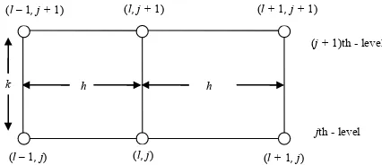
h h
k
(l, j) (l + 1, j) (l, j + 1)
(l – 1, j)
(l –1, j + 1) (l + 1, j + 1)
jth - level (j + 1)th - level
Figure 1. (Schematic representation of two-level scheme).
singular coefficients. The solution usually deteriorates in the vicinity of the singularity. In this paper, we refine our technique in such a way that the solution retains its order and accuracy everywhere in the solution region. In Sec-tion 5, we compared the proposed cubic spline method with the corresponding finite difference methods discussed in [20-22]. Finally, concluding remarks are given in Sec-tion 6.
2. The Two Level Implicit Cubic Spline
Method
Consider the quasi-linear parabolic equation in which the function u(x,t) satisfies
2
2 , , , ,x t , ,
u f x t u u u x t x
(1)
where the solution space is defined by
x t, 0 x 1,t 0
.
The initial condition is given by
,0 0
, 0 1u x u x x (2) and the boundary conditions are given by
0, 0
,
1, 1
, 0u t a t u t a t t (3) where u x a t0
, 0
and a t1
are given smooth func-tions.The region is covered in the usual manner by a rectangular net
x tl, j
lh jk,
, 0 l N1,j0 , where (N + 1)h = 1, and h > 0 and k > 0 are grid sizes in x- and t-directions, respectively. The mesh ratio parame-ter is given by
k h2
0. Let jl
U be the exact solution value of u(x,t) and j
l
u denotes a discrete ap-proximation to u(x,t) at the grid point
x tl, j
.We let S xj
denote the cubic spline interpolating the value jl
u at the jth time level, and is given by
3 3
1 1
2 2
1
1 1
1
6 6
,
6 6
, 1 1 1, 0
l j l j
j l l
j j l j j l
l l l l
l l
x x x x
S x M M
h h
x x x x
h h
u M u M
h h
x x x l N j
(4)
which satisfies at jth-level the following properties: 1) S xj
coincides with a polynomial of degree threeon each
xl1,xl
,l1 1
N1, j > 0, 2)
2
0,1 ,j
S x C and
3)
j, 0 1
1, 0j l l
S x u l N j ,
and where
j j
l xl
m U and
, , , ,
,j j j j j
l j l xx l l j l l tl
M S x U f x t U m U
0 1 1, 0
l N j .
We consider the following approximations:
j j
t t k (5)
1 1
j j j
l l l
U U U (6a)
1
1 1 1 1
j j j
l l l
U U U (6b)
1
j j j
t l l l
U U U k (7a)
1
1 1 1
j j j
t l l l
U U U k (7b)
1 1
2j j j j
l x l l l
m U U U h (8a)
1 1 3 1 4 1 2
j j j j j
l x l l l l
m U U U U h (8b)
, , , ,
j j j j
l l j l l t l
f f x t U m U (9a)
1 1, , 1, 1, 1
j j j j
l l j l l t l
f f x t U m U (9b)
1 1
1 1
ˆj j j j
l l l l
j j j
x l l l
m m ph M M
U ph f f
(10a)
1
1 1 1
1
1 ˆ
ˆ 2
6
2 6
j j
j j l l j j
l x l l l
j j
j j
l l
l l
U U h
m U M M
h
U U h
f f
h
(10b)
1
1 1 1
1
1 ˆ
ˆ 2
6
2 6
j j
j j l l j j
l x l l l
j j
j j
l l
l l
U U h
m U M M
h
U U h f f
h
(10c)
where
1 1
,
j j j j
l l l l
M f M f etc.
Further, we define
ˆj , , j,ˆj, j
l l j l l t l
f f x t U m U (11a)
1 1 1 1 1
ˆj , , j ,ˆj , j
l l j l l t l
f f x t U m U (11b) Then at each grid point
x tl, j
, the cubic spline method [image:2.595.64.277.78.170.2]R. K. MOHANTY ET AL. 13
21 2 1 12 ˆ 1 ˆ 1 10ˆ ˆ ,
1 1 , 0
j j j j j j j
l l l l l l l
h
U U U f f f T
l N j
(12)
where ˆj
2 2 4 6
l
T O k h kh h for 1 2
and 1
12 p . Note that, the initial and Dirichlet boundary conditions are given by (2) and (3), respectively. Incorporating the initial and boundary conditions, we can write the cubic spline method (12) in a tri-diagonal matrix form. If the differential Equation (1) is linear, we can solve the linear system using a tri-diagonal solver; in the non-linear case, we can use generalized Newton-Raphson method to solve the non-linear system (see Kelly [23], and Hage-man and Young [24]).
3. Derivation of the Cubic Spline Method
For the derivation of the cubic spline method (12) for the solution of the quasi-linear parabolic Equation (1), we simply follow the approaches given by Jain and Aziz [7].
At the grid point
x tl, j
, let us denote, , ,
,
a b
j j
ab a b l l
j j
l l
t
U f f
U t U x t f f m U (13)
Further at the grid point
x tl, j
, we may write thedif-ferential Equation (1) as
, , , ,
j j j j j
xx l l l j l l tl
U f f x t U m U (14a) Similarly,
1 1 1, , 1, 1, 1
j j j j j
xx l l l j l l t l
U f f x t U m U (14b) A difference method of accuracy of O h
4 for the dif-ferential Equation (1) in the absence of first derivative terms may be written as
2
6
1 2 1 12 1 1 10
j j j j j j
l l l l l l
h
U U U f f f O h (15) By the help of the notations (13) and simplifying (5)-(8b), we obtain
2 01j j
l l
U U kU O k (16a)
1 1 01
j j
l l
U U kU O kh (16b)
202
2
j j
t l t l k
U U U O k (17a)
1 1 2 02
j j
t l t l k
U U U O kh (17b)
2
2 4 11 6 30
j j
l l h
m m kU U O k h (18a)
2
3 1 1 11 3 30
j j
l l h
m m kU U O kh h (18b)
1 1
2 2 2
1 1 21
2 2
j j j
l l l
j j j
l l l
U U U
U U U kh U O k h
(19)
With the help of the approximations (5), (16a)-(18b), from (9a) and (9b), we obtain
01 11 2 2 4 02 30 2 6j j j j j
l l l l l
j j
l l
f f k U U
kU h U O k h
(20a)
1 1 01 11 02
2
3 30
2 3
j j j j j j
l l l l l l
j l
k
f f k U U U
h U O kh h
(20b)
Using the approximations (18a), (18b), (20a), (20b) and simplifying (10a), we get
2
11 30
2 2 4
ˆ 1 12
6
j j
l l h
m m kU p U
O k kh h
(21)
From (21), it is easy to verify that for 1 12
p , we have
2 2 4
11 ˆj j
l l
m m kU O k kh h (22a) Similarly, from (10b) and (10c), we have
2 1 3
1 1 11
ˆj j
l l
m m kU O kh k h h
(22b)
Finally, by the help of the approximations (5), (16a)-(17b), (22a)-(22b), from (11a) and (11b), we get
01 11 02
2 2 4
ˆ
2
j j j j j j
l l l l l k l
f f k U U U
O k kh h
(23a)
1 1 01 11 02
2 1 3 ˆ
2
j j j j j j
l l l l l k l
f f k U U U
O kh k h h
(23b)
Now differentiating the differential Equation (1) with respect to ‘t’ at the grid point
x tl, j
, we obtain arela-tion of the form
02 01 11 21
j j j j
l l l l
U U U U
(24)
Using the approximations (19), (23a), (23b) and by the help of the relation (24), from (12) and (15), we obtain the local truncation error
2
2 2 4 6 02
ˆ 1 2
2
j j
l l
kh
T U O k h kh h (25) The proposed cubic spline method (12) to be of
2 2 2 4
O k h kh h , the coefficient of kh2 in (25) must be zero. Thus we obtain the value of 1 2, for which
2 2 4 6
ˆj l
4. Cubic Spline Scheme for Parabolic
Equation with Singular Coefficients
Consider the linear parabolic equation of the form
2
2 , ,
0 1, 0
u u D x u E x u g x t
t x x x t (26)
subject to appropriate initial and Dirichlet boundary con-ditions are prescribed by (2) and (3), respectively. As-sume that the functions D x
, E x
and g x t
,
2 C .For D x
1 ,x E x
1
x2 , the equation above represents linear parabolic equation with singular coeffi-cients. For 1,D x
x, E x
x2 , the above parabolic equation becomes a cylindrical and spheri-cal problem for 1 and 2, respectively.Applying the formula (12) to the differential Equation (26), we get
2
1 1 1 1 1 1 1
1 1 1 1 1 1 1
ˆ 2
12 ˆ ˆ
10 , 1 1 , 0,1, 2,
j j j j j j
l l l tl l l l l
j j j j j
l t l l l l l l
j j j j
tl l l l l l
h
u u u u D m E u
g u D m E u g
u D m E u g l N j
(27) where
,
, j
,
l l l l l l j
D D x E E x g g x t ,
1 , 1 , 1 ,
j
j
l l l l l l
D D x h E E x h g g x h t etc. At the grid point
x tl, j
, let us denote, ,
a b a b a b
ab a b ab a b ab a b
D E g
D E g
x t x t x t
(28)
Note that, the cubic spline sheme (27) is of
2 2 4
O k kh h accuracy for the approximate solution of Equation (26). However, the scheme (27) fails to compute at l = 1 when the coefficients D x
x,
2E x x etc. In order to get a meaningful cubic spline scheme of O k
2kh2h4
accuracy in com-pact operator form, we need the following approxima-tions:
2
3 1 00 10 2 20
l h
D D hD D O h (29a)
2
3 1 00 10 2 20
l h
E E hE E O h (29b)
2
3 1 00 10 2 20 j
l h
g g hg g O h (29c) where
00 10 2 20 3
00 10
2
, , ,
, , etc.
l
l l l
j j
l xl
D D D D
x x x
g g g g
Now, by the help of the approximations (5)-(10c) and (29a)-(29c), neglecting high order terms, we can re-write the scheme (27) as a two-level implicit cubic spline scheme in operator compact form
2 1
0 1 2
2
0 1 2
2
2 1 1 N, 0,1, 2,
j
x x x l
j
x x x l
R R R u
S S S u g
l j
(30) where
2 20 00 20 10 00 00 10
2
1 00 10 00 00
2
2 00 20 10 00 00
2
0 10 0
2
0 10 0
1 1
1 1
2 00 2
2 00 2
12 ,
24
, 2
12 2 ,
4
1 ,
12
1 ,
12
1 1 6 ,
12
1 1 6 ,
12 1 , 12 2 1 , 12 2 h
P E h E D E D E
h
P E D D D
h
P D h D E D E
h
R D P
h
S D P
R P
S P
h
R D P
h
S D P
g
2
00 20 10 00 00 10
12 ,
12k g h g D g D g
and
1 1
2 2
1 2
x lu ul ul
and
1 1
2 2
x lu ul ul
are averaging and central difference operators with re-spect to x-direction etc. The cubic spline scheme (30) has a local truncation error of O k
2kh2h4
and is free from the terms 1
l1
, and hence, it can be solved for l = 1(1)N in the region 0 < x < 1, t > 0.Now consider the linear singular parabolic equation
2
2 2 , , 0 1, 0
u u u
u g r t r t
r r t
r r
(31)
R. K. MOHANTY ET AL. 15
3 20 2 l 10,D r E
420 6 l
E r etc. in Equation (30), we can get a two level implicit cubic spline scheme of O k
2kh2h4
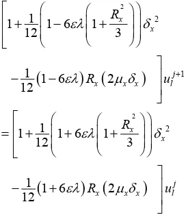
for the solution of linear singular parabolic Equation (31).Now, consider the linear diffusion-convection para-bolic equation
2
2 , 0 1, 0
u u u
x t
t x
x
(32)
The constant terms 0 and 0 are called the dif-fusivity and convective terms, respectively. For 0 , the problem is said to be convection dominated problem. Substituting
10 20 00 10 20 00 10 20
, 0
D D D E E E g g g
in the formula (30), we obtain a two-level implicit cubic spline scheme
2
2 2
1
2
1
1 1 6 1
12 3
1
1 6 2
12
1
1 1 6 1
12 3
1
1 6 2
12
x x
j
x x x l
x x
j
x x x l
R
R u
R
R u
(33)
where Rx h
2 represents the cell-Reynolds number. The scheme (33) is of O k
2h4
and consis-tent with the differential Equation (32). Further note that, the scheme (33) is identical with the scheme discussed by Jain et al [20]. It has been shown that, the scheme (33) is unconditionally stable and using this scheme computa-tional result for the solution of Equation (32) is reported in [20].5. Numerical Results
In order to demonstrate the application of the proposed cubic spline method, we have solved the following four
problems whose analytical solutions are known to us. The right-hand side homogeneous functions, initial and boundary conditions can be obtained using the exact so-lution as a test procedure. We have also compared the proposed cubic spline method with the corresponding finite difference method of O k
2kh2h4
discussed in [20-22]. We have solved the system of linear differ-ence equations using a tri-diagonal solver and the system of non-linear difference equations by Newton-Raphson method (see Kelly [23], and Hageman and Young [24]). All computations were performed using double length arithmetic.Example 1: (Linear parabolic equation with singular coefficients)
22 2
1 1
, , 0 1, 0
u u u
u g x t x t
x x t
x x
(34)
The exact solution is given by u(x,t) = exp(-εt) sinhx. The root mean square (RMS) errors at t = 1.0 are tabu-lated in Table 1 for 1.6 and small values of ε> 0.
Example 2: The Equation (31) is solved whose exact solution is u(r,t)=exp(-t) coshr. The RMS errors at t = 1.0 are tabulated in Table 2 for α = 1 and 2 for a fixed value of 1.6.
Example 3: (Burgers’ Equation ) 2
2 , 0 1, 0
u u u u x t
t x
x
(35)
The exact solution is given by
2 2 2 πsin(π ) exp π ,
2 cos(π ) exp π
x t
u x t
x t
, where
1 0
e R
is termed as a Reynolds number. The RMS errors at t = 1.0 are tabulated in Table 3 for different values of Re and
for a fixed value of 1.6.
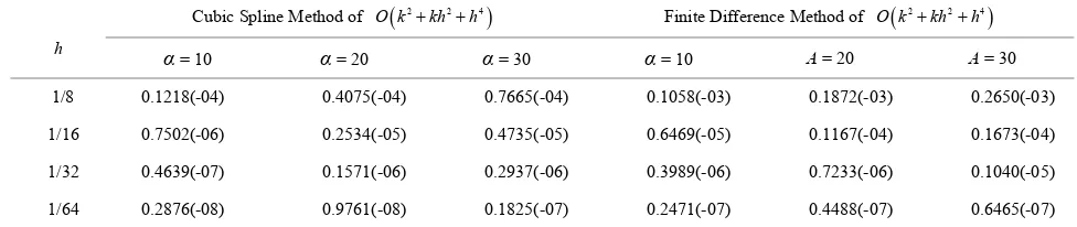
Example 4: (Non-linear Parabolic Equation )
2
2 , , 0 1, 0
u u u u g x t x t
t x
x
(36)
The exact solution is given by u(x,t)=exp(-t) sin(
x
). The RMS errors at t = 1.0 are tabulated in Table 4 for various values of α for a fixed parameter value of [image:5.595.98.234.290.447.2]1.6 .
Table 1. Example 1: The RMS errors.
h
Cubic Spline Method of O k
2kh2h4
Finite Difference Method of O k
2kh2h4
ε= 0.1 ε = 0.01 ε= 0.001 ε= 0.1 ε = 0.01 ε = 0.001
[image:5.595.55.540.637.723.2]Table 2. Example 2: The RMS errors.
h
Cubic Spline Method of O k
2kh2h4
Finite Difference Method of O k
2kh2h4
α = 1 α = 2 α = 1 α = 2
1/8 0.9604(-06) 0.1127(-05) 0.1054(-04) 0.1300(-04)
1/16 0.6378(-07) 0.7064(-07) 0.6997(-06) 0.8172(-06)
1/32 0.4107(-08) 0.4400(-08) 0.4511(-07) 0.5105(-07)
[image:6.595.55.541.234.336.2]1/64 0.2606(-09) 0.2740(-09) 0.2866(-08) 0.3187(-08)
Table 3. Example 3: The RMS errors.
h
Cubic Spline Method of O k
2kh2h4
Finite Difference Method of O k
2kh2h4
Re = 103 Re = 104 Re = 105 Re = 103 Re = 104 Re = 105
1/8 0.6442(-07) 0.6822(-09) 0.6887(-11) 0.1467(-06) 0.1612(-08) 0.1628(-10)
1/16 0.3278(-08) 0.4114(-10) 0.4274(-12) 0.8809(-08) 0.9820(-10) 0.9932(-12)
1/32 0.1244(-09) 0.1613(-11) 0.1688(-13) 0.5318(-09) 0.5925(-11) 0.5994(-13)
1/64 0.8884(-11) 0.9424(-13) 0.9870(-15) 0.3280(-10) 0.3494(-12) 0.3706(-14)
Table 4. Example 4: The RMS errors.
h
Cubic Spline Method of O k
2kh2h4
Finite Difference Method of O k
2kh2h4
α= 10 α= 20 α= 30 α= 10 Α= 20 Α= 30
1/8 0.1218(-04) 0.4075(-04) 0.7665(-04) 0.1058(-03) 0.1872(-03) 0.2650(-03)
1/16 0.7502(-06) 0.2534(-05) 0.4735(-05) 0.6469(-05) 0.1167(-04) 0.1673(-04)
1/32 0.4639(-07) 0.1571(-06) 0.2937(-06) 0.3989(-06) 0.7233(-06) 0.1040(-05)
1/64 0.2876(-08) 0.9761(-08) 0.1825(-07) 0.2471(-07) 0.4488(-07) 0.6465(-07)
6. Final Remarks
We presented a new cubic spline discretization strategy of O k
2kh2h4
for the solution of one-space di-mensional quasi-linear parabolic partial differential equa-tions. The proposed method with a little modification is applicable to singular parabolic problems. For singular problems, our numerical results show that the new cubic spline method may be advantageous compared with the corresponding finite difference method discussed in [20-22]. Numerical results for non-linear problems also show better as compared to the method discussed in [20-22], and numerical oscillation do not appear for high Reynolds number.7. Acknowledgement
The authors thank the reviewers for their valuable sug-gestions, which substantially improved the standard of
the paper.
8. References
[1] W. G. Bickley, “Piecewise Cubic Interpolation and Two Point Boundary Value Problems,” Computer Journal, Vol. 11, No. 2, 1968, pp. 206-208.
[2] D. J. Fyfe, “The Use of Cubic Splines in the Solution of Two Point Boundary Value Problems,” Computer Jour-nal, Vol. 12, No. 2, 1969, pp. 188-192.
doi:10.1093/comjnl/12.2.188
[3] E. L. Albasiny and W. D. Hoskins, “Increased Accuracy Cubic Spline Solutions to Two Point Boundary Value Problems,” Journal of the Institute of Mathematics and its
Applications, Vol. 9, No.1, 1972, pp. 47-55.
doi:10.1093/imamat/9.1.47
[4] S. G. Rubin and P. K. Khosla, “Higher Order Numerical Solutions Using Cubic Splines,” American Institute of Aeronautics and Astronautics Journal. Vol. 14, No.7, 1976, pp. 851-858.
[image:6.595.52.540.369.472.2]Me-R. K. MOHANTY ET AL. 17 thod for Singular Two Point Boundary Value Problems,”
International Journal of Computer Mathematics, Vol. 24, No. 3-4, 1988, pp. 291-310.
doi:10.1080/00207168808803650
[6] M. M. Chawla, R. Subramanian and H. L. Sathi, “A Fourth Order Spline Method for Singular Two Point Boundary Value Problems,” Journal of Computational and Applied Mathematics, Vol. 21, No. 2, 1988, pp. 189-202.doi:10.1016/0377-0427(88)90267-1
[7] M. K. Jain and T. Aziz, “Cubic Spline Solution of Two Point Boundary Value Problems with Significant First Derivatives,” Computer Methods in Applied Mechanics and Engineering,Vol. 39, No. 1, 1983, pp. 83-91.
doi:10.1016/0045-7825(83)90075-0
[8] A. Khan and T. Aziz, “Parametric Cubic Spline Approach to the Solution of a System of Second Order Boundary Value Problems,” Journal of Optimization Theory and
Applications, Vol. 118, No. 1, 2003, pp. 45-54.
doi:10.1023/A:1024783323624
[9] Manoj Kumar, “A Fourth Order Spline Finite Difference Method for Singular Two Point Boundary Value Prob-lems,” International Journal of Computer Mathematics, Vol. 80, No.12, 2003, pp. 1499-1504.
doi:10.1080/0020716031000148179
[10] Manoj Kumar, “Higher Order Method for Singular Boundary Value Problems by Using Spline Function,”
Applied Mathematics and Computations, Vol. 192, No.1, 2007, pp. 175-179.doi:10.1016/j.amc.2007.02.156
[11] Manoj Kumar and P. K. Srivastava, “Computational Techniques for Solving Differential Equations by Cubic, Quintic and Sextic Spline,” International Journal for Computational Methods in Engineering Science and Me-chanics, Vol. 10, No. 1, 2009, pp. 108-115.
doi:10.1080/15502280802623297
[12] J. Rashidinia, R. Mohammadi and M. Ghasemi, “Cubic Spline Solution of Singularly Perturbed Boundary Value Problems with Significant First Derivatives,” Applied Ma- thematics and Computations, Vol. 190, No. 2, 2007, pp. 1762-1766.
[13] J. Rashidinia, R. Mohammadi, R. Jalilian and M. Ghasemi, “Convergence of Cubic Spline Approach to the Solution of a System of Boundary Value Problems,” Applied Ma-thematics and Computations, Vol. 192, No. 2, 2007, pp. 319-331.doi:10.1016/j.amc.2007.03.008
[14] N. Papamichael and J. R. Whiteman, “A Cubic Spline Technique for the One-dimensional Heat Equation,” IMA Journal of Applied Mathematics, Vol. 11, No. 1, 1973, pp. 111-113.doi:10.1093/imamat/11.1.111
[15] J. A. Fleck Jr., “A Cubic Spline Method for Solving the Wave Equation of Non-linear Optics,” Journal of Com-putational Physics,Vol. 16, No. 4, 1974, pp. 324-341.
doi:10.1016/0021-9991(74)90043-6
[16] G. F. Raggett and P. D. Wilson, “A Fully Implicit Finite Difference Approximation to the One-dimensional Wave Equation Using a Cubic SplineTechnique,” Journal of the
Institute of Mathematics and its Applications, Vol. 14, No. 1, 1974, pp. 75-77.doi:10.1093/imamat/14.1.75
[17] D. Archer, “An O(h4) Cubic Spline Collocation Method
for Quasi-linear Parabolic Equation,” SIAM Journal of Numerical Analysis,Vol. 14, No. 4, 1977, pp. 620-637.
doi:10.1137/0714042
[18] P. C. Jain and B. L. Lohar, “Cubic Spline Technique for Coupled Non-linear Parabolic Equations,” Computers & Mathematics with Applications,Vol. 5, No. 3, 1979, pp. 179-195.doi:10.1016/0898-1221(79)90040-3
[19] J. Rashidinia and R. Mohammadi, “Non-polynomial Cu-bic Spline Methods for the Solution of Parabolic Equa-tions,” International Journal of Computer Mathematics, Vol. 85, No.5, 2008, pp. 843-850.
doi:10.1080/00207160701472436
[20] M. K. Jain, R. K. Jain and R. K. Mohanty, “A Fourth Order Difference Method for the One-dimensional Gen-eral Quasi-linear Parabolic Partial Differential Equation,”
Numerical Methods for Partial Differential Equations, Vol. 6, No.4, 1990, pp. 311-319.
doi:10.1002/num.1690060403
[21] R. K. Mohanty, “An O(k2 + h4) Finite Difference Method
for One Space Burgers’ Equation in Polar Coordinates,”
Numerical Methods for Partial Differential Equations, Vol. 12, No. 5, 1996, pp. 579-583.
doi:10.1002/(SICI)1098-2426(199609)12:5<579::AID-N UM3>3.0.CO;2-H
[22] R. K. Mohanty and M. K. Jain, “Single Cell Finite Dif-ference Approximations of O(kh2 + h4) for (u/n) for
one Space Dimensional Non-linear Parabolic Equations,”
Numerical Methods for Partial Differential Equations, Vol. 16, No.4, 2000, pp. 408-415.
doi:10.1002/1098-2426(200007)16:4<408::AID-NUM5> 3.0.CO;2-J
[23] C. T. Kelly, “Iterative Methods for Linear and Non-linear Equations,” SIAM Publication, Philadelphia, 1995. [24] L. A. Hageman and D. M. Young, “Applied Iterative