Design and Implementation a Real Time Targets Tracking Simulation in ADT Radar

Journal of Engineering and Applied Sciences 15 (2): 730-741, 2020 ISSN: 1816-949X

© Medwell Journals, 2020

Target trajectory

Angle Range

Target

Radar

Design and Implementation a Real Time Targets Tracking

Simulation in ADT Radar

1

_{Solaiman Al Jahoush,}

_{Abd Elrazzak Badawieh and}

_{Ali Kazem}

1, 2

_{Department of Electronic and Telecommunication Engineering,}

Damascus University, Damascus, Syria

3

_{Higher Institute for Applied Sciences and Technology, Damascus, Syria}

Abstract: The Automatic Detection and Track (ADT) radar is one of the most important types of modern radar. This radar rapidly scans a limited angular sector to maintain tracks with a moderate data rate, on more than one target within the coverage of the antenna. It is used for air-defense radars, aircraft landing radars and in some airborne intercept radars to hold multiple targets in track. The aim of this research is to study the tracking algorithm used in targets tracking such as tracking filters, tracking gate and data association. Firstly, we will study the basic principles of these algorithms by MATLAB tools, so we can study all advantages and disadvantages of these algorithms, after that we will design a software tools by visual C++ to implementation these algorithms in real time mode, so that, we can improve this algorithm and represent radar work very close to reality. Firstly, in this research, we will use the basic filters like (α-β), (α-β-γ) and Kalman filter then in the next experiments we can easily use this simulation to add newest filters and algorithms like Extended Kalman Filter (EKF), Particles Filter (PF), maneuver detector algorithm, Multi Model Interaction (MMI) etc. Key words: Tracking radar, Kalman filter, tracking filter, target tracking algorithms, airborne, software tools

INTRODUCTION

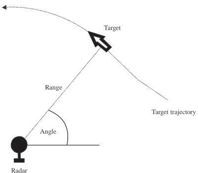
The basic tracking scenario consists of sensors which produce noisy measurements, for example, azimuth angle measurements as illustrated in Fig. 1. The purpose of tracking algorithm is to determine the target trajectory using the sensor measurements. There is additional prior which had poor or no MTI or any other means for reducing clutter. Its performance was a disaster when used with poor radars. A tracking system can be designed to recognize and eventually eliminate clutter echoes that information on the dynamics of targets which restricts the forms of target trajectories into those that are possible when the laws of physics are taken into account.

ADT requires a good radar that eliminates clutter echoes and other undesired signals. When ADT was first introduced it was mistakenly applied to the existing radars don’t form logical tracks but it takes time and computer capacity which might not be available when a large number of targets must be maintained in track. Thus, good tracking starts with good radar that eliminates unwanted clutter echoes and other extraneous signals. When clutter targets cannot be completely eliminated by Doppler processing, the ADT radar has to employ CFAR to maintain a constant false-alarm rate.

Function of ADT: The ADT consist of these stages: the track of a target in 2D can be determined from

Fig. 1: Radar generates angle and range measurements of the target and the purpose is to determine the target trajectory

surveillance radar Plan Position Indicator (PPI) display by plotting the target coordinates as they move when measured from scan to scan.

At its most simple this tracking function can be performed by a radar operator marking the face of the cathode ray tube with a pen. This is an inaccurate process

Corresponding Author: Solaiman Al Jahoush, Department of Electronic and Telecommunication Engineering,

J. Eng. Applied Sci., 15 (2): 730-741, 2020

1 2 3

4 5 6

50 45 40 35 30 25 20 15 10 5 0

T

a

rg

et

a

c

ce

le

ra

tio

n

m

/s

ec

2

0 20 40 60 80 100 120 140 160 180 Target angle

1-Rc = 1 nmi 2-Rc = 2 nmi 3- Rc = 3nmi 4- Rc = 4 nmi 5- Rc = 10 nmi 6- Rc = 50 nmi

1

2

3 4 5 6 Rmin = Rc

r (t) Vt

Vr V

X Y

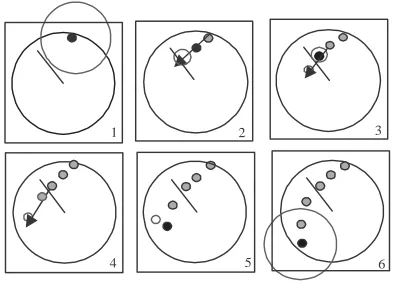
Fig. 2: ADT stages

and limits the number of targets that can be handled at one time. Automatic trackers operate as follows Fig. 2 (Hanscom Air For Base):

Target detection: Target is detected as the received echo exceeds a threshold. There is no information about its velocity. The software constrains the uncertainty to are as on able value for an aircraft target (large circle). Track initiation and association: Target is detected again displaced in range and angles but within the uncertainty boundary. A crude velocity estimate is made and the position where the target will appear next is predicted. The uncertainty is still large as the position and velocity estimates are not good, association is used when there is more than one radar return in the tracking gate or when we track more than one target.

Track update and smoothing: The target appears within this uncertainty boundary and recursive tracking filters estimates and improves both position and velocity and the next sample prediction is made with a smaller position uncertainty.

Track termination: The actual target position falls outside the position uncertainty boundary because it has accelerated and the prediction algorithm only used position and velocity. Track is lost a new target is detected with unknown velocity. In our research we will focus on two type of algorithms used in target tracking operation:

C Data association algorithm

C Tracking filters

MATERIALS AND METHODS

Technical point in target tracking: Before speaking about tracking algorithms, we will focus on some technical point must be conceder in target tracking.

Fig. 3: Pseudo-acceleration problems

Fig. 4: Pseudo-acceleration problems by MATLAB Selection of coordinates for tracking: For the two dimensional radar the natural coordinates for tracking are the slant Range R and azimuth θ coordinates. It is the one generally used. However, this coordinate system has an important disadvantage. Specifically when a target going in a straight line with a constant velocity flies by the radar at close range, a large geometry-induced acceleration is seen for the slant range even though the target itself has no acceleration. This acceleration is sometimes referred to as the pseudo acceleration of the target. It is illustrated in Fig. 3.

The closer the target flies by the radar, the larger is the maximum geometry-induced acceleration seen for the slant range coordinate. The maximum value for this acceleration is given by Eq. 1:

(1) 2

max c

v =

R



Where:

v : The target velocity

Rc : The closest approach range of the target to the radar

By studying this case using MATLAB Fig. 4:

(2)

J. Eng. Applied Sci., 15 (2): 730-741, 2020

Gate 1

Gate 2 d

d

X1 X2 Y

Y1 Y2

X

(3)

VrV cos

(4)

Vr (t) = Vr max cos (t)

(5) 2

2

V R min

a (t) = - sin (t) r (t)

r (t)  sin (t)

(6) 2

3

V

a (t) - sin (t) : R min Rc

R min

  

We note that a maximum value, obtained at the cross-range Rc, θ = π/2 so: we select x, y coordinate. If we are measuring the target Range R and azimuth angle θ but keep track of the target using the East-North x, y coordinates of the target then errors in the measurement of R and θ are not linearly related to the resulting error in x and y because the conversion equations are given by (Eq. 7 and 8):

(7)

x R cos

y R sin

 

 

where, θ is the target angle measured relative to the x axis. In this case how to simply handle this situation. Basically what is done is to linearize last tow equations by using the first terms of a Taylor expansion of the inverse last tow equations which are:

(8) 2 2

-1

R = x +y

y = tan

x



Tracking in the rectangular x-y coordinates has disadvantage because of the increased computer computation required to do the tracking, we can solve this problem by using high speed computer.

Target state variable: Any tracking system has observable or measurable state variable (X) at time (k) which represent position, speed and acceleration for (x, y) coordinates by the vector Eq. 9 (Morrison, 2012):

(9) T

k xk k yk xk yk k

X  x v y v a a _

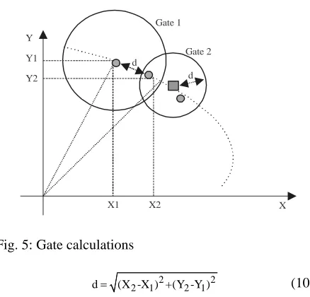
Selection of tracking gate: Ramachandra (2018), Richards et al. (2010) gating is a technique for eliminating unlikely observation-to-track pairings. A gate is formed around the predicted track position Fig. 5. In our project, we will use circular gate.

Gate calculations:

Initial first gate: We calculate the first gate from maximum target speed, we suppose it is equal (1000 m sec-1_{) and so, D/Δt = Max_Speed:}

Fig. 5: Gate calculations

(10)

2 2

2 1 2 1

d (X -X ) +(Y -Y )

where, Δt: the time between the first and second. Fig. 5.

Second gate: We calculate the diameter of this gate from tow target observations by calculation the distance between the mas Eq. 10 in Fig. 5:

Third gate: The gate size can be calculated from one of two methods: normalized statistical methods by Eq. 11 (Kolawole, 2003):

(11)

2 T -1

stat k k k

D y S y

None normalized statistical methods by Eq. 12:

(12)

2 2 2 2

stat m p m p scan

D (x -x ) +(y -y ) <(T ×Max_Speed)

Where:

: Residual vector between prediction and

y

measurement

S : Residual co-variance matrix

RESULTS AND DISCUSSION

Track and filter initiation techniques and simulation result: Track initiation is an important function of a tracking system. Essentially, a track initiator must be capable of starting or initiating a track whenever a new target appears in the scanned region. The initiation technique is logic-based. This method is summarized below (Konstantinova et al., 2003; Mahafza, 2000).

Initialize on the first two scans of the measurements and estimate the apparent. Velocity with every pair of the measurements. Let the velocity be denoted by Eq. 13:

(13) (2) (1)

(2)

j k

1

v = (r -r )

J. Eng. Applied Sci., 15 (2): 730-741, 2020

delay, z-1 x (n)0

x (n)s delay, z-1

T x (n)p

T

x (n)s .

Fig. 6: Effect of track initiation accuracy

If this expression satisfies the speed-gating criterion by Eq. 14:

(14) (2)

min max

v  v v

Then a track is initiated, so, predict the position the third scan as Eq. 15:

(15) (2)

(3) (2)

j

r (r Tv )

On the third scan, any measurement r_k(3) _{that falls}

within the gate will extend the initiated track. Next compute the velocity and acceleration as Eq. 16 and 17:

(16) (3) (2)

(3)

j k

1

v (r -r )

T



(17) (3) 1 (3) (2)

a (v -v )

T



Then, we use these (r, v, a) values to start tracking filter.

MATLAB simulation result: In Fig. 6, we see that when there is inaccurate filter initialization, the filter take more time (delay) to track the target.

Tracking algorithms and MATLAB results: Hanscom Air For Base, we will study some essential type of tracking filters and data association:

C (α-β) filter

C (α-β-γ) filter

C 2 state Kalman filter

C 3 state Kalman filter

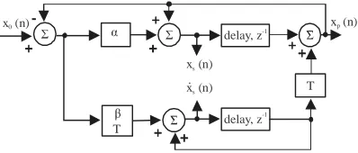
(α-β) filter: Duan et al. (2017), Mahafza (2000) this trackers are a widely used two-dimensional class of

Fig. 7: An implementation of (α-β) tracker

time-invariant filters and it is produces on the 9th observation smoothed estimates for position and velocity and a predicted position for the (n+l)th observation. The state module of this filter is given by Eq. 18-20 (Fig. 7): (18)

 

 

 



   



s p 0 p

x n = x n|n = x n + x n -x n

(19)

 

 

 



   



s s 0 p

x n = x' n|n = x n-1 + x n -x n

T



 

(20)

 





 

 

p s s s

x n = x n|n-1 = x n-1 +Tx n-1

where, on the (n) radar scans: α : Position gain factor β : Velocity gain factor T : Data interval xs (n) : Estimate position

xp (n) : Predicted position

: Estimate velocity

 

s

x n

σv

2 _{: Measured position}

Where the filter gain is (0< [α and β]<1). The filter coefficients can be chosen on the basic of a smoothing factor (ζ,) where (0 < ζ, <1) (Duan et al., 2017) as in Eq. 21:

(21)

 

2

2

=

=

1- 

 

In general, covariance matrix can be written as Eq. 22:

(22)

 

xx

C Cxx

C n|n =

C Cxx

 

 

  

  

The reduction of measurement noise is normally determined by the VRR ratios. This reduction ratio is the ratio of the output variance of the smoothed position estimate C_xx to the input measurement variance σ_v2 _as

follows in Eq. 23:

(23)





_

_

xx v x

2 -3 +2

VRR = C / =

42

-   

   10 20 30 40 50 60 70 80 90

Sample number

Real

and

est

emat

ed

po

si

tio

n

1.5

1.0

0.5

0.0 t-delay

Filter starting

J. Eng. Applied Sci., 15 (2): 730-741, 2020

Fig. 8: Maneuvering target with low smoothing factor ζ, = 0.1 (high gain)

Fig. 9: Maneuvering target with low smoothing factor ζ, = 0.9 (low gain) The velocity reduction variance ratio is measured as

the velocity estimation output given only the noise input as Eq. 24:

(24)





_

_

xx v

x 2

1 2

VRR = C / =

42 -T

 

  

  

MATLAB simulation results: In Fig. 8, we see that when we have low smooth factor, the estimated trajectory is not very fine but there is no a position off set.

In Fig. 9, we see that when we have high smooth factor, the estimated trajectory is very fine but there is an position offset.

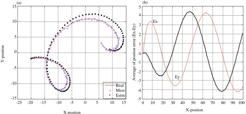
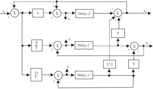
(α-β-γ) filter: Duan et al. (2017), Mahafza (2000) the (α-β-γ) tracker produces for the kth observation, smoothed

estimates of position, velocity and acceleration. It also produces the predicted position and velocity for the (K+l)th observation. The state module of this filter is given by Eq. 23-28 (Fig. 10):

(25)

 

 



   



s p 0 p

x n = x n + x n -x n

(26)

 

 

 



   



s s s 0 p

x n = x n-1 +Tx n-1 + x n -x n

T



  

(27)

 

 



   



s s ₂ 0 p

2

x n = x n-1 + x n -x n

T



 

(28)





 

 

 

p s s s

T

x n+1 = x n +Tx n + x n

2

 

15

10

5

0

-5

-10

-15

1.2

1.0

0.8

0.6

0.4

0.2

0.0

-0.2

(a) (b)

Y

-p

os

tio

n

A

v

erag

e of po

st

ion

erro

r (Ex-Ey

)

-25 -20 -15 -10 -5 0 5 10 15 X-position

0 10 20 30 40 50 60 70 80 90 100 Sample number

Ex

Ey

Real Mesr Estm

-25 -20 -15 -10 -5 0 5 10 15

X-postion X-postion

0 10 20 30 40 50 60 70 80 90 100 5

4

3

2

1

0

-1

-2

-3

-4

-5

A

v

erag

e of po

st

ion

erro

r (Ex-Ey

)

15

10

5

0

-5

-10

-15

Y

-p

os

tio

n

(a) (b)

Real Mesr Estm

Ex

J. Eng. Applied Sci., 15 (2): 730-741, 2020

x0 +

-+

+ _x

s

Delay, z-1

+ + +

xp

+ + T

xs

Delay, z-1

T

xp + +

T T /22

Delay, z-1 xs

+ +

γ

2 T2

Fig. 10: An implementation of (α-β-γ) tracker

Fig. 11: Maneuvering target with low smoothing factor ζ,= 0.1 (high gain) Where:

: Smoothed acceleration

 

s

x n



γ : Acceleration gain factor

Where the filter gain is (0< [α ,β, γ] <1). The filter coefficients can be chosen on the basic of a smoothing factor (ζ,) where (0<ζ, <1) as Eq. 29 (Duan et al., 2017):

(29) 3

2

3

1-1.5 (1- )(1- )

(1- )

  

   

  

A large smoothing when γ = 1 while γ = 0 means that no smoothing is present. A VRR ratio are computed is given by Eq. 30-32:

(30)







_

_





_



2

x

2 2 +2 -3 - 42

-VRR =

4-2 - 2 +2 -2

           

(31)















3 2 2

x 2

4 -4 +2

2-VRR =

T 4-2 - 2 + -2

    

    



(32)











2

x 4

4

VRR =

T 4-2 - 2 + -2



    



MATLAB simulation results: In Fig. 11, we see that when we have low smooth factor, the estimated trajectory is not very fine but there is no a position offset.

In Fig. 12, we see that when we have low smooth factor, the estimated trajectory is very fine but there is a position offset.

Kalman filter: Morrison (2012) Musicki et al. (2004) and Mahafza (2000) the Kalman filter is a linear recursive estimator that minimizes the mean squared error as long as the target dynamics are modeled accurately. Additionally, the Kalman filter has the following advantages (Sarkka, 2013).

15

10

5

0

-5

-10

-15

1.5

1.0

0.5

0.0

-0.5

-1.0 -20 -15 -10 -5 0 5 10 15

X position

0 10 20 30 40 50 60 70 80 90 100

Sample number

Y

p

os

it

ion

Av

era

g

e of

p

os

it

ion error

(Ex

.E

y)

(a) (b)

Real Mesr Estm

Ex

J. Eng. Applied Sci., 15 (2): 730-741, 2020

Time update Measurement update

1. State predictor:

2. Predictor of covariance matrix:

3. Kalman gain computation

4. State update

5. Covariance update (corrector equation) P (k+1/k) = Φk p (k/k) Φk+Qk

T

K (k) = P (k/k-1)G [G P (k/k-1)G +R ]k k k k+1

T T -1

P (k/k) = P (k/k-1)-k G P (k/k-1)k k x (k/k) = x (k/k-1)+K [y (k)-G x (k/k-1)]k k

^ ^ ^

^

x (k+1/k) = Φkx (k/k)

Fig. 12: Maneuvering target with low smoothing factor ζ,= 0.9 (low gain)

Fig. 13: Kalman filter algorithm

C The gain coefficients are computed dynamically. This means that the same filter can be used for a variety of maneuvering target environments

C The Kalman filter gain computation adapts to varying detection histories including missed detections

C The Kalman filter provides an accurate measure of the covariance matrix this allows for better implementation of the gating and association processes

C The Kalman filter makes it possible to partially compensate for the effects of miss-correlation and miss-association

Thus, the state prediction equation (for general case) is given by Eq. 33:

(33)

 

 

x (k+1) =Фk x k +Bk u k +Hk w(k)

Where:

Фk : Transition state matrix x (k) : The state at time k

u (k) : The known input or control signal w (k) : A sequence of zero-mean, white

Gaussian process noise with covariance Q and the measurement equation is given by Eq. 34:

(34)

 

   

y k = Gx k +v k

where, v (k) is a sequence of zero-mean, white, Gaussian process noise with covariance R, G measurement matrix. The random variables v (k) and w (k) represent the process and measurement noise, respectively. They are assumed to be independent (of each other), white and with normal probability distributions. Kalman filter steps are summarized in Fig.13.

There are two type of Kalman filter 2 state Kalman which consider the target as Constant Velocity (CV) and acceleration as external noise and 3 state Kalman which consider the target as Constant Acceleration (CA) and the variation in acceleration as external noise (Sarkka, 2013; Musicki et al., 2004).

MATLAB simulation results:

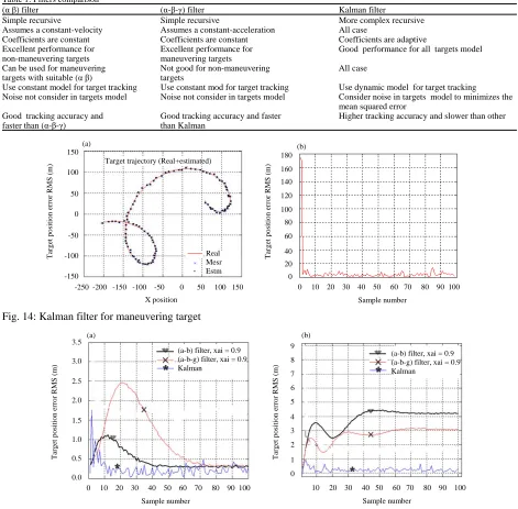
Filters comparison result: For the same maneuvering target trajectory and for non-maneuvering targets the filter comparison in the Table 1 and Fig. 14 and 15.

15

10

5

0

-5

-10

-15

3

2

1

0

-1

-2

-3

-4 -250 -200 -150 -100 -50 0 50 100 150

X position

0 10 20 30 40 50 60 70 80 90 100

Sample number

Y

p

os

it

ion

Av

era

g

e of

p

os

it

ion error

(Ex

.E

y

)

(a) (b)

Real Mesr Estm

Ex

J. Eng. Applied Sci., 15 (2): 730-741, 2020

Table 1: Filters comparison

(αβ) filter (α-β-γ) filter Kalman filter

Simple recursive Simple recursive More complex recursive

Assumes a constant-velocity Assumes a constant-acceleration All case

Coefficients are constant Coefficients are constant Coefficients are adaptive

Excellent performance for Excellent performance for Good performance for all targets model

non-maneuvering targets maneuvering targets

Can be used for maneuvering Not good for non-maneuvering All case

targets with suitable (αβ) targets

Use constant model for target tracking Use constant mod for target tracking Use dynamic model for target tracking

Noise not consider in targets model Noise not consider in targets model Consider noise in targets model to minimizes the

mean squared error

Good tracking accuracy and Good tracking accuracy and faster Higher tracking accuracy and slower than other

faster than (α-β-γ) than Kalman

Fig. 14: Kalman filter for maneuvering target

Fig. 15: Filters comparison

Data association algorithm (Konstantinova et al., 2003): In study, we talk about most popular algorithm called Global Nearest Neighbor Approach (GNNA) (Kolawole, 2003).

Algorithm descriptions: This method consist of three steps: We assume the existence of a set of n tracks (gates) at the time a new observation or set of observations is received. These observations may be used for updating the existing tracks or for initiating new tracks. Suppose that m measurements are received at time index k. In a cluttered environment, m does not necessarily equal n and it may be difficult to distinguish

whether a measurement originated from a target or from clutter. A validated measurement is one which is either inside or on the boundary of the validation gate of a target. We calculate the Cost [C_ij] matrix as following:

j

11 12 13 1m

ij 21 22 23 2m

n1 n2 n3 nm

1 2 3 ... m

1

c c c : c

2

C = c c c : c i

:

: : : : :

n

c c c : c

  _{ }      _{  }   _   _  _{ }      150 100 50 0 -50 -100 -150 180 160 140 120 100 80 60 40 20 0 -250 -200 -150 -100 -50 0 50 100 150

X position

0 10 20 30 40 50 60 70 80 90 100

Sample number Tar g et p os it ion erro r RMS (m ) Tar g et p os it ion erro r RMS (m )

(a) _(b)

Real Mesr Estm Target trajectory (Real+estimated)

3.5 3.0 2.5 2.0 1.5 1.0 0.5 0.0 9 8 7 6 5 4 3 2 1 0

0 10 20 30 40 50 60 70 80 90 100

Sample number

10 20 30 40 50 60 70 80 90 100

Sample number Tar g et p os it ion erro r RMS (m ) Tar g et p os it ion erro r RMS (m ) (a) (b)

(a-b) filter, xai = 0.9 (a-b-g) filter, xai = 0.9 Kalman

J. Eng. Applied Sci., 15 (2): 730-741, 2020

The elements of the Cost matrix cij have the

following values:

ij 2

ij

100 if measurement j is not in the gate of track i

c =

d if measurement j is in the gate of track i

  

About dij

2_{, tracking residual error (distance between}

center of gate i and the measurement j if measurement j is in the gate of the track i.

The desired solution of the assignment (cost) matrix is the one that minimizes the summed total distance. For simple cases the optimal solution can be easily found by enumeration. But the enumeration is too much time consuming in more complicated cases. We choose to solve the assignment problem by realizing the extension of Munkres (Hungarian) algorithm. As a result we yield the optimal measurements to tracks association. But it is possible (due to missed detection) that some track to be associated with measurement that is not a targets measurement.

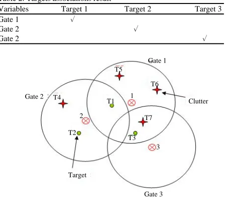
Algorithm example: Assume we have the track function as in Fig. 16. Calculate the distance between center of every gate i and its measurements j and form the cost matrix for example in gate 2:

Distance between T4 and center of this gate = 2.12 and then c24 = d24

2 _{= 4.48. T5 is out of this gate so}

c24 = 100 and so on. That we find the total cost matrix:

T1 T2 T3 T4 T5 T6 T7 2.25 100 6.25 100 4.48 4.48 2.89

C = 4.84 1 100 4.48 100 100 100

100 100 2.25 100 100 100 3.24

 

 

 

 

 

 

Find the optimal solution (lower cost) by using Munkres algorithm by MATLAB Software then

minimum cost value = c11+c22+c33 = 2.25+1+2.25 = 5.5

and it is mean that the data association will be as Table 2 and all other target will be canceled.

We see from Fig. 17 that 99% of false signal can be canceled by using this algorithms, so, this algorithm is useful for clutter cancelation in noisy environments.

Computer simulation results: Djerassi and Konstantinova (2002) now we built tracking simulation by VC++ to simulate all the previous algorithms. The simulation programs algorithm consist of next stages as follow, Fig. 18.

Targets generation: Drawing the targets trajectory and selecting its colors.

Table 2: Targets associations result

Variables Target 1 Target 2 Target 3

Gate 1 %

Gate 2 %

Gate 2 %

Fig. 16: Data association problems example

Fig. 17: MATLAB simulation

0 20 40 60 80 100 140

120

100

80

60

40

20

0

-20

-40

Y

pos

it

ion

X position

140

120 100

80

60

40

20

0

-20

-40

Y

pos

it

ion

140

120 100

80

60

40

20

0

-20

-40

Y

pos

it

ion

0 20 40 60 80 100 X position

0 20 40 60 80 100 X position False signal

False signal

(a) (b) (c) Gate 3 Target

Clutter Gate 1

Gate 2

3 T7

T3 1

T6 T5

T4

2

T2

J. Eng. Applied Sci., 15 (2): 730-741, 2020

Targets generation Scenario generation Adjust radar and f ilter parameter Start simulation

Select tracking f ilter Select scenario Select radar display option

Start simulation

Fig. 18: Tracking simulation flowchart

Fig. 19: Example of tracking simulation output

Scenario generation: By selecting multi targets from step 1 and determine the parameter for every target like (start time, start speed and acceleration) and save this scenario (we can generate unlimited number of scenario). Adjust the radar parameter: Like (PRF, Pulse Width, Scan Rate…).

Select tracking filter type: Alpha-beta, Kalman … and adjust the filter parameter.

Select the scenario: From scenario editor.

J. Eng. Applied Sci., 15 (2): 730-741, 2020

Fig. 20: Example of target simulation

Table 3: Filters comparison by simulation

Filter type Events Error-mean (m) Error-Rms (m) SD (m) Filter time cost (us)

(α-β) 49 358.40 485.76 327.89 1.77

(α-β-γ) 49 264.77 367.32 254.60 3.10

2 State-Kalman 49 211.27 279.44 182.90 4.70

3 State-Kalman 49 194.05 249.78 157.27 7.00

Start simulation: It is the main job of program which contains:

C Track initiation: calculate initial speed, gate and position

C Target tracking: draw the target position (prediction and estimation), target numbering and display targets information’s

C Draw target trajectory and give a report for all target with computer saving

C Calculate filter average-time and all tracking error Example for filters comparison by simulation: We select the target in Fig. 20 with start Speed = 300 m/sec, acceleration = 3 m/sec2 _{and R<100 km and computer is}

(COR I 3 with 4M_RAM).

Example of filter comparison by simulation: Table 3 are given below.

CONCLUSION

We studied the most important tracking algorithms like (αβ), (αβ γ) and Kalman filters and others. The choice of tracker depends on the complexity, accuracy and requirements of the mission. Kalman filter is suitable for all targets cases more than (αβ), (αβ γ) filters but more complex than the others and needs hi speed computer to use it. Data association algorithm (GNNA) is very important to solve targets association problem. Therefore by using this simulation we can add or

modify any algorithm and will help us to study any algorithm property and this simulation needs to add another algorithms to solve some tracking problem like maneuvering targets tracking detector or crossing target problem and in the next generation of this simulation we going to add more newest filters like Extended Kalman Filter (EKF), Particles Filter (PF). This simulation is very useful for any one wants to learn target tracking or wants to work in radar station because it gives him a real work like real radar. Finally, this simulation can be easley modified to work as real tracking radar by inject real data from radar receiver to computer (with synchronal signal) by any computer interface hard-ware like USB, RS485 or PCI acquisition card.

REFERENCES

Djerassi, E. and P. Konstantinova, 2002. Object-oriented environment for assessing tracking algorithms. Inf. Secur., 9: 93-106.

Duan, Y., X.S. Tan, Z.G. Qu, H. Wang and J. Wang, 2017. Adaptive tracking gate design for maneuvering target in clutter environment. Proccedings of the 2017 IEEE 2nd International Conference on Information Technology, Networking, Electronic and Automation Control (ITNEC’17), December 15-17, 2017, IEEE, Chengdu, China, pp: 1449-1455.

Kolawole, M.O., 2003. Radar Systems, Peak Detection and Tracking. Elsevier, Oxford, UK.

1

2 3

J. Eng. Applied Sci., 15 (2): 730-741, 2020

Konstantinova, P., A. Udvarev and T. Semerdjiev, 2003. A study of a target tracking algorithm using global nearest neighbor approach. Proceedings of the International Conference on Computer Systems and Technologies (CompSysTech’03), June 19-20, 2003, Rousse, Bulgaria, pp: 290-295.

Mahafza, B.R., 2000. Radar Systems Analysis and Design Using MATLAB. Chapman and Hall/CRC, Ney York.

Morrison, N., 2012. Tracking Filter Engineering: The Gauss-Newton and Polynomial Filters. Institution of Engineering and Technology, Stevenage, England, ISBN: 9781849195553, Pages: 577.

Ramachandra, K.V., 2018. Kalman Filtering Techniques for Radar Tracking. 1st Edn., CRC Press, Boca Raton, Florida, USA., ISBN: 9780824793227, Pages: 256.

Richards, M.A., W.A. Holm and J. Scheer, 2010. Principles of Modern Radar: Basic Principles. Institution of Engineering and Technology, Stevenage, England, ISBN: 9781891121524, Pages: 960.