Original citation:
Sinanan, S. K. and Holt, D. F.. (2016) Algorithms for polycyclic-by-finite groups. Journal
of Symbolic Computation. doi: 10.1016/j.jsc.2016.02.008
Permanent WRAP url:
http://wrap.warwick.ac.uk/77143/
Copyright and reuse:
The Warwick Research Archive Portal (WRAP) makes this work by researchers of the
University of Warwick available open access under the following conditions. Copyright ©
and all moral rights to the version of the paper presented here belong to the individual
author(s) and/or other copyright owners. To the extent reasonable and practicable the
material made available in WRAP has been checked for eligibility before being made
available.
Copies of full items can be used for personal research or study, educational, or
not-for-profit purposes without prior permission or charge. Provided that the authors, title and
full bibliographic details are credited, a hyperlink and/or URL is given for the original
metadata page and the content is not changed in any way.
Publisher’s statement:
© 2016, Elsevier. Licensed under the Creative Commons
Attribution-NonCommercial-NoDerivatives 4.0 International
http://creativecommons.org/licenses/by-nc-nd/4.0/
A note on versions:
The version presented here may differ from the published version or, version of record, if
you wish to cite this item you are advised to consult the publisher’s version. Please see
the ‘permanent WRAP url’ above for details on accessing the published version and note
that access may require a subscription.
Algorithms for Polycyclic-by-Finite Groups
IS.K. Sinananb,˚, D.F. Holta
aMathematics Institute, University of Warwick, Coventry CV4 7AL, United Kingdom bDepartment of Mathematics and Statistics, University of The West Indies, Saint
Augustine, Trinidad and Tobago
Abstract
A set of fundamental algorithms for computing with polycyclic-by-finite groups is presented.
Polycyclic-by-finite groups arise naturally in a number of contexts; for ex-ample, as automorphism groups of large finite soluble groups, as quotients of finitely presented groups, and as extensions of modules by groups. No existing mode of representation is suitable for these groups, since they will typically not have a convenient faithful permutation representation.
A mixed mode is used to represent elements of such a group, utilising either a power-conjugate presentation or a polycyclic presentation for the elements of the normal subgroup, and a permutation representation for the elements of the quotient.
Keywords: polycyclic, polycyclic-by-finite, permutation, finitely presented, magma
1. Introduction
A group is polycyclic-by-finite if it has a normal polycyclic subgroup of fi-nite index. That is, if it has a normal subgroup of fifi-nite index that admits a subnormal series with cyclic factors.
By a well-known theorem of P. Hall, every polycyclic-by-finite group is finitely presented — and in fact, polycyclic-by-finite groups form the largest known section-closed class of finitely presented groups. It is this fact that makes
IThis research was supported by the University of Warwick Postgraduate Research
Schol-arship, and the University of Warwick Chancellor’s International ScholSchol-arship, which are, in turn, funded partly by the Engineering and Physical Sciences Research Council of the United Kingdom (EPSRC).
˚Corresponding author
Email addresses: [email protected](S.K. Sinanan), [email protected](D.F. Holt)
URL:https://sta.uwi.edu/fst/dms/Shavak_Sinanan.asp(S.K. Sinanan),
polycyclic-by-finite groups natural objects of study from the algorithmic stand-point.
The algorithmic decision theory of polycyclic-by-finite groups has been in-vestigated in the theoretical context by Baumslag et al. (1991). However, from the computational standpoint, the algorithms presented by Baumslag et al. (1991) are not applicable, nor were they intended to be. In contrast, this paper explores the computational properties of polycyclic-by-finite groups from a prac-tical perspective, detailing algorithms which lend themselves easily to computer implementation.
Specifically, the work presented in this paper aims to:
(a) Define a computationally effective representation for polycyclic-by-finite groups.
(b) Develop a set of implementable algorithms to perform fundamental compu-tations such as element multiplication and subgroup construction, within the class of polycyclic-by-finite groups.
(c) Use the fundamental algorithms developed to design methods that perform more advanced computations such as the construction of centralisers and conjugacy testing, within the class of polycyclic-by-finite groups.
The algorithms presented here are targeted primarily at finite non-solvable groups with a large solvable (and hence, in this case, polycyclic) normal sub-group, as such groups often do not have a convenient permutation representa-tion. Groups of this type arise naturally in many applications, such as automor-phism groups of large finite solvable groups, as quotients of finitely presented groups, and as extensions of modules by groups.
The theory developed is by no means limited to the finite case. Apart from a few natural exceptions (such as computing Sylow subgroups), all of the algorithms apply equally to infinite polycyclic-by-finite groups.
Whilst there may be many different decompositions of a given polycyclic-by-finite group as an extension of a polycyclic group by a finite group, the algorithms presented in this paper are most useful for those decompositions in which the finite quotient admits a faithful permutation representation of manageable degree (ă 106). Thus, it will hereinafter be assumed that the polycyclic-by-finite groups in question can be so decomposed.
Much of what is presented in the sequel requires familiarity with the already existing efficient algorithms for computing with finite permutation groups, and with polycyclic groups. The standard references for computation with permu-tation groups are (Sims, 1970, 1971), and (Seress, 2003). The nopermu-tation used in this paper is consistent with the latter.
LetE be a polycyclic-by-finite group, and suppose that there is a black-box representation of E on the computer. Let N IJ E be polycyclic, and assume that G “ E{N admits a faithful permutation representation of manageable degree. Concretely, the central goal of the theory is to set up machinery so that elements ofEcan be manipulated by performing operations only withinN and
G, without appealing to the existing representation of E.
On the other hand, although the algorithms described here are designed for situations where one is unable to perform arithmetic inE, there may neverthe-less be instances in which it would be efficient to be able to do this; and similar methods to those presented here may be applied to such groups. This happens, for example, in dealing with some types of large matrix groups over finite fields as described in (Hulpke, 2013).
2. Multiplication
This section contains a detailed description of a mode by which elements of a given polycyclic-by-finite group may be represented on the computer, and a strategy for multiplication of elements represented in this manner.
Fix a transversalL ofN in E with 1E PL and, forePE, denote byethe
unique element ofeNXL. An elementePE can of course be written uniquely as a producte“e¨n, wherenPN.
Note. For ease of notation, in what follows, the elementePLwill be identified with the element eN of the quotient G; the context will be made explicit in cases where it is not clear.
Expressing group elements in this manner is a logical approach as one would naturally wish to utilise the well-developed algorithms available for the classes of permutation groups and polycyclic groups, thereby fully exploiting the structure of the group in question.
In what follows it is assumed that the normal subgroup N ofE is defined by a polycyclic presentation, although the methods described can be extended to different representations ofN.
2.1. Bases and Strong Generating Sets
The definitions given in (Seress, 2003, ch. 4) for a base and a strong gener-ating set may be extended to fit the context of polycyclic-by-finite groups.
View G as a permutation group of degree d and denote by Ω the set of points on which G acts. Given an element en P E and a point ω P Ω one may unambiguously speak of the action ofenonω, with obvious meaning, viz.
ωen
“ωe; regardingeas an element ofG.
A sequence B“ pγ1, . . . , γkqof elements belonging to Ω is called abase for
E if every element ofE that fixes B pointwise belongs toN. The sequenceB
defines a stabiliser subgroup chain
E“Er1sěEr2sě ¨ ¨ ¨ ěErksěErk`1s“N (2.1)
where Eris “E
pγ1,...,γi´1q (i ą1) is the pointwise stabiliser of tγ1, . . . , γi´1u. The base B is called non-redundant if Eri`1s ăEris for all i “1, . . . , k. The
orbits γiE
ris
are called the basic orbits or fundamental orbits of E (relative to
B). The subgroupEris is called thei-th basic stabiliser relative toB. Astrong generating set forE relative toB is a generating setT forE with the property that
xTXEris
y “Eris (2.2)
fori“1, . . . , k`1. One has
|G| “
k
ź
i“1
rEris{N:Eri`1s{N
s.
By the Third Isomorphism Theorem and the Orbit–Stabiliser Theorem, one obtains rEris{N : Eri`1s{Ns “ |γEris
i | ďd for i “ 1, . . . , k. Moreover, if B is
non-redundant, then rEris{N : Eri`1s{Ns ě 2 for each i. These inequalities,
combined with the expression for|G|above, yield
log2|G|
log2d ď |B| ďlog2|G|. (2.3)
2.2. The Normal Form
A base and strong generating set data structure for the permutation groupG
combined with a power-conjugate or polycyclic presentation forNautomatically induce a normal form for elements ofE. The existence of a normal form for group elements allows one to devise a multiplication strategy which is suitable for computer implementation.
Let S “ tx1, . . . , xmu be a strong generating set relative to a base B “
pβ1, . . . , βlqforG, and assume thatS is non-redundant. Denote byS´1the set
tx´1
1 , . . . , x´ 1
mu. For technical reasons, the transversalLis constructed so that,
for eachxPS which is not self-inverse inG, one hasx´1 =x´1.
For eachi, denote thei-th basic stabiliser relative toB byGris, and denote
the i-th basic orbit relative to B by ∆i “ tδi,1, . . . , δi,diu, where δi,1 “ βi. LetUi be a right transversal of Gri`1s in Gris; then each element ofG can be
represented uniquely as a product of transversal elementsul¨ul´1¨ ¨ ¨u1 where
uiPUi.
Additionally, let Si “ SXGris “ txi,1, . . . , xi,siu and denote by S
´1
i the
settx´i,11, . . . , x´i,s1
a Schreier vector — see (Seress, 2003)), and that this data structure remains unchanged throughout the operation of the method.
An element e P E may be expressed as ul¨ul´1¨ ¨ ¨u1¨n1 where ui P Ui.
Consider multiplying the elementseandx¨n2(wherexPSYS´1andn2PN):
ul¨ul´1¨ ¨ ¨u1¨n1¨x¨n2“ul¨ul´1¨ ¨ ¨u1¨x¨nx1¨n2.
In this setup, the multiplication algorithm should possess the following func-tionality:
(i) Conjugate elements ofN by elementsxPSYS´1.
(ii) Rewrite an expression of the form ul¨ul´1¨ ¨ ¨u1¨xas u1l¨u1l´1¨ ¨ ¨u11¨n whereu1
iPUi andnPN.
Utilising the existing representation of N, items (i) and (ii) are sufficient to formulate a strategy by which arbitrary elements of E may be multiplied without appealing to the existing representation ofE. The details of how this is accomplished are given in Subsections 2.3–2.4.
2.3. The Shifting Method
Fixiand j, and letuPUi be the permutation taking βi to δi,j P∆i. Take
xP Si, and let h, h1 be the permutations in Ui which map βi to βiu¨x “δ x i,j,
βu¨x´1
i “δx
´1
i,j respectively. Then, in the groupE, one has
u¨x“y1y2¨ ¨ ¨yk¨h¨n, (2.4a)
u¨x´1“z
1z2¨ ¨ ¨zk1¨h1¨n1, (2.4b)
for somen, n1PN, and where y
1, . . . , yk, z1, . . . , zk1PSi`1YSi´1
`1.
The elements n and n1 are called the heads of u relative to x and x´1 respectively while the wordsy1y2¨ ¨ ¨yk andz1z2¨ ¨ ¨zk1 are called thetails ofu relative toxandx´1respectively. Equations (2.4) are called theshift equations. Note that there areOpd|B||S|qshift equations.
The shift equations suggest a scheme by which elements ofE may be mul-tiplied. Assume that the tails can be computed consistently for each pairu, x, andu, x´1 of the shift equations. Furthermore, assume that the conjugates of elements ofN by elements ofSYS´1 can be calculated without appealing to the existing representation ofE.
Lete1“e1n1ande2“e2n2be two elements ofEin normal form. Using the methods available for permutation groups, the algorithm begins by writinge1as
ulul´1¨ ¨ ¨u1, whereuiPUi for eachi, and expressese2as a word overSYS´1, say w “ q1q2¨ ¨ ¨qσ where qj P S YS´1 for each j. (Note that the existing
methods available for permutation groups allow one to do this consistently.) The algorithm then proceeds to rearrange the terms of the product by con-jugating the elementn1 by the wordw, as illustrated in Equation (2.5):
e1¨e2“ pulul´1¨ ¨ ¨u1q ¨n1¨ pq1q2¨ ¨ ¨qσq ¨n2
The under-bracketed segment of Equation (2.5) can be recognised as the left-hand side of a shift equation, sayu1¨q1“y1y2¨ ¨ ¨yκ¨h1¨n3for some n3PN,
h1 P U1, and where yj P S2 YS2´1 for each j. Via direct substitution, this equation can be used toshift the transversal elementq1pastu1. The algorithm executes this shifting procedure as illustrated in Equation (2.6).
e1¨e2“ulul´1¨ ¨ ¨u2u1¨q1
loomoon
replace byy1y2¨¨¨yκ¨h1¨n3
q2¨ ¨ ¨qσ¨nw1n2
“ulul´1¨ ¨ ¨u2¨y1y2¨ ¨ ¨yκ¨h1¨q2q3¨ ¨ ¨qσ¨nq1
´1w
3 n
w
1n2
(2.6)
The under-bracketed segment of the product in Equation (2.6) can again be recognised as the left-hand side of a shift equation. The algorithm repeats the procedure above to shiftq2 pasth1.
Remark 2.1. Each time a shift is made, the word overSYS´1 immediately to the left of the sequence of normal subgroup elements in the expression for the product is reduced by exactly one symbol.
The algorithm continues iterating through the wordw, shifting at every step, arriving at an expression of the form ulul´1¨ ¨ ¨u2¨y1y2¨ ¨ ¨yζ ¨u11¨n1 for the product, whereu1
1PU1, n1PN.
At this stage, the algorithm has decreased the sequence of transversal ele-mentsui on the right-hand side of Equation (2.5) by one term, thus reducing
the problem to a smaller case. The algorithm restarts its inner loop to process the wordy1y2¨ ¨ ¨yζ by, as before, recognisingu2¨y1 as the left-hand side of a shift equation.
Remark 2.2. Each time a word over SYS´1 is processed fully as described above, the leftmost sequence of transversal elementsuiin the expression for the
product is decreased by exactly one term.
Remark 2.3. Whenever a shift is made at leveli(with respect to the base and strong generating set hierarchy), the elements ofSYS´1that are placed to the left of the new element,hi(wherehiPUi), belong toSi`1YSi´`11. In particular, sinceSl`1“ H, no non-trivial elements ofSYS´1 are placed to the left of an element ofUl.
The word-processing procedure is repeated for each ui, after which a series
of conjugations of elements of the normal subgroup is performed. This yields an expression of the formu1
lu1l´1¨ ¨ ¨u11 ¨n2 for the product, wheren2PN, and
u1
iPUi for eachi.
Remark 2.4. The shift equations (2.4), together with the conjugation equations
nx=xnx forx
2.4. The Multiplication Algorithm
The multiplication algorithm relies directly on a precomputed set of data to facilitate its execution. More specifically, the following data is computed (using the existing representation ofE) on initialisation and held in memory.
(i) The tail of each shift equation. This computation takes place entirely within the permutation group. Assuming (henceforth) that a Schreier vector data structure is used, the storage required isOp|S|pd|B|q2q, where
dis the degree of the permutation groupG.
(ii) The head of each shift equation. This computation uses the existing rep-resentation of E and requires Opdr|B||S|qstorage, where r is the length of the polycyclic sequence used to defineN.
(iii) For each polycyclic generatoraofN, and eachyPSYS´1, the conjugate
ay. The memory requirement here isOpr2|S|
q.
The multiplication method is presented in Algorithm 1. The notation em-ployed thus far is used in the pseudocode, and the method assumes that the tails of the shift equations are stored as arrays of strong generators. The method also assumes the existence of a functionLengthwhich, when supplied with an ar-ray (or a sequence), returns the number of non-null entries of that arar-ray (or sequence).
Theorem 2.5. The multiplication algorithm terminates with the correct value for the desired product.
Proof. Termination is guaranteed by Remarks 2.1–2.3, while Equations (2.5) and (2.6) imply correctness.
The running time of Multiply is determined by the number of times that Lines 13–19 are executed. To estimate this number, an upper bound for
Length(rightword) will be established (for each of thel iterations of the outer
loop).
The rate of growth ofrightwordis investigated as follows. Initially,rightword
has length at mostd|B|. Each shift made in the inner loop of the algorithm appends a tail of length at mostd|B| to the variableleftword. This operation is performed in Line 15. Since a shift is made for each element of rightword, it follows that, at the end of the first iteration of the outer loop, leftword has lengthď pd|B|q2; and so, in the second iteration of the outer loop, rightword
has lengthď pd|B|q2. Repeating this argument shows thatrightwordhas length
ď pd|B|qi in thei-th iteration of the outer loop. Thus, in a run of Multiply,
Lines 13–19 are executedď
|B|
ř
i“1
pd|B|qiPO`pd|B|q|B|˘times.
The most expensive computations within Lines 13–19 occur in Line 16 and in Line 18. Line 16 consists of an application of a straightforward iterative procedure to compute the conjugate of an element ofN by an element of SY S´1 using the precomputed data set. Therefore, in a single run,
Multiply
Algorithm 1Element multiplication
1: functionMultiply(e1n1,e2n2)
2: if e2 is trivialthen
3: returne1n1n2
4: Writee1 in normal formulul´1¨ ¨ ¨u1 whereui PUi for eachi
5: Writee2 as a wordw“q1q2¨ ¨ ¨qtwhereqiPSYS´1for eachi
6: rightword Ð[q1,q2, . . . ,qt],leftwordÐ[]
7: n1
1Ðn1
8: foriÐ2to l do 9: n1
iÐ1N
10: foriÐ1to l do 11: u1
i Ðui
12: forjÐ1to Length(rightword)do
13: Retrieve from memory the tail array,tailword, and head,nσ, of
14: the shift equation corresponding to the pair u1
i,rightword[j]
15: leftword Ðleftwordcattailword
16: Find the conjugatenγ ofn1i byrightword[j] ŹUse the data set
17: n1iÐnσ¨nγ
18: FindhPUiwhich mapsβ u1
i
i to the image ofβ u1
i
i underrightword[j]
19: u1
iÐh
20: rightwordÐleftword 21: leftwordÐ[]
22: e˚ Ð1G,n˚Ð1N, iÐl
23: while ią0do 24: n˚Ðn
u1 i
˚ ¨n1i,e˚ Ðe˚¨u1i ŹUse the data set
25: iÐi´1
26: n˚ Ðn˚¨n2
computation inGwhich requiresOpdqmultiplications in the finite quotientG; for a proof of this, (see Seress, 2003, ch. 4). Thus, a run ofMultiply requires
O`dpd|B|q|B|˘multiplications inG.
In light of the exponential growth of the words through which Multiply
must iterate, small-base representations for the quotient group are desirable for satisfactory performance of the multiplication algorithm.
2.5. Applications
There are several immediate applications of the multiplication procedure.
(i) Giveng PG, compute the representative ofg in L in normal form. The way that this is done depends on the data structure used to represent the transversals in G; if a Schreier vector is used, then the representative is found by multiplying through the sequence inSYS´1 encodingg. (ii) Givene“en1 written in normal form, computee´1 in normal form. To
do this, first use the method in (i) to compute the representative ofe´1 (regarded as an element ofG) inL, saye´1n
2. Thenen1¨e´1n2“n3for somen3PNwhich can be computed usingMultiply. Therefore, one has
e´1 “ pe´1n
2q ¨n´31. Assuming that Schreier vectors are used to encode transversal elements, finding the inverse of an element inE requiresOpdq
multiplications.
(iii) Compute the order of e“en. First utilise the existing methods for per-mutation groups to compute the order of eregarded as an element ofG. Then use Multiply to raiseento this power. This yields an element of
N whose order can be computed using the existing methods for polycyclic groups; the order ofenis of course the product of the two numbers.
3. Transfer to the Category of Polycyclic Groups
Outlined in this brief section is a method that computes a consistent power-conjugate (or polycyclic) presentation for a polycyclic-by-finite groupE that is in fact polycyclic. For the sake of clarity, it will be assumed in the following discussion that E is finite, and a power-conjugate presentation for E will be constructed; a similar procedure may be employed in the infinite case.
Continuing with the notation from previous sections, ifEis polycyclic, then the quotient G “ E{N is polycyclic and one may use the already available methods for permutation groups to compute a power-conjugate presentation for G (see Seress, 2003, ch. 7). A consistent polycyclic or power-conjugate presentation forE may be found by “glueing together” the presentations forG
andN as described below.
LetN and Ghave consistent power-conjugate presentations
xa1, . . . , ar|a pj
j “wj,j for 1ďj ďr, ajai“wi,j for 1ďiăjďry,
and
xb1, . . . , bs|bj qj
“vj,j for 1ďjďs, bj bi
respectively, where
(i) pj, qj are the least primes such that a pj
j P xaj`1, . . . , ary for j ă r and
bj qj
P xbj`1, . . . , bsy for j ăs, and aprr, bs qs
are the identity elements in
N,Grespectively, and
(ii) wi,j, vi,j are words in the generator setstai`1, . . . , aru, tbi`1, . . . , bsu
re-spectively.
A power-conjugate presentation forEcan be constructed on the set of gener-atorstb1, . . . , bs, a1, . . . , aruas follows. First, regard the elementsbj as elements
ofE(the normal form of each of these elements may be obtained using the pro-cedure outlined in Subsection 2.5); one hasbj
qj
“vj,jn1 for somen1 PN. The
power-conjugate presentation forN may be used to expressn1as a word in the
required form over its polycyclic generators. Power relations with left-hand-side
apj
j remain unchanged in the new presentation.
Conjugate relations are derived in a similar manner; the multiplication algo-rithm is partly utilised to conjugate the elementsaj according to the hierarchy
induced by G and N. The presentation so obtained is a consistent power-conjugate presentation forE.
4. The Extended Schreier–Sims Algorithm
The class of polycyclic-by-finite groups is of course closed under the forma-tion of subgroups, and so, it is theoretically possible to represent subgroups using the scheme described in Section 2.
Using the notation of 2, the problem of representing subgroups may be for-mulated more concretely as follows. Given a set of generators, written in normal form relative toGandN, of a subgroupH ďE it is required to compute the following information relating toH:
(i) The normal polycyclic subgroupNH“HXN ofH.
(ii) A baseBH and strong generating set T relative to BH, for the quotient
GH“H{NH–HN{N.
(iii) Elements of Erepresenting images ofT in a transversalLH ofNH in H.
(iv) Conjugates of each polycyclic generator ofNH by the images ofT in LH.
(v) Data corresponding to Equations (2.4) in the context ofH.
Items (iv) and (v) are calculated in a manner similar to that of the parent group.
The difficulty lies in computing (i) and (iii). The approach taken is to ex-tend the well-known Schreier–Sims method described in (Seress, 2003, ch. 4), to efficiently compute the segments of data described in (i), (ii), and (iii) si-multaneously. Given a set of elements of E that generate a subgroupH ďE
In the language of the definitions made in Subsection 2.1, the chief objective of the Extended Schreier–Sims method may be stated more simply: given a set of generators of a subgroupH ď E the method attempts to compute a base and a strong generating set forH.
4.1. The Sifting Procedure
Before turning to the problem of how a base and a strong generating set for a subgroup of a polycyclic-by-finite group are computed, it will be assumed for the moment that these are given, and a version of thesifting (see Seress, 2003, ch. 4) procedure for polycyclic-by-finite groups will be introduced.
LetSH be a strong generating set for the subgroupH ofE, with associated
base BH “ pγ1, . . . , γkq. Assume that the basic orbits Θi “γiH
ris
have been calculated and that Schreier vectors encoding right transversalsRi ofHri`1s in
Hrisexist for eachi, with elements ofR
irepresented as products overSHXHris.
The sifting algorithm operates as follows. GivenenPE and jP t1, . . . , ku, the algorithm attempts to find the coset representative y1n11 P Rj such that
γen j “γ
y1n11
j , and (if j ăk) computese2n2“en¨ py1n11q´1 PHrj`1s if a coset representative is found. If no such coset representative exists, thenentakesγj
out of the orbit Θj, and the algorithm breaks and returns the siftee enalong
with an integer indicating the point at which the break occurred (in this case
j). Otherwise, the algorithm continues and attempts find y2n12 P Rj`1 such thatγe2n2
j`1 “γ
y2n12
2 and then computese3n3“e2n2¨ py2n12q´1 if possible. The algorithm attempts to perform k´j`1 iterations of this type, immediately breaking if, at any stage, the base point is taken out of orbit, in which case the siftee and an integer indicating the stage is returned. If the algorithm is able to perform all iterations successfully, then it returns the siftee and the integer
k`1.
Remark 4.1. The elementenPE belongs toH if and only ifk´j`1 iterations are performed by the sifting procedure, and the siftee returned belongs toHXN. Thus, the sifting algorithm has reduced membership testing inHto membership testing inH XN, which can be accomplished using the available methods for polycyclic groups (see Holt et al., 2005, sec. 8.3).
The sifting procedure is presented in Algorithm 2. The function operates as described above, taking as input an elementenof a polycyclic-by-finite group
E, a baseBH for a subgroup H ďE, the sequence Θ“ pΘ1, . . . ,Θkqof basic
orbits, a sequenceR“ pR1, . . . , RkqwhereRiis a transversal ofHri`1s inHris,
Algorithm 2Sifting
1: functionSift(en,BH, Θ,R,j)
2: kÐLength(BH)
3: esnsÐen
4: foriÐj to kdo Źesns fixes base pointsγ1, . . . , γi´1
5: ωÐγesns
i
6: if ωRΘi then
7: returnesns,i
8: Find the coset representativeyin1iPRi such thatγ yin1i
i “ω
9: esnsÐesns¨ pyin1iq´1
10: returnesns,k`1
Assuming that the transversals are encoded as Schreier vectors,Siftrequires
Opdkqmultiplications inE, where kis the length of the input base.
4.2. Extending the Schreier–Sims Algorithm
The operation of the extended Schreier–Sims algorithm is based on the fol-lowing lemma, whose proof is a straightforward induction on the base length.
Lemma 4.2. Let E be a polycyclic-by-finite group,H ďE and let N ŸE be polycyclic of finite index inE. Assume that there is a known permutation rep-resentation for the quotientG“E{N, and that the elements ofE are expressed in normal form relative toGandN. Denote the set on whichGacts by Ωand lettγ1, . . . , γku ĎΩ. For eachi in t1, . . . , k`1u, let SH,iĎHpγ1,...,γi´1q such
thatxSH,iy ě xSH,i`1y holds foriďk. IfH “ xSH,1y,SH,k`1ĎHXN, and
xSH,iyγi “ xSH,i`1y (4.1)
holds for each i, then BH “ pγ1, . . . , γkq is a base for H andSH “
Ťk`1
i“1 SH,i
is a strong generating set forH relative to BH.
Given a setX of generators for a subgroup H ďE the extended Schreier– Sims algorithm constructs a base and strong generating set in the following way. A data structure containing a listBH“ pγ1, . . . , γkqof already known elements
of a non-redundant base is maintained, along with an approximationSH,ifor a
generator set of the stabiliserHpγ1,...,γi´1qfor eachiP t1, . . . , k`1u. Throughout execution, theSH,i satisfy the property that, for all i, xSH,iy ě xSH,i`1y, and
SH,k`1 Ď HXN. The data structure is said to be up-to-date below level j if Equation (4.1) holds for eachiin the rangejăiďk.
In the case where the data structure is up-to-date below levelj, a transversal
Rj of xSH,jyγj in xSH,jy is computed. Then a check is made to determine
whether Equation (4.1) is satisfied for i“j. This can be done by sifting the Schreier generators (see Seress, 2003, ch. 4) obtained fromRj andSH,j in the
group xSH,j`1y. By Remark 4.1, membership testing is possible in the group,
xSH,j`1y, since Lemma 4.2 implies thatŤ
k`1
for xSH,j`1y relative to the base pγj`1, . . . , γkq. If all Schreier generators are
inxSH,j`1ythen the data structure is up-to-date below levelj´1. Otherwise there exists a non-trivial sifteeesnswhich takes some base point, sayγt, out of
orbit. Ift“k`1 andes‰1G, then a new base pointγk`1is appended toBH
from supppesnsqand the set SH,k`2 is initialised with the contents of SH,k`1. The sifteeesnsis added to the sets SH,j`1, . . . , SH,t, and the data structure is
now up-to-date below level minpt,|BH|q.
The algorithm initialisesBH to contain a sequence of pointsγ1, . . . , γk in Ω
such that each point is moved by at least one generator inX with non-trivial first component, and setsSH,itoXX xXypγ1,...,γi´1qfori“1, . . . , k`1. At that
moment, the data structure is up-to-date below levelk; the algorithm terminates when the data structure becomes up-to-date above level 0.
A simplified version of the extended Schreier–Sims method is presented in Algorithm 3. The function takes as input a setXof elements of a polycyclic-by-finite groupE and operates as described above to compute a base and strong generating set forH “ xXy.
The notation employed thus far is used in the pseudocode, and
SuperSchreierSimsalso assumes the existence of a procedureAppendwhich, when supplied with an array (or sequence) and an element, appends the element to the end of the array (or sequence).
The normal subgroup HXN ofH can be computed easily from the strong generating setSH returned bySuperSchreierSims as it is generated by the
elements inSH with trivial first component.
Theorem 4.3. The extended Schreier–Sims method terminates, returning a correct base and strong generating set.
Proof. This is immediate from Lemma 4.2 and the discussion following it.
The dominant computations inSuperSchreierSimsare the multiplications in E using the normal form for elements, and these multiplications occur in Lines 18, 20, 21, and 25. Lines 18, 20, and 21 each requireOpdqmultiplications; and, with an application of (2.3), one sees that Line 25 requires Opdlog|G|q
multiplications.
In practice, when a new loop is commenced in Line 16 only Schreier genera-tors which have not been previously checked are constructed (Lines 18, 20, and 21) and sifted (Line 25). Therefore, the lines in question are executed exactly once for each Schreier generator.
After initialisation in Lines 3–11, eachRi has size at mostd, and eachSH,i
has size at most|X|. By (2.3), the number of Schreier generators before any sift operations are performed isOpd|X|log|G|q.
Observe that although the setsRi andSH,ichange during the operation of
the algorithm, they are always only augmented, and therefore, elements ofRi
and SH,i are be combined to form a Schreier generator only once. Fix i and
set K “ xSH,iy; every time the setSH,i is augmented, the group KN{N ďG
Algorithm 3The extended Schreier–Sims algorithm
1: functionSuperSchreierSims(X)
2: BHÐ pq,kÐ0
3: forenPX do
4: if e‰1G and γien“γi @ iP t1, . . . , kuthen Źenfixes all points
inBH
5: Findγk`1PΩ withγken`1‰γk`1
6: Append(BH, γk`1)
7: kÐk`1
8: foriÐ1to kdo
9: SH,iÐ tenPX|γjen“γj @jP t1, . . . , i´1uu
10: HrisÐ xS
H,iy, ΘiÐγH
ris
i ,
11: Compute a stabiliser transversalRi inHris corresponding to Θi
12: ΘÐ pΘ1, . . . ,Θkq, RÐ pR1, . . . , Rkq
13: SH,k`1Ð tenPX|e“1Gu
14: NH Ð xSH,k`1y ŹThis subgroup is generated inN
15: iÐk
16: while iě1do 17: forθPΘi do
18: Find the coset representativeenPRi such that γien“θ
19: forxnxPSH,ido
20: Find the coset representativee1n1PR
i such thatγe
1n1
i “θxnx
21: enÐen¨xnx¨ pe1n1q´1
22: if en“1 then
23: continue xnx
24: uptodateÐtrue
25: en,j ÐSift(en,BH, Θ,R,i`1)
26: if e‰1G then
27: uptodateÐfalse 28: if jąkthen
29: Findγk`1PΩ withγken`1‰γk`1
30: Append(BH,γk`1) ŹExtend base
31: kÐk`1
32: SH,k`1ÐSH,k ŹMaintain inclusion
33: else if nRNH then
34: uptodateÐfalse
35: SH,kÐSH,kY tenu,NHÐ xNH, ny
36: jÐk
37: if not uptodatethen 38: fortÐi`1 to j do
39: SH,tÐSH,tY tenu,HrtsÐ xSH,ty, ΘtÐγH
rts
t ,
40: Compute a stabiliser transversalRtin Hrts
42: ΘÐ pΘ1, . . . ,Θkq,RÐ pR1, . . . , Rkq
43: iÐj`1
44: break θ
45: iÐi´1
46: returnBH,
Ťk`1
i“1SH,i
total number of Schreier generators throughout the operation of the algorithm isOpd|X|log|G| `dlog2|G|q.
It follows from the discussion above that the modified Schreier–Sims method requiresOppdlog|G|q2p|X| `log|G|qqmultiplications in E.
4.3. Modifications
In this subsection, two useful modifications of the extended Schreier–Sims procedure are briefly discussed.
The first modification concerns the manner in which H XN is computed. Consider Lines 17–21 of SuperSchreierSims. If x “ 1G, then θxnx “ θ
whence e1n1
“en and the multiplication of elements in Line 21 is reduced to the conjugation en¨nx¨ penq´1 of a generator in N by an element ofH. The
algorithm proceeds to sift this conjugate down to levelk`1, adding it to the generator set ofHXN.
One may modifySuperSchreierSimsso that strong generators with trivial first component are not added at every level. Instead, generators of this type are kept in a separate set and a normal closure computation is performed after the structure becomes up-to-date below level 0. This normal closure is of course the subgroupHXN.
Eliminating strong generators with trivial first component from the data structure has the obvious advantage of speeding up both the orbit computations and the membership checks at each level. From a theoretical perspective, the time complexity of this version of the extended Schreier–Sims method is no different from the first version. However, in practice, methods used to compute normal closures often terminate rapidly, and so this version may offer a slight advantage in efficiency.
The second modification has to do with the computation of the base of the subgroup. Both versions of the extended Schreier–Sims method attempt to compute a new base. Situations may arise where one wishes to use the base of the parent group in the representation of the subgroup. Only a minor adjustment is needed: initialiseBH toB at the beginning of the algorithm.
4.4. Applications
Following from the discussions above, one is now able to compute the data which enables subgroups of a given polycyclic-by-finite group to be represented as in Section 2. Using this data, one may write simple iterative procedures which construct derived and lower central series. For a review of how these standard functions are implemented, see Holt et al. (2005, Sec. 3.3).
In the subsections below, two straightforward yet useful applications of the methods of this section are given. The methods presented heavily exploit the polycyclic-by-finite structure of the group in question. The natural mapEÑG
is denoted byρ.
4.4.1. The Solvable Radical
Thesolvable radical ofE, denoted byO8pEq, is defined as the largest
solv-able normal subgroup ofE. It follows from the definition of the solvable radical thatN ďO8pEq.
Thus, findingO8pEqamounts to computing O8pGq, and then finding the
preimage underρofO8pGq. One may utilise the existing methods for
permu-tation groups (see Seress, 2003, ch. 6) to execute the former, while the latter task is accomplished using the methods of this section.
4.4.2. Sylow Subgroups
In this subsection, it is assumed thatE is finite. Letpbe a prime dividing |E|and letHp be a Sylowp-subgroup of G. Observe that a Sylowp-subgroup
of the preimageHp“ρ´1pHpqis a Sylowp-subgroup ofE.
Thus, one may compute a Sylow p-subgroup ofE as follows. First, find a Sylowp-subgroupHpofG. This is done using the available methods for
permu-tation groups (see Holt et al., 2005, ch. 4). Then, using a method similar to that of Subsection 4.4.1, generateHp “ρ´1pHpqas a subgroup ofE. This group is
finite and solvable, and so, one may produce a consistent power-conjugate pre-sentation defining it using the method of Subsection 3. The existing methods for computing Sylow subgroups in finite solvable groups represented by power-conjugate presentations are now applicable (see Seress, 2003, ch. 7). Finally, the isomorphism from the subgroup defined by the power-conjugate presenta-tion can be used to map a generating set for a Sylow p-subgroup back into
E.
By similar methods, it is also possible to design an algorithm which, when given two Sylow p-subgroups of E, returns an element which conjugates one Sylow subgroup to the other. The first step is to find, using the available functions for permutation groups (see Holt et al., 2005, ch. 4), an elementgPG
which conjugatesρpP1qto ρpP2qin G. Using the data set, one then computes an element en P E corresponding to g. It follows then that P1en is a Sylow
p-subgroup of the group ρ´1pρpP
2qq “ P2N, which contains P2 as a Sylow p -subgroup.
solvable groups (see Seress, 2003, ch. 7), one may find a conjugating element
yPP2N such thatP
en¨y
1 “P2, as required.
5. Centralisers and Conjugacy
The material presented in this section utilises the machinery developed thus far to perform some advanced structural calculations within polycyclic-by-finite groups. Specifically, the problem of computing centralisers and testing element conjugacy is addressed.
5.1. The Centre
The approach to computing the centre of a given polycyclic-by-finite group
E is as follows:
1. Find a normal abelian subgroupA ofEthat containsZpEq.
2. For each memberxof a generating setX forE, compute the matrixMx
that specifies the conjugation action of that generator on elements of A
(written as vectors).
3. Construct a matrix whose null space is equal to the subspace corresponding toZpEqin A.
4. Map a set of vectors generatingZpEqin Aback intoE.
The following lemma furnishes one with a feasible choice for the normal abelian subgroup; its proof is straightforward.
Lemma 5.1. Let Gbe a group with solvable radical S. ThenZpGq IJZpSq IJ G.
LetS be the solvable radical ofE. Then by Lemma 5.1,ZpEqis contained in the normal abelian subgroupZpSq.
The solvable radicalScan be computed as a subgroup ofEusing the method described in Subsection 4.4.1, after which it is rewritten as a polycyclic group by the procedure given in Subsection 3. The available functions for polycyclic groups may then be utilised to compute the centre ZpSq of S as an abelian group; see (Holt et al., 2005, ch. 8) for the finite case and (Eick, 2001) for the infinite case.
WriteZpSqas an abelian groupAwith invariant factor decompositionZm1ˆ
¨ ¨ ¨ ˆZmt ˆZ
k wherem
i mi`1 for each i. Writing the elements ofA as row vectors, let a1, . . . ,at`k be the standard basis for A relative to its invariant
factor decomposition. LetxP X. Regarding matrices as acting on the right, thei-th row of the matrix Mx over Z, defining conjugation inAby xis given byaixexpressed as a row vector, whereE acts onA by conjugation.
The element aix is found by first mapping ai into the group E, and then
An element zPAlies in ZpEqif and only if, for each xPX,zMx“z. A
matrix whose null space corresponds to the set of all suchz is constructed as follows. LetD be thetˆ pt`kqmatrix overZ,
¨
˚ ˚ ˚ ˝
m1 0 ¨ ¨ ¨ 0 0 ¨ ¨ ¨ 0
0 m2 ¨ ¨ ¨ 0 0 ¨ ¨ ¨ 0
..
. ... . .. ... 0 ¨ ¨ ¨ 0
0 0 ¨ ¨ ¨ mt 0 ¨ ¨ ¨ 0
˛ ‹ ‹ ‹ ‚ .
LetX “ tx1, . . . , xquand letTx“Mx´Ifor eachxPX, whereIis the identity
pt`kq ˆ pt`kqmatrix. Form the following matrixQoverZ
¨ ˚ ˚ ˚ ˚ ˚ ˝
Tx1 Tx2 ¨ ¨ ¨ Txq
D D . .. D ˛ ‹ ‹ ‹ ‹ ‹ ‚ ,
where blank spaces indicate zero entries.
Proposition 5.2. If a vector z P A lies in ZpEq, then there exists a vector
pz1 | vq P
Ztpq`1q`k in the null space ofQ, wherez1 denotes the vectorzviewed
as a vector inZt`k. Conversely, the first t`kentries of any vector in the null space ofQdefine a vector belonging to ZpEq.
Proof. Suppose that z P A lies in ZpEq. Then for each xi P X, zTxi “ 0, equality being in the abelian groupA –Zm1 ˆ ¨ ¨ ¨ ˆZmt ˆZ
k. Denote by z1
the vectorzviewed as a vector inZt`k,zTxi “0is equivalent toz
1T
xi “ ´viD for someviPZt. Hence, the vectorpz1 |v
1 | ¨ ¨ ¨ |vqqbelongs to kerpQq.
Conversely, letvPkerpQqand partitionvinto segments, the first of length
t`k, and the rest each of length t: py | v1 | ¨ ¨ ¨ |vqq. Then yTxi “ ´viD for eachi, which, as above, is equivalent to zTxi “ 0 in A, wherez denotes the vectoryviewed as a vector inZm1ˆ ¨ ¨ ¨ ˆZmtˆZ
k; whencezlies inZpEq.
Thus, the image of ZpEq in A, can be recovered from a generating set of kerpQq. Mapping this image back intoE completes the computation.
Assuming that the normal abelian subgroup containing the centre is given (or has been computed), the running time of the rest of the computations outlined is dominated by the calculation of the null space. The fastest known algorithms to perform such computations usep-adic expansions, and were introduced by Dixon (1982). They requireOpc4
plog2rq2
qtime for anrˆc matrix. For recent developments in this area, see (Haramoto and Matsumoto, 2009). It is worth noting here that, if k “0 and mi “ m for each i and some m PN, then the computation can be performed entirely inZm, offering a significant improvement
5.2. Centralisers and Conjugacy
In this section the problems of centraliser computation and element con-jugacy testing are briefly discussed. In what follows it is assumed that E is finite.
The normal subgroup N IJ E is solvable and finite, and hence possesses a normal elementary abelian series: N “ N1 İ ¨ ¨ ¨ İ Nt İ Nt`1 “ 1. Let
ePE, and denote by CE{Nipeqthe centraliser ofeNi in E{Ni. The algorithm begins by computing a set of generators (in normal form) for the preimage ofCE{Npeqin E. This is accomplished by utilising the procedure for preimage
calculation described in Subsection 2.5 along with the already available methods for permutation groups described in (Seress, 2003) and (Holt et al., 2005, ch. 4). The algorithm continues by lifting through the normal elementary abelian se-ries ofN, successively computing preimages inEof the centralisersCE{Nipeq, as described in (Mecky and Neub¨user, 1989) and (Holt et al., 2005, sec. 8.8). More concretely, assume that a set of generators for the preimage, C, of CE{Nipeq in E have been computed. The group C acts on the elementary abelian layer
Ni{Ni`1, and the lifting step is essentially reduced to a vector stabiliser com-putation. Testing for element conjugacy is done in much the same way, except that the algorithm computes both the orbit and the stabiliser at each stage.
The method described here is similar in theory to the method which involves a single orbit-stabiliser computation, but the induction method computes rela-tively small orbits of vectors instead of one relarela-tively large orbit of elements in a polycyclic-by-finite group. Thus, the induction method is usually more efficient than the single orbit-stabiliser application.
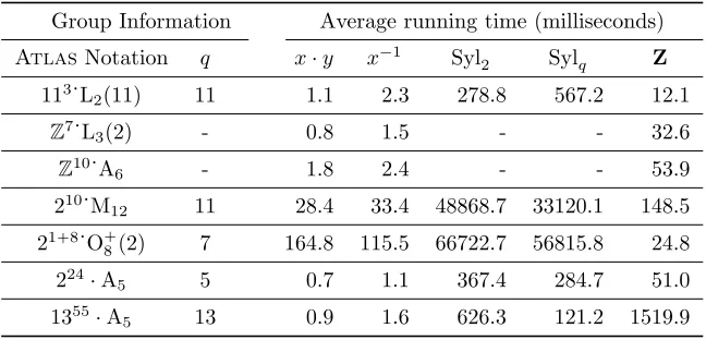
6. Implementation and Examples
The suite of algorithms described in the paper have been implemented using the Magma Computational Algebra System. Table 1 gives running times for a sample of test groups.
The format of Table 1 is as follows. The first column gives the Atlas
notation of the group. The largest primeqdividing the order of the group (when the group is finite) is given in the second column. The remaining columns give the running times (in milliseconds, averaged over 100 runs, randomised where applicable) to perform the indicated computation.
The first four examples in Table 1 are extensions of modules by their groups; these groups are constructed with the help of the natively implemented coho-mology functions in Magma. The last two examples in Table 1 are quotients of finitely presented groups, each of which map ontoA5.
The first entry of Table 1 is a non-split extension of the irreducible module
pZ{11Zq3by PSLp2,11q. It has relatively small order (878460) and has minimal degree of permutation representation 132.
The fourth entry of Table 1 is a non-split extension of the irreducible module
pZ{2Zq10byM12. It has order 216¨33¨5¨11 and minimal degree of permutation representation 264.
The fifth entry of Table 1 is a non-split extension of an extra special group of order 29 by O`8p2q. It has order 221¨35¨52¨7, and the authors have obtained a permutation representation of this group having degree 34560.
The last two entries of Table 1 are finitely presented groups, each of which map ontoA5. The penultimate entry is a quotient of the Heineken group,
H “ xa, b, c| ra,ra, bss “c,rb,rb, css “a,rc,rc, ass “by.
The quotient has order 226
¨3¨5, and the authors conjecture that the minimal degree of a permutation representation of this group is 138240.
The final entry is a quotient of the group having presentation
xa, b, c|a2, b3,pabq5, abcb´1ac´1b´1c´1bc´1
y.
The quotient has order 22¨3¨5¨1355. The minimal degree of a permutation representation of this group is unknown, but the authors believe that it is too large to be computationally useful.
Benchmark running times are not available, as there is no existing standard method in Magma to perform most of the computations listed, and, in the case of the last two groups of Table 1, it is not possible to natively construct the extension.
[image:21.612.144.468.471.627.2]The tests were performed on a system with the following specifications: 16GB memory, 2.90GHz quad-core processor, Linux kernel version 3.16.0, Magma V2.21-7.
Table 1: Sample running times
Group Information Average running time (milliseconds)
AtlasNotation q x¨y x´1 Syl
2 Sylq Z
113¨L
2p11q 11 1.1 2.3 278.8 567.2 12.1
Z7¨L3p2q - 0.8 1.5 - - 32.6
Z10¨A6 - 1.8 2.4 - - 53.9
210¨M12 11 28.4 33.4 48868.7 33120.1 148.5
21`8¨O`
8p2q 7 164.8 115.5 66722.7 56815.8 24.8
224¨A5 5 0.7 1.1 367.4 284.7 51.0
1355
7. Conclusion
The running times of Table 1 are encouraging. Since the computations described involve large numbers of executions of individual group operations, such as mulitplication and conjugation, it is possible that the Magma interpreter is causing a significant overhead, and that running times could be significantly improved by a native implementation.
One expects that, after optimised implementation, the data structure and algorithms described in this paper would become a suitable option for computa-tion with polycyclic-by-finite groups for which there is no available permutacomputa-tion or matrix representation, but whose finite quotient is relatively small and easily represented as a permutation group.
8. Acknowledgements
The authors would like to thank Colva Roney-Dougal for her helpful sug-gestions. We would also like to recognise David Howden whose work on au-tomorphism groups has helped in the construction of some of the motivating examples.
9. Bibliography
Baumslag, G., Cannonito, F. B., Robinson, D. J. S., Segal, D., 1991. The Al-gorithmic Theory of Polycyclic-by-Finite Groups. Journal of Algebra 142, 118–149.
Dixon, J. D., 1982. Exact solution of linear equations using p-adic expansion. Numerische Mathematik 40, 137–141.
Eick, B., 2001. Algorithms for Polycyclic Groups. Habilitationsschrift, Univer-sit¨at Kassel.
Glasby, S. P., Slattery, M. C., 1990. Computing intersections and normalizers in soluble groups. J. Symbolic Comput. 9, 637–51.
Haramoto, H., Matsumoto, M., 2009. Ap-adic algorithm for computing the in-verse of integer matrices. Journal of Computational and Applied Mathematics 225, 320–322.
Holt, D. F., Eick, B., O’Brien, E. A., 2005. Handbook of Computational Group Theory. Discrete Mathematics and its Applications. Chapman & Hall/CRC.
Hulpke, A., 2013. Computing conjugacy classes of elements in matrix groups. Journal of Algebra 387, 268–286.
Mecky, M., Neub¨user, J., 1989. Some remarks on the computation of conjugacy classes of soluble groups. Bull. Australian Math. Soc. 40, 281–92.
Seress, ´A., 2003. Permutation Group Algorithms. Vol. 152 of Cambridge Tracts in Mathematics. Cambridge University Press.
Sims, C. C., 1970. Computational methods in the study of permutation groups. In: Leech, J. (Ed.), Computational Problems in Abstract Algebra. Pergamon Press, Oxford, pp. 169–183.
Sims, C. C., 1971. Computation with permutation groups. In: Proc. Second Symposium on Symbolic and Algebraic Manipulation. ACM Press, New York, pp. 23–28.