warwick.ac.uk/lib-publications
A Thesis Submitted for the Degree of PhD at the University of Warwick
Permanent WRAP URL:
http://wrap.warwick.ac.uk/107784
Copyright and reuse:
This thesis is made available online and is protected by original copyright.
Please scroll down to view the document itself.
Please refer to the repository record for this item for information to help you to cite it.
Our policy information is available from the repository home page.
U N
IV
ER
SITAS WARWICEN SIS
Energy-Aware Performance Engineering in
High Performance Computing
by
Stephen Ian Roberts
A thesis submitted to The University of Warwick
in partial fulfilment of the requirements
for admission to the degree of
Doctor of Philosophy
Department of Computer Science
The University of Warwick
Advances in processor design have delivered performance improvements for
decades. As physical limits are reached, however, refinements to the same basic
technologies are beginning to yield diminishing returns. Unsustainable increases
in energy consumption are forcing hardware manufacturers to prioritise energy
efficiency in their designs. Research suggests that software modifications will be
needed to exploit the resulting improvements in current and future hardware.
New tools are required to capitalise on this new class of optimisation.
This thesis investigates the field of energy-aware performance engineering.
It begins by examining the current state of the art, which is characterised by
ad-hoc techniques and a lack of standardised metrics. Work in this thesis addresses
these deficiencies and lays stable foundations for others to build on.
The first contribution made includes a set of criteria which define the
proper-ties that energy-aware optimisation metrics should exhibit. These criteria show
that current metrics cannot meaningfully assess the utility of code or correctly
guide its optimisation. New metrics are proposed to address these issues, and
theoretical and empirical proofs of their advantages are given.
This thesis then presents the Power Optimised Software Envelope (POSE)
model, which allows developers to assess whether power optimisation is worth
pursuing for their applications. POSE is used to study the optimisation
charac-teristics of codes from the Mantevo mini-application suite running on a
Haswell-based cluster. The results obtained show that of these codes TeaLeaf has the
most scope for power optimisation while PathFinder has the least.
Finally, POSE modelling techniques are extended to evaluate the
system-wide scope for energy-aware performance optimisation. System Summary POSE
allows developers to assess the scope a system has for energy-aware software
I am indebted to many people for their support, guidance and friendship during
my time at the University of Warwick. It gives me great pleasure to acknowledge
a small number of them here.
First and foremost I am grateful to my supervisor, Prof. Stephen Jarvis,
who gave me the opportunity to undertake this research. He has remained a
constant source of advice and encouragement throughout my Ph. D.
I am also extremely grateful to Dr. Suhaib Fahmy for his help and guidance.
Suhaib has always gone the extra mile to help, and my research into optimisation
metrics in particular would not have been possible without his input.
I would like to thank my lab partners and colleagues in the Department of
Computer Science, including Dr. Steven Wright, Dr. Philip Taylor, Dr. Richard
Bunt, Dr. Arshad Jhumka, Dr. Adam Chester, Tim Law, Huanzhou Zhu and
Andrew Owenson. Their perspectives and insights have proven invaluable.
I also wish to thank the Center of Information Services and High Performance
Computing (ZIH) at TU Dresden. Much of this work has benefited from access
to their power instrumented supercomputing hardware. A special vote of thanks
is owed to Thomas Ilsche for his patience and generosity.
Returning to academia from industry was a leap of faith which would not
have been possible without the support of past colleagues. Special thanks in
this regard go to Dr. Enrico Scalavino for our many discussions on the subject.
Thanks also go to Zheng Huang, Nic Quilici and Amaury Chamayou.
Finally, I would like to thank my friends and family for their support and
kindness. Mum, Dad, my cousins David, Dereck and William, my sister Annie
and aunt Ann, and also to my uncle Grahame, who sadly left us before this
This thesis is submitted to the University of Warwick in support of my
appli-cation for the degree of Doctor of Philosophy. It has been composed by myself
and has not been submitted in any previous application for any degree.
Parts of this thesis have been published by the author:
[104] S. I. Roberts, S. A. Wright, D. Lecomber, C. January, J. Byrd, X. Or´o, and
S. A. Jarvis. POSE: A Mathematical and Visual Modelling Tool to Guide
Energy Aware Code Optimisation. InProceedings of the 6th International
Green and Sustainable Computing Conference (IGSC ’15), December 2015
[105] S. I. Roberts, S. A. Wright, S. A. Fahmy, and S. A. Jarvis. Metrics for
Energy-Aware Software Optimisation.Lecture Notes in Computer Science
(LNCS), 10266:413–430, June 2017
[103] S. I. Roberts, S. A. Wright, S. A. Fahmy, and S. A. Jarvis. The
Power-Optimised Software Envelope. ACM Transactions on Architecture and
The research presented in this thesis was made possible in part by the support
of the following benefactors:
• Technology Strategy Board project number 131197 (Energy-Efficiency Tools
ADP Area Delay Product . . . 50
ALU Arithmetic Logic Unit . . . 38
ATX Advanced Technology eXtended . . . 12
CISC Complex Instruction Set Computing . . . 16
CMOS Complimentary Metal Oxide Semiconductor . . . 34
CPU Central Processing Unit . . . 1
CRCW Concurrent Read Concurrent Write . . . 29
CREW Concurrent Read Exclusive Write . . . 29
DAG Directed Acyclic Graph . . . 24
DMM Distributed Memory Machine . . . 8
DVFS Dynamic Voltage and Frequency Scaling . . . 33
EDD Energy Delay Distance . . . 60
EDP Energy Delay Product . . . 48
EDS Energy Delay Sum . . . 60
ENIAC Electronic Numerical Integrator and Computer . . . 35
ERCW Exclusive Read Concurrent Write . . . 29
EREW Exclusive Read Exclusive Write. . . .29
FLOPS Floating Point Operations per Second . . . 17
FoM Figure of Merit . . . 15
FPE Feasible Performance Envelope . . . 71
FPGA Field-Programmable Gate Array . . . 2
IBS Instruction Based Sampling . . . 20
IC Integrated Circuit . . . 3
ICC Intel C++ Compiler . . . 66
ILP Instruction Level Parallelism . . . 26
IPS Instructions Per Second . . . 16
ITUE Information Technology Power Usage Effectiveness . . . 17
MIMD Multiple Instruction Multiple Data . . . 8
MISD Multiple Instruction Single Data . . . 8
MOO Multi-Objective Optimisation. . . .15
MSR Model Specific Register . . . 13
MTTF Mean Time To Failure . . . 4
NASA National Aeronautics and Space Administration . . . 45
NUMA Non-Uniform Memory Access . . . 9
PDP Power Delay Product . . . 50
PEBS Precise Event-Based Sampling . . . 20
POSE Power Optimised Software Envelope . . . 5
PRAM Parallel Random Access Machine . . . 28
PUE Power Usage Effectiveness . . . 17
RAPL Running Average Power Limit . . . 13
RISC Reduced Instruction Set Computing . . . 16
SIMD Single Instruction Multiple Data . . . 3
SISD Single Instruction Single Data . . . 8
STFC Science and Technology Facilities Council. . . .118
TCO Total Cost of Ownership . . . 4
TDP Thermal Design Power . . . 42
Abstract i
Dedication ii
Acknowledgements iii
Declarations iv
Sponsorship and Grants v
Abbreviations vi
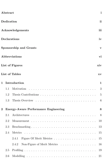
List of Figures xiv
List of Tables xv
1 Introduction 1
1.1 Motivation . . . 3
1.2 Thesis Contributions . . . 5
1.3 Thesis Overview . . . 6
2 Energy-Aware Performance Engineering 8 2.1 Architectures . . . 8
2.2 Measurement . . . 10
2.3 Benchmarking . . . 13
2.4 Metrics . . . 15
2.4.1 Figure Of Merit Metrics . . . 15
2.4.2 Non-Figure of Merit Metrics . . . 16
2.5 Profiling . . . 19
[image:11.595.121.470.169.711.2]2.6.3 Simulation . . . 30
2.7 Optimisation . . . 31
2.7.1 Energy-Aware Optimisation . . . 32
2.8 Summary . . . 33
3 Energy Efficiency in Computer Systems 34 3.1 Fabrication Technologies . . . 34
3.2 CMOS Digital Logic . . . 37
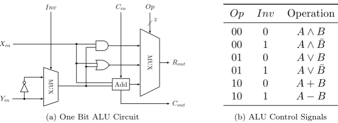
3.2.1 Arithmetic Logic Unit Design . . . 38
3.3 CMOS Power Draw . . . 40
3.4 Architectural Energy Efficiency Features . . . 42
3.4.1 Multi-core Processors . . . 43
3.4.2 Clock Gating . . . 43
3.4.3 Dynamic Voltage and Frequency Scaling . . . 44
3.4.4 Heterogeneous Computing . . . 44
3.5 Energy Efficiency Trends . . . 45
3.6 Summary . . . 47
4 Metrics for Energy-Aware Software Optimisation 48 4.1 Delay Product Metrics . . . 48
4.2 Software Optimisation Metrics . . . 51
4.3 Etn Evaluation . . . . 54
4.3.1 Justification ofEtn. . . . 59
4.4 Proposed Metrics . . . 60
4.4.1 Proposed Metric 1: Energy Delay Sum . . . 60
4.4.2 Proposed Metric 2: Energy Delay Distance . . . 63
4.5 Case Study . . . 65
5.1.1 Feasible Performance Envelope . . . 71
5.1.2 Optimisation Bound . . . 72
5.1.3 Contribution Bound . . . 74
5.1.4 Optimisation Limit . . . 77
5.2 POSE Insights . . . 78
5.3 POSE Models for Novel Metrics . . . 80
5.3.1 Energy Delay Sum POSE . . . 82
5.3.2 Energy Delay Distance POSE . . . 85
5.4 POSE Investigation . . . 90
5.4.1 Feasible Performance Envelope . . . 91
5.4.2 POSE Models for Code Optimisation . . . 93
5.4.3 POSE Models for Frequency Scaling . . . 95
5.4.4 POSE Models for Distributed Codes . . . 98
5.5 Summary . . . 99
6 System Summary POSE 101 6.1 System Summary POSE Derivation . . . 101
6.2 System Summary POSE for Novel Metrics . . . 105
6.2.1 Energy Delay Sum System Summary POSE . . . 106
6.2.2 Energy Delay Distance System Summary POSE . . . 107
6.3 System Summary POSE Investigation . . . 108
6.4 Optimisation Study . . . 110
6.5 Summary . . . 113
7 Conclusions and Future Work 116 7.1 Thesis Limitations . . . 118
7.2 Future Work . . . 119
Appendices 138
A POSE Model Summary for Different Metrics 138
A.1 Etn POSE . . . 138
A.2 Energy Delay Sum POSE . . . 138
A.3 Energy Delay Distance POSE . . . 139
B Mantevo Suite POSE Models 140
2.1 Crossbar Network Topology . . . 9
2.2 PowerMon Current Sense Resistor Circuit . . . 11
2.3 Amdahl’s Law Speed-up Limits . . . 23
2.4 Amdahl’s Law Efficiency Limits . . . 23
2.5 Work, Span and Maximum Cut . . . 25
2.6 Example Roofline Model . . . 26
2.7 Powerline Model . . . 27
2.8 PRAM Abstract Machine Model . . . 29
3.1 Power Density Trends, based on data from [22] . . . 36
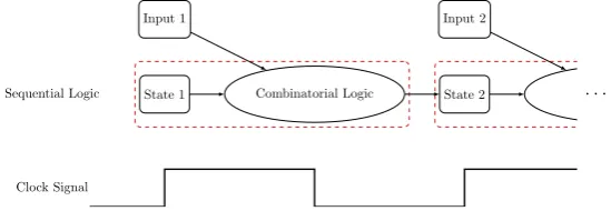
3.2 Synchronous Sequential Logic . . . 37
3.3 One Bit ALU Schematic . . . 38
3.4 Combinatorial ALU . . . 39
3.5 Sequential ALU . . . 40
4.1 Design Trade-Off Constraint Diagram . . . 49
4.2 Metric Optimisation Regions . . . 52
4.3 Etn Metric Fitness Landscapes . . . . 53
4.4 Etn Optimisation Instability . . . . 57
4.5 Power-Limited Isometric Lines . . . 60
4.6 Proposed Metrics Fitness Landscapes . . . 61
4.7 Energy Delay Distance Instability . . . 65
5.1 Et2 Power Optimised Software Envelope . . . . 72
5.2 Et2 Power Optimised Software Envelope Regions . . . . 79
5.3 Etn POSE Model Tunability . . . 81
5.7 Et2 POSE for P-State Optimisation of TeaLeaf and MiniMD . . 97
5.8 Et2 POSE for Multi-Node Runs of TeaLeaf and MiniMD . . . . 98
6.1 Et2 System Summary POSE Intuition . . . 102
6.2 Optimisation Limits . . . 110
6.3 1D Trapezoidal Decomposition . . . 112
3.1 Pleiades CPU Upgrades . . . 46
4.1 Single Node Code Costs . . . 67
4.2 MiniMD Multi-Node Costs . . . 67
5.1 Single Node Feasible Performance Envelope Parameters . . . 93
5.2 Code Metrics forS= 2.5 GHz,C= 24 . . . 94
5.3 Et2 POSE Model Summaries . . . . 95
5.4 MiniMD POSE Models for Novel Metrics . . . 95
6.1 Optimisation Impact . . . 113
B.1 Et2 POSE Model Summaries for Remaining Codes . . . 141
B.2 EDS POSE Model Summaries (α= 1, β= 900) . . . 142
B.3 EDD POSE Model Summaries (α= 1, β= 519.615) . . . 143
Introduction
Scientific computing and numerical simulation have become indispensable tools
in many areas of science and engineering. Simulations allow scientists to test
their theories in domains where physical experimentation would be prohibitively
costly, impractical, or dangerous. As a result, computational methods have
joined theory and experiment as central pillars of scientific investigation [57].
Maximising performance is paramount in scientific computing. Higher
per-formance means more calculations can be carried out, allowing scientists to
increase the size, complexity or resolution of their simulations. This demand
for performance has led to the development ofsupercomputers, large machines
orders of magnitude more powerful than desktop computers.
Supercomputers are typically constructed by linking many smaller nodes
together to form a cluster. Specialist tools and programming models are then
used to write software that can be run on several nodes in parallel. These nodes
communicate over an interconnect network, collaborating to run simulations
and produce results faster than a single node could manage in isolation.
The field of High Performance Computing (HPC) exists to improve the
per-formance of supercomputers and the software which they run. HPC covers a
broad spectrum of disciplines. At one extreme, domain experts write high-level
simulation software to model phenomena of interest. At the other, hardware
engineers design the processors and other components that make up
super-computers. Performance engineering bridges the gap between these extremes,
seeking ways to optimise software to make better use of the available hardware.
Moore’s law states that transistor density doubles every 18-24 months [93].
performance for decades. Dennard scaling, which states that the power use of
transistors is proportional to their size [28], kept energy consumption in check as
increasing numbers of transistors were packed into CPUs. Together, these laws
led to a period known as the “Free Lunch”, when rising clock speeds delivered
regular performance increases with no additional power cost.
Dennard scaling ended around 2006 [52], and Moore’s law is also
show-ing signs of failure [116]. Refinements to the same underlyshow-ing technologies are
yielding diminishing returns, and the “Free Lunch” is now over [115]. Energy
consumption is rapidly becoming a limiting factor for continued progress in
scientific computing as a result [109].
The end of Dennard scaling has forced hardware engineers to prioritise
en-ergy efficiency in their designs. This has lead to both modifications in existing
platforms as well as the development of new HPC technologies. Some of these
novel technologies are pre-existing products which have been repurposed for
scientific computing. Examples of this kind include Field-Programmable Gate
Arrays (FPGAs) [29], general purpose Graphics Processing Units (GPUs) [46]
and Intel’s Xeon Phi coprocessors [21]. Others, like NEC’s Aurora Vector
En-gine, were designed specifically for the HPC market.
Performance engineers are also feeling the effects of this drive towards
en-ergy efficiency. One obvious example is the emergence of new programming
models like OpenACC, OpenCL and CUDA which allow developers to target
the novel energy-efficient accelerator technologies listed above. More subtly,
re-search suggests that targeted modifications to existing software will be required
to fully exploit the energy efficiency improvements in modern hardware [111].
New energy-aware performance engineering techniques are being developed to
identify and capitalise on this new class of optimisation.
This work investigates how conventional performance engineering techniques
can be adapted to support energy-aware software optimisation. It highlights
challenges which must be overcome before this new class of optimisation can be
be expected as a result of energy-aware optimisation.
1.1
Motivation
Moore’s law was first proposed in 1965 and quickly became a self-fulfilling
prophecy as hardware manufacturers were forced to keep up with it or face
being overtaken by their competition. This resulted in a doubling of transistor
density every 18-24 months, fuelled by advances in Integrated Circuit (IC)
fab-rication, circuit design and processor architectures. Moore’s Law has driven the
development of computer hardware in this way for decades.
The area occupied by individual transistors halves with every doubling of
transistor density. Power density (i.e. the rate of power consumption per unit
area) remained constant under Dennard scaling, so the power consumed by
each transistor was also halved. This in turn led to faster clock speeds as the
maximum switching frequency of a transistor is inversely proportional to its
peak power consumption [61].
Clock speeds increased exponentially with each new generation of
proces-sors while Dennard scaling persisted. The “Free Lunch” period resulted from
this link between transistor density and processor speed. The link was broken
when Dennard scaling ended, causing clock speeds to stagnate even as
transis-tor densities continued to rise. Hardware designers now rely on architectural
changes such as vectorisation, superscalar architectures and multiple cores to
deliver performance improvements [95].
Higher clock speeds deliver performance improvements without developer
input, hence the term “Free Lunch”. Conversely, software modifications are
required to take advantage of novel hardware features. New instructions are
needed for Single Instruction Multiple Data (SIMD) vectorisation, for example,
and applications must be parallelised to run on multiple cores. Although
com-pilers can perform some of this work, performance engineers typically have to
Processor power density has been rising since the end of Dennard scaling.
This trend has been partially offset by one-off advances in fabrication processes
and the use of exotic materials in transistors. Such advances only provide
tem-porary reprieve, however, and the overall trend is expected to continue [37].
Rising power density poses a number of challenges to the field of HPC. First,
energy costs are soaring as increased per-processor power draw is compounded
by the growing number of processors used in modern supercomputers. These
costs already represent a large share of the Total Cost of Ownership (TCO) for
supercomputing systems and are expected to rise still further [108].
Secondly, higher power densities lead to increased operating temperatures,
which can cause problems with hardware reliability [112]. At present, around
20 % of the available compute time on large-scale supercomputers is lost due to
hardware failures [34]. This trend is also exacerbated by high processor counts,
as shortening the Mean Time To Failure (MTTF) of individual processors has
a cumulative effect on the MTTF of machines as a whole.
Finally, power density cannot continue to grow indefinitely. There are limits
to how much power can be delivered to processors and how quickly the resulting
heat can be removed. If performance improvements cannot be decoupled from
increasing power density then these too will come to an end.
Hardware designers are responding to these challenges by prioritising energy
efficiency in their processor designs. Improving energy efficiency through
archi-tectural changes closely parallels the way in which performance improvements
are currently delivered. The expected outcome is also the same; code changes
will be needed in order to maximise the benefits of energy efficient hardware
features. Energy-aware performance engineering techniques will therefore be
required as power becomes a first-class constraint in HPC.
The US Department of Energy has identified energy efficiency as a primary
constraint for exascale systems [109]. New performance engineering approaches
will be required soon if the current rate of progress in HPC is to be maintained.
experi-ence adapting software to maximise performance on new hardware. This thesis
aims to show how these existing tools and techniques can be updated to consider
energy as well as runtime.
Energy-aware performance optimisation is still in its infancy, characterised
by ad-hoc techniques and a lack of standardised metrics. This thesis contributes
a set of metrics which are shown to be more suitable for use in guiding
energy-aware optimisation than current alternatives. It also presents a pair of related
approaches for identifying the potential for energy-aware optimisation, one for
individual codes and the other for entire systems.
The techniques described in this thesis are notable for their generality. They
are not platform or application specific and impose very few prerequisites on
their use. Despite this, they are able to provide immediate, actionable insights
to performance engineers and software developers.
1.2
Thesis Contributions
This thesis makes the following specific contributions:
• New metrics are developed to guide and assess energy-aware code
optimi-sations. In the absence of better alternatives, performance engineers have
turned to metrics developed by the hardware community. These hardware
metrics are ill-suited to software optimisation, and the lack of
standard-isation makes comparing results between studies impossible. This thesis
seeks to address both of these shortcomings by introducing a common set
of metrics along with rigorous justification of their utility.
• This thesis presents the Power Optimised Software Envelope (POSE), a
model which helps performance engineers to determine whether energy
or runtime optimisation will provide the greatest benefits for their code.
The POSE model is platform agnostic, meaning it can be applied to any
• The POSE model is extended to provide a model for system-wide power
optimisation characteristics. System Summary POSE is able to derive
upper limits for the benefit of energy-aware software optimisation on a
given system. This allows developers to determine how amenable a system
is to energy optimisation and hence whether it may be worth pursuing on
their chosen platform in general, independent of any specific codes.
1.3
Thesis Overview
The remainder of this thesis is structured as follows:
Chapter 2provides an account of core concepts, techniques and terminology
employed in the field of HPC. Contemporary performance engineering tools and
practices are described, and their suitability for energy-aware software
optimi-sation is assessed. This chapter includes an overview of relevant performance
engineering literature.
Chapter 3details the evolution of parallel computing hardware with an
empha-sis on energy efficiency. The problems which motivate this work arise because
hardware development is failing to maintain past trends in power consumption.
This chapter provides a generalised model of hardware power consumption, and
introduces features found in modern processors designed to minimise it. A key
aim of this chapter is to highlight various ways in which performance engineers
can influence energy efficiency.
Chapter 4 examines the metrics currently used to guide energy-aware
per-formance optimisation. A good metric should provide meaningful values for a
single experiment, allow fair comparison between experiments, and drive
opti-misation in a sensible direction. This chapter shows that established metrics are
Chapter 4 concludes with theoretical and empirical proofs of the advantages of
these new metrics over established alternatives.
Chapter 5introduces the POSE model. POSE serves as a preliminary “first
cut” modelling technique intended to guide energy-aware optimisation efforts.
This model presents an asymptotic analysis of the scope a code has for
optim-sation in both the power and runtime domains. By identifying the limits of
each approach, POSE allows performance engineers to make informed decisions
about where to focus their efforts in order to achieve the best results.
Chapter 6 builds on previous chapters by extending POSE to model
system-wide optimisation criteria. Conventional POSE models use the runtime and
energy costs of a code to calculate the scope that code has for power and
run-time optimisation on a given system. Conversely, System Summary POSE is a
meta-heuristic which determines the range of results POSE models could
pro-duce for a given system. This bound-of-bounds analysis places limits on the
system-wide scope for power optimisation independent of any specific codes.
Chapter 7 concludes this work with a summary of results and contributions
made, and discusses their implications for performance engineers. It also
consid-ers the future direction of energy-aware performance engineering and provides
Energy-Aware Performance Engineering
This chapter introduces core concepts, techniques and terminology in the field
of High Performance Computing (HPC). These topics are divided into seven
areas, namely: Architectures, Measurement, Metrics, Benchmarking, Profiling,
Modelling, and finally Optimisation. Energy-aware performance engineering
re-quires new developments to be made in each of these areas. Recent developments
are discussed, and areas where progress is lacking are highlighted.
2.1
Architectures
In simplest terms, supercomputers are nothing more than large collections of
processing elements working together to solve complex problems [7]. This
de-scription is general enough to encompass the wide range of architectures which
have been used to construct HPC systems over the years.
Flynn’s taxonomy classifies computer architectures based on how many
in-structions and data items they can handle concurrently [39]. In this taxonomy,
Single Instruction Single Data (SISD) architectures are those which do not
ex-hibit any kind of parallelism. Single Instruction Multiple Data (SIMD)
archi-tectures execute their instructions sequentially, but each instruction operates
on multiple data elements in parallel. Multiple Instruction Single Data (MISD)
architectures execute multiple instructions on the same piece of data in
paral-lel. Finally, Multiple Instruction Multiple Data (MIMD) architectures execute
multiple instructions on their own independent data in parallel.
Modern supercomputers predominantly use MIMD architectures [102]. These
systems can be divided into Distributed Memory Machines (DMMs) and Shared
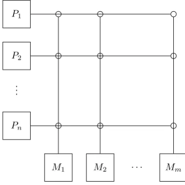
P1
P2
.. .
Pn
[image:26.595.199.389.129.319.2]M1 M2 · · · Mm
Figure 2.1: Crossbar Network Topology
DMMs consist of multiple compute nodes connected to each other through a
shared interconnect. These nodes are independent units with their own
proces-sors, memory and peripherals. Data held by a node in local memory is private
and cannot be accessed directly by other nodes. Explicit message passing
pro-tocols are used to allow groups of nodes to collaborate and share data.
SMMs consist of multiple processors all connected to a large pool of shared
memory made up of many discrete memory modules. A common address space
allows processors to access shared data transparently, regardless of its physical
location. SMMs are further sub-divided into Symmetric Multiprocessing (SMP)
and Non-Uniform Memory Access (NUMA) machines.
Processors in SMP machines have fast access to all areas of shared memory.
Conceptually, allM×N pairs of memory modules and processors are connected
by a flat network topology like the crossbar network shown in Figure 2.1. The
scalability of SMP machines is limited by resource contention and the need for
expensive, densely connected interconnects.
NUMA systems improve scalability by giving processors faster access to their
own local memory. Other machines can still access this memory, however they
exhibit data locality as only remote memory accesses travel over the network.
Flynn’s taxonomy also applies at the level of individual processors.
Mod-ern CPUs support both SIMD and MIMD operations through vector
instruc-tions and multiple cores respectively. There are no MISD implementainstruc-tions
in widespread use for HPC, however some Field-Programmable Gate Array
(FPGA) design patterns come close [5].
An ongoing trend in HPC is the shift towardsheterogeneouscomputing [77].
In addition to conventional CPUs, heterogeneous systems also incorporate
spe-cialised compute devices calledacceleratorsorcoprocessors to handle particular
tasks. Devices like Graphics Processing Units (GPUs), FPGAs and Intel’s Xeon
Phi coprocessors can be used to speed up execution of computationally intensive
codes while also reducing system energy consumption [35].
2.2
Measurement
Accurate measurement is fundamental to performance engineering. Processors
incorporate built-in clocks to maintain synchronisation and schedule interrupts.
Engineers can use these clocks to measure the runtime performance of their code.
Energy monitoring capabilities are also appearing in new processor designs.
Energy is the integral of power over time, orE = ¯P t. Energy consumption
cannot be measured directly as a consequence, and must instead be calculated
from measurements of power draw and time.
Various methods have been used to measure power draw in HPC systems,
both at system and component levels. One approach uses thermal cameras
to measure the temperature of different components and hence estimate their
power draw. This works because the energy used by computers is converted
to waste heat in accordance with the first law of thermodynamics.
Mesa-Martinez et al. used thermal cameras and custom heat sinks to measure Central
Processing Unit (CPU) power consumption [92], while Hackenberg et al.
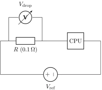
R(0.1 Ω)
+ −
Vref
V
Vdrop
[image:28.595.211.384.126.278.2]CPU
Figure 2.2: PowerMon Current Sense Resistor Circuit
The main advantage of this approach is its high spatial resolution; thermal
im-agery is able to show how power draw varies between components, and even
across different areas of the same component. One disadvantage is poor
tempo-ral resolution; materials absorb heat and release it over time, meaning thermal
emissions correspond to a moving average of power consumption. Another
dis-advantage is the requirement for expensive cameras and custom heat sinks,
which makes this approach prohibitively costly when applied at scale.
Higher temporal resolution can be obtained at relatively low cost by
in-strumenting computing platforms with dedicated power sensors. Bedard et al.
developed PowerMon, a scheme for measuring component-level power draw in
commodity systems [10]. PowerMon works by measuring the voltage dropVdrop
across resistors placed inline between the power supply and other system
com-ponents. These resistors are calibrated to ensure they provide a particular
resistanceR(0.1 Ω is typical). Figure 2.2 shows a simplified circuit diagram for
their apparatus.
I= V
R (2.1)
PowerMon uses Ohm’s law as stated in Equation 2.1 to calculate current flow
flow in this manner are referred to as ‘sense’ or ‘shunt’ resistors. The same
amount of current flows through both the sense resistor and the component being
measured because current is conserved throughout series circuits. Furthermore,
supply voltageVreftakes on a known value depending on the type of component
being powered. The Advanced Technology eXtended (ATX) standard mandates
power supply output voltages of 12 V, 5 V, 3.3 V and −12 V, for example [23].
Component power draw can then be calculated as the product ofI andVrefas
per Equation 2.2.
P =IV (2.2)
Sense resistors have three major drawbacks when used in HPC systems. First,
some energy is lost as heat within the resistor, increasing overall power draw.
Secondly, their resistance varies with temperature, limiting accuracy and
in-troducing non-linearities in their results. Finally, they require direct electrical
connections to the power supply and the component being measured. Any
short-circuits or other manufacturing defects could easily damage sensitive hardware.
An alternative approach to power measurement relies on the magnetic fields
induced when current flows through a wire. Ampere’s law for straight
con-ductors, given by Equation 2.3, states that the magnetic field strength |B~| at
distancerfrom the wire is proportional to the original currentI. The constant
µcorresponds to the magnetic permiability of air.
|B~|= µ I
2πr (2.3)
Hall effect sensors measure magnetic field strength, and can therefore be used to
determine current flow while remaining electrically isolated from the conductor.
Laros et al. developed PowerInsight, a production quality power monitoring
platform which uses Hall effect sensors rather than sense resistors to improve
accuracy and reliability [81]. Equation 2.2 is again used to calculate power
Hackenberg et al. instrumented a large HPC cluster called Taurus with
com-mercial power sensors which exploit the Hall effect. The resulting High Density
Energy Efficiency Monitoring (HDEEM) infrastructure can be used to measure
component-level power and energy consumption across large numbers of nodes
at high sample rates [51].
Intel introduced Running Average Power Limit (RAPL) to support
power-aware frequency scaling in their Sandy Bridge Processors [27]. As a side
ef-fect, performance engineers gained access to an interface capable of reporting
CPU power consumption. RAPL exposes a number of Model Specific
Regis-ters (MSRs) which can be read by user code to determine the rate of power
draw. Early versions of RAPL were model based, but more recent processors
incorporate dedicated power sensors.
Other manufacturers have also added power measurement capabilities to
their hardware. AMD added a scheme similar to RAPL with equivalent
func-tionality starting with their Bulldozer CPUs [1]. Similar schemes also exist for
GPUs [18] and Xeon Phi [82] hardware.
HPC Vendors and system integrators are also beginning to include power
monitoring capabilities in their products. Cray’s XC line of supercomputers
expose energy measurements through systems [55]. Similarly, IBM servers
in-corporate current measuring hardware based on sense resistors which can be
read using their Amester tool [16].
2.3
Benchmarking
Modern processors include hardware designed to accelerate specific operations.
Vendors quote peak performance figures which assume that all these hardware
features can be kept fully occupied. In practice, applications only perform a
subset of the relevant operations, and memory bandwidth limits often prevent
those features which are used from achieving maximum throughput.
Performance benchmarks serve a dual purpose. First, benchmarks can be used
to measure and compare the performance realistically achievable by different
machines and architectures. Secondly, benchmarks serve as good platforms to
investigate the effects of different optimisations in a controlled manner.
Micro-benchmarksare simple programs designed to target specific aspects of
system performance. Linpack is a well known micro-benchmark which measures
a system’s capacity for sustained floating point throughput [30]. Linpack results
form the basis of the Top500 and Green500 supercomputer rankings [38]. Other
micro-benchmarks include STREAM [90], which measures memory bandwidth;
SKaMPI, which measures network performance [4]; and IOR, which measures
file system performance [110].
Application benchmarks are larger programs which test how well systems
handle complex applications. They are often built from simplified versions of
production applications in order to ensure realistic workloads. The Mantevo
project is a suite of application benchmarks developed at Sandia National
Lab-oratories [56] and used extensively throughout this thesis.
Existing benchmarks can be repurposed for power and energy studies [72],
and dedicated power benchmarks have also started to emerge. One example is
FIRESTARTER [50], a micro-benchmark specifically designed to trigger
near-peak power consumption across a range of x86 64 CPUs and NVIDIA GPUs.
It contains hand optimised assembly routines which raise processor activity
above the level attainable with high level languages. A small assembly
micro-benchmark designed to minimise power consumption while keeping CPUs active
is also described in this thesis.
SPECpower is a commercial benchmarking suite which provides an
applica-tion benchmark called “SPECPower ssj2008” along with a framework for
mea-suring application energy efficiency and performance [79]. The SPECpower
benchmark is a Java program which simulates a transactional workflow running
under varying amounts of load. It is designed to mimic the behaviour of common
which must handle bursts in utilization. SPECpower measures performance at
11 different target loads, starting at 100% utilization and reducing this in steps
of 10% until it reaches idle.
2.4
Metrics
Performance engineers use metrics to assess the performance of HPC hardware
and software. Individual metrics capture particular properties of a system under
investigation. Some of these properties can be measured directly, while others
must be derived from multiple observations.
Metrics enable meaningful comparison between different platforms and can
be used to quantify the effects of code changes. They can be divided into two
categories depending on the types of comparison they allow; namely Figure of
Merit (FoM) and Non-FoM metrics.
2.4.1
Figure Of Merit Metrics
Some metrics act as utility functions which measure the cost of running different
programs. These FoM metrics can be used to rank different implementations of
the same algorithm in order to identify valid optimisations [53]. Runtime and
energy consumption are both examples of FoM metrics.
Until recently, runtime optimisation was ubiquitous in HPC while energy
optimisation has been confined to domains like embedded systems and mobile
robotics. Although energy consumption is becoming a constraint for scientific
computing, minimising runtime is still an important optimisation objective.
Optimising software according to multiple properties simultaneously is known
as Multi-Objective Optimisation (MOO). MOO requires FoM metrics that
strike the right balance between the potentially conflicting requirements
im-posed by different optimisation objectives.
Gonzalez et al. proposed Energy Delay Product, a FoM metric which
generalised this into the Etn family of FoM metrics, with parametersE andt
corresponding to energy and time [88]. They argue thatEt2 provides the best
balance for microprocessor design. Srinivasan et al. reached the same conclusion,
although for slightly different reasons [113].
Many authors have adopted these metrics from the hardware community
and applied them to software optimisation problems. Vincent et al. describe
a technique which minimises Et1 using CPU throttling [41]. Bingham and
Greenstreet useEtn metrics to analyse runtime constraints imposed by a fixed
energy budget for various algorithms [12]. Laros et al. use Etn metrics to
assess a number of production applications and state thatEt3strikes the right
balance between runtime and energy for HPC [80]. Et1 has also been used
extensively to quantify the efficiency of resource provisioning and scheduling in
cloud computing environments [107, 122].
Bekas and Curioni further generalisedEtn metrics to the form E
·f(t), a
product between energy and an application dependent function of time [11].
They argue that this formalisation is able to drive software optimisation,
as-suming an appropriate application specific functionf(t) can be identified.
Chapter 4 covers these metrics in more detail. In particular, it shows that
metrics originating from the hardware community are not suitable for measuring
software performance. It goes on to introduce new metrics which are designed
to support energy-aware performance optimisation.
2.4.2
Non-Figure of Merit Metrics
Although FoM metrics are required to identify optimisations, non-FoM metrics
also play an important role in performance engineering.
Instructions Per Second (IPS) was an early measure of processor
through-put. Although it makes intuitive sense, this metric does not allow comparison
between different architectures. Reduced Instruction Set Computing (RISC)
processors may need several instructions to perform the same operation as a
for example. RISC and CISC processors exhibit different levels of performance
at the same IPS rate [66].
Floating Point Operations per Second (FLOPS) is a metric designed to
ad-dress some of the deficiencies of IPS. It quantifies performance in a portable
manner by counting basic arithmetic operations (addition, subtraction,
multipli-cation, division and the like) rather than platform specific instructions. FLOPS
captures the throughput of arithmetic operations, or equivalently the rate at
which an application converts runtime into floating point results. As a result it
can give a better indication of real world performance than IPS, especially on
the numerically intensive codes common in HPC.
A related metric is FLOPS per Watt, which combines the number of Floating
Point Operations per Second with the rate of power consumption. Despite
its name, this metric is quoted in units of Operations per Joule (1 Joule is
defined as 1 Watt-Second). While conventional FLOPS measures the number of
operations carried out per second elapsed, FLOPS per Watt counts the number
of operations carried out per Joule of energy consumed. In effect, FLOPS per
Watt measures how effective an application is at converting energy into floating
point results.
More recent developments in energy-aware metrics include Power Usage
Effectiveness (PUE) and Information Technology Power Usage Effectiveness
(ITUE). PUE is the ratio of energy used by computer hardware to total
fa-cility energy consumption, which also includes secondary functions like cooling,
lighting and power supply losses [87]. A PUE of one is optimal as this would
suggest that all energy is being used by computer hardware to complete primary
tasks with none being lost to overheads.
A drawback of PUE noted by Patterson et al. is that it treats all energy
con-sumed by computer hardware the same. They contend that this simplification is
problematic for HPC, where large systems typically have extensive cooling and
power delivery subsystems integrated within them. Their solution is to extend
describe as “PUE inside the IT”. ITUE is defined as the ratio of energy used
for compute to total energy use by computer hardware [99].
Metrics are also used to measure the parallel performance and scalability
of code. The speed-up Sn observed by running a program onn processors in
parallel is defined as the ratio between its serial runtimeT1and parallel runtime
Tn as shown by Equation 2.4:
Sn = T1
Tn
(2.4)
A program that runs n times faster on n processors is said to exhibit linear
speed-up. This is the maximum possible speed-up which can be attributed to
increased processing power. Linear speed-ups are uncommon because they
re-quire a code which can be split into multiple independent tasks without any
additional overhead being introduced.
Super-linear speed-ups sometimes occur when serial runtime is limited by
factors other than processor throughput [120]. A typical example would be a
large simulation exhausting memory and causingthrashingas data is repeatedly
paged out to disk. Adding nodes will increase the available memory and reduce
thrashing, resulting in a super-linear speed-up. It is worth noting that these
super-linear speed-ups will cease once the entire simulation fits into memory.
Parallel efficiency measures how well a code makes use of the available
hard-ware. This metric is calculated by dividing total speed-up by processor count,
and can therefore be interpreted as per-processor speed-up:
En=
Sn
n =
T1
n·Tn
(2.5)
Most scientific computing workloads require communication and
synchroniza-tion between tasks on different processors. These secondary operasynchroniza-tions increase
runtime overheads without contributing to the calculation of results. Codes
with low parallel overheads are said to be efficient, while codes which spend
much of their time dealing with these overheads are said to be inefficient. The
2.5
Profiling
Profilers are tools which measure performance characteristics over one or more
runs of a target application. Software developers use these tools to identify
performance bottlenecks in their code. Profilers are categorized as either
event-based or sampling, depending on their approach to collecting measurements.
Event-based profilers like VampirTrace [96] measure application state each
time a specific event occurs. Samples may be taken when a specific function is
called, or when memory is allocated, for example. Runtimes are calculated from
timestamps within each sample. Additional metrics like performance counter
readings or power consumption may also be recorded.
Profiling events can be specified in several ways. The most direct approach
is for developers to manually instrument their code with profiling hooks. Other
approaches perform instrumentation at compile time, link time, run time, or a
combination of all three.
Event-based profilers take measurements every time a sampling event occurs,
making them excellent for capturing detailed traces. Although they are good
at timing specific functions, they are less useful for identifying which functions
are causing performance issues in the first place. Doing so would require every
function call to be instrumented, but this would severely impact performance
and lead to skewed results [94].
Statistical profilers sample program state at regular intervals to build up a
summary of program behaviour. How often a particular code path is
encoun-tered during sampling reflects its overall contribution to runtime.
The accuracy of statistical profilers depends on their sampling frequency. If
this is set too high then application performance will suffer, invalidating the
results. If it is too low then important details may be missed entirely. It is
also important to prevent sampling periods from becoming synchronized with
periodic events inside an application. One strategy to avoid these aliasing effects
Statistical profiling is not limited to working in the runtime domain. Some
profilers can also operate in periods determined by hardware performance events
like cache misses, instructions retired and memory writes. Tools like
Perf-mon2 [36] can be configured to take samples every time a set number of events
has occurred. Intel and AMD chips include hardware support for this through
their respective Precise Event-Based Sampling (PEBS) and Instruction Based
Sampling (IBS) technologies [117].
The ability to sample in domains other than time allows performance
en-gineers to analyse different aspects of their code’s performance. For example,
samples taken at fixed increments of cache misses will tend to cluster around
code which stresses memory subsystems. If a performance engineer knows their
code is memory bound, they can perform this kind of analysis to find
optimisa-tion targets which would otherwise be missed.
Statistical profilers operating in intervals of energy would be able to produce
a breakdown of energy costs by code path. The PAPI library attempts to provide
this functionality [118]. Because energy cannot be measured directly, however,
this approach requires profilers to repeatedly sample power draw in order to
calculate cumulative energy consumption. This is equivalent to taking samples
at short runtime intervals, and then sub-sampling from these based on estimated
energy consumption.
The sampling distribution observed from such ‘hybrid’ approaches is not
representative of either energy consumption or runtime. Code paths missed by
runtime sampling will never show up in the final results regardless of how much
energy they consume. Higher sampling frequencies would reduce this source of
error, but would increase sampling overhead leading to skewed results.
Stochasticsamplers offer a possible solution which avoids the need to
calcu-late energy altogether. Rather than relying on fixed sampling intervals, samples
are taken with probability p < 1 each clock cycle. For fixed p, this scheme
produces a runtime sampler with an average sampling interval of 1/p cycles.
distri-bution of samples would correspond to per-instruction power draw. Combining
per-instruction power and runtime figures would produce an accurate picture of
instruction-level energy consumption.
2.6
Modelling
Performance engineers use models to reason about the performance of their
codes in a number of ways. First, they can help developers identify factors
contributing to poor performance. Secondly, they can be used to predict
appli-cation performance and scalability characteristics. Finally, they can be used to
estimate the performance implications of new hardware architectures.
2.6.1
Heuristic Modelling
Heuristic models provide simplified analogies which help developers understand
the performance of their code. This is the most abstract approach to
perfor-mance modelling as no attempt is made to faithfully represent real systems.
Models in this category ignore implementation details in favour of generality,
and usually focus on a single aspect of system behaviour.
Understanding how different factors impact performance is the first step
towards targeted optimisation. Their ability to produce clear insights without
extensive benchmarking or profiling means heuristic models are well suited to
the early stages of optimisation.
Arguably the best known heuristic performance model is Amdahl’s Law [8],
which states that parallelisation gains are limited by the serial portions of a
code. A program’s serial runtime T1 can be broken down into Ws time spent
performing inherently serial work and the remainingWp time spent performing
work which could be parallelised:
Running a program acrossnprocessors in parallel will reduceWpwhile
leav-ingWsunchanged, assuming the program is efficiently parallelisable. Excluding
the possibility of super-linear speed-ups yields the following expression:
Tn≥Ws+
Wp
n (2.7)
Amdahl’s law is obtained by substituting Equation 2.6 and Equation 2.7 into
the definition of speed-up given by Equation 2.4 to yield Equation 2.8 below. It
can also be defined in terms of the serial fraction of a codefs, whereWs=fsT1
andWp= (1−fs)T1, resulting in Equation 2.9:
Sn≤
Ws+Wp
Ws+Wp/n
(2.8)
⇔ Sn≤ 1
fs+ (1−fs)/n
(2.9)
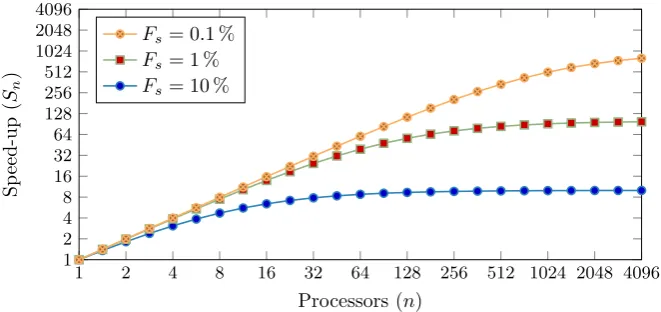
Amdahl’s law states that parallel speed-up is limited for all codes withfs>0,
even given access to an unlimited number of processors. Figure 2.3 shows how
the speed-ups given by Equation 2.9 quickly reach a plateau even for codes with
relatively tiny (fs= 0.1 %) serial portions.
Figure 2.4 illustrates an important corollary of Amdahl’s law. The parallel
efficiency (given by Equation 2.5) of any code with a serial portion will always
decrease as more processors are added.
Amdahl’s law only takes two parameters, yet despite this simplicity it is able
to provide valuable insights into application scalability. If application
perfor-mance follows Amdahl’s law at high processor counts then serial code is the
biggest barrier to scalability. Conversely, if observed performance is worse than
predicted, then parallel overhead is likely to blame.
Amdahl proposed his law in 1967 to demonstrate “the continued validity of
the single processor approach and of the weaknesses of the multiple processor
approach” [8]. Despite this, the multiple processor approach went on to become
1 2 4 8 16 32 64 128 256 512 1024 2048 4096 1
2 4 8 16 32 64 128 256 512 1024 2048 4096
Processors (n)
Sp
eed-up
(
Sn
)
Fs= 0.1 %
Fs= 1 %
[image:40.595.131.462.177.333.2]Fs= 10 %
Figure 2.3: Amdahl’s Law Speed-up Limits
1 2 4 8 16 32 64 128 256 512 1024 2048 4096
0.1 0.2 0.3 0.4 0.5 0.6 0.7 0.8 0.9 1
Processors (n)
Efficiency
(
En
)
Fs= 0.1 %
Fs= 1 %
Fs= 10 %
[image:40.595.137.456.479.633.2]Gustafson resolved this apparent paradox by observing that problem sizes
tend to grow to fill the available computing power [47]. This is because for
many HPC codes larger data sets translate to improved resolution, accuracy
or scale. Scientific computing workloads typically involve a serial setup phase
followed by repeatedly performing the same calculation on each element of a
dataset in parallel [9]. Most of the extra work associated with larger data sets
can be parallelised, meaning Wp increases faster than Ws. A smaller fraction
of runtime is spent on serial code when this observation holds, and speed-ups
improve as a result.
Amdahl’s and Gustafson’s laws are both valid, and the choice of which to use
depends on circumstances. That said, performance engineers are often tasked
with optimising code for a specific platform and problem size. They cannot rely
on arbitrarily large problem sizes and processor counts, and are therefore bound
by the limits of Amdahl’s law in most cases.
Amdahl’s and Gustafson’s laws only consider perfect parallelism, which
ap-plies when tasks can be executed independently and in any order. Imperfect
parallelism happens when dependencies impose partial orderings on the tasks
performed by a parallel algorithm. While tasks in the same sequence must be
executed in order, multiple independent sequences can be processed in parallel.
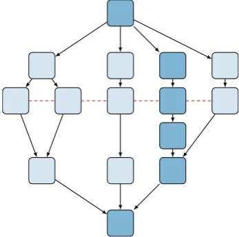
The work-span model represents algorithms as a set of tasks connected by
their dependencies to form a Directed Acyclic Graph (DAG). TimeT1 is called
an algorithm’s work; the cumulative runtime of all its sub-tasks. Time T∞ is
called an algorithm’sspan; the total runtime of itscritical path. The critical path
is the longest chain of tasks which must be executed sequentially. Algorithms
can never run faster thanT∞, even with access to unlimited processors.
Figure 2.5 shows an example of the work-span model in which all tasks take
unit time. This example does 15 units of work, one for each task, and has a
span of 6, one for each task on the critical path highlighted.
Figure 2.5: Work, Span and Maximum Cut
ratio ofT1andT∞provide the upper bound to speed-up shown by Equation 2.10:
Sn≤ T1
T∞ (2.10)
The bound given by Equation 2.11 comes from examining the best case scenario,
that allT1−T∞work off the critical path can be perfectly parallelised.
Tn ≥ T∞+T1−nT∞
⇔ Tn ≥ T1+ (n−1)T∞
n
∴ Sn ≤ n T1
T1+ (n−1)T∞ (2.11)
Work span DAGs can also be used to find the maximum degree of parallelism
exhibited by an algorithm. The maximum cut of the DAG (or more precisely
of its conjugate, i.e. cutting across nodes rather than edges) corresponds to the
largest number of tasks which can be executed concurrently. The red dashed
line in Figure 2.5 shows that at most 5 processors can be kept active at any one
time. Any processors added above this limit will remain idle.
Roofline is a more recent heuristic model which frames application
0.5 1 2 4 8 16 32 64 1
2 4 8 16 32 64 128
Peak FP Performance
TLP + ILP
TLP
Peak Bandwidth
HW Prefetc
h
No Prefetc
h
Operational Intensity (FLOPS/Byte)
P
erformance
(GFLOPS
[image:43.595.179.413.128.319.2])
Figure 2.6: Example Roofline Model
and floating point performance [121]. Operational intensity, the ratio between
work done and memory traffic, is then used to determine whether a code is
compute or memory bound.
Figure 2.6 shows an example of the Roofline model. Horizontal lines
corre-spond to floating point performance limits and diagonal ones to memory
band-width limits. A Roofline consists of one performance and one memory limit.
Platforms can exhibit many different Rooflines depending on which hardware
performance features can be used.
The Floating Point (FP) limits shown in Figure 2.6 are: Thread Level
Par-allelism (TLP), corresponding to the maximum performance of simple
multi-threaded programs; TLP plus Instruction Level Parallelism (ILP), the
maxi-mum performance of multi-threaded programs which use hardware features like
SIMD vectorization; and peak floating point performance, the maximum
perfor-mance of threaded, vectorised programs with the right instruction mix to keep
CPU functional units fully occupied.
The memory bandwidth limits shown in Figure 2.6 are: no prefetching,
0.5 1 2 4 8 16 32 1 2 4 8 16 32 64 128
Operational Intensity (FLOPS/Byte)
P erformance (GFLOPS) 0 25 50 75 100 125 150 175 200 225 250 275 P ow er (W ) Roofline Powerline
Figure 2.7: Powerline Model
hardware prefetching, whereby hardware is able to predict upcoming memory
accesses and preload the data; and peak bandwidth, the maximum possible
bandwidth attainable with perfect hardware prefetching and optimal memory
layout and access patterns.
Roofline models are able to diagnose performance issues using easily
obtain-able information. Developers identify where their code appears on a Roofline
diagram by measuring its operational intensity and floating point performance.
This allows them to determine which performance limit their code is bounded
by, and hence whether to look for runtime or memory optimisations.
In the example shown by Figure 2.6, improving the memory performance of
codes with operational intensities above eight FLOPS per byte will not reduce
their runtime. Even the lowest bandwidth limit is enough to keep a CPU fully
supplied with data beyond this point. Conversely, memory bandwidth should
be the sole optimisation target for codes with operational intensities under one
FLOPS per byte. Between these limits the best course of action depends on the
level of floating point performance observed.
condi-tions necessary for trade-offs between runtime and energy [19]. Figure 2.7 shows
the distinctive shape of their ‘Powerline’ model and how it compares to
conven-tional Roofline analysis. In particular, it shows how power consumption peaks
when operational intensity places equal demands on memory and floating point
performance. This is because with both subsystems under equal load, neither
one can become a bottleneck and force the other to enter an idle state waiting
for more work. Idle subsystems draw less power, so power consumption drops
off when either subsytem is forced to spend periods of time idle.
The Power Optimised Software Envelope (POSE) model developed in
Chap-ter 5 is another example of energy-aware heuristic performance modelling.
2.6.2
Analytical Modelling
Analytical models distil the structure and behaviour of a program into a set
of parameterised mathematical expressions. Performance predictions are then
obtained by solving these expressions for the required input parameters.
Ana-lytical models are able to predict the behaviour of real systems in a short amount
of time, making them particularly suitable for parameter studies.
Early analytical modelling approaches created bespoke models specific to
individual machines and applications. These approaches fell out of favour
be-cause of the considerable time and expertise required to model complex systems
accurately. Furthermore, the resulting models were not portable and had to be
completely rebuilt for each new platform. Modern approaches provide
gener-alised model skeletons which can be tailored to individual applications.
The Parallel Random Access Machine (PRAM) framework was one of the
first modelling techniques to produce portable performance models. PRAM
defines an idealised representation of SMP hardware consisting ofnprocessors
with perfectly synchronised clocks [40], as shown in Figure 2.8. Each processor
has its own private memory and can access global shared memory through a
common memory access unit. Processors perform one instruction each clock
Processorn
.. . Processor 2 Processor 1
Memory Access Unit
(MAU)
Global Shared Memory
Figure 2.8: PRAM Abstract Machine Model
Conflict resolution policies define what happens when multiple processors
ac-cess the same memory location simultaneously. There are four policies to
choose from, namely: Exclusive Read Exclusive Write (EREW), Concurrent
Read Exclusive Write (CREW), Exclusive Read Concurrent Write (ERCW),
and Concurrent Read Concurrent Write (CRCW). Both ERCW and CRCW
have sub-policies to determine which concurrent write access succeeds.
The PRAM model assumes that all processors are synchronised and
commu-nication between processors is free. These were reasonable assumptions when
uniform memory access SMP machines were common in HPC. The scalability of
these systems is limited by resource contention, however, and they have largely
been replaced by NUMA and message-passing DMM approaches.
PRAM emphasised the importance of model portability, however its models
are limited to SMP machines. The LogP model was devised to model parallel
applications regardless of the computer architecture used [24].
LogP is named after its four system parameters: L, which models network
latency; o, the overhead of sending and receiving messages; g, the minimum
gap between messages, or equivalently the reciprocal of inter-node bandwidth;
and P, the number of processors or nodes. LogGP extends the original model
messages and bulk transfers on many systems [6].
Some analytical models use hardware performance counters to estimate
sys-tem power consumption. Power usage and performance events are recorded for
a selection of benchmark programs. Regression analysis is then used to derive
power costs for each category of performance event. This approach has been
used to develop power models for components like CPUs [14, 69], GPUs [62],
and Xeon Phi coprocessors [111], as well as entire supercomputer systems [13].
Despite its popularity, this approach has significant limitations. Processors
can only monitor a small number of performance counters simultaneously, so
many events will be missed. Furthermore, processor events are not
standard-ised between processors, limiting the portability of these models. Lively et
al. demonstrated this fact and proposed code-specific power models as a
solu-tion [86]. In effect, they suggested intensolu-tionally over-fitting models to particular
target applications and platforms.
2.6.3
Simulation
Analytical performance modelling involves constructing detailed models of
ap-plication behaviour. Every apap-plication requires its own customised model, even
with modern frameworks, and these models must be continually updated and
revalidated in response to code changes. Simulators avoid these issues by taking
applications themselves as input, either directly or in the form of profiler traces.
Simulators gather performance data by running some representation of the
target application through a detailed model of a computer system. This shifts
the burden of model construction and verification away from performance
engi-neers and towards simulator designers. Once validated, a simulator can be used
to model the performance of many different applications.
Simulators are categorised based on the granularity of their system models.
Hardware simulators model the low-level operation of computer systems in as
much detail as possible. Cycle-accurate simulators are able to mimic hardware
designing new hardware or assessing the impact of exotic architectures.
Discrete event simulators operate at a higher level of abstraction, modelling
system behaviour as a sequence of distinct states. State transitions are triggered
by application events like network communications or synchronisation barriers.
Profilers gather event traces for a target application, which are then passed
as input to the simulator. Discrete event simulators are useful for ‘what if’
investigations which assess the likely outcomes of different scenarios.
Simulations are the most detailed approach to performance modelling, but
this detail comes at significant runtime cost. Event-based approaches require
traces to be gathered by running the original application in full. Hardware
ap-proaches take even longer as they run every application instruction through
sim-ulated hardware. Simulators like Sandia’s Structural Simulation Toolkit (SST)
offer a combined approach, providing hardware simulation for key components
and falling back to an event based approach where less detail is required [67].
Hardware simulation is often used to model power consumption. Wattch is
a popular framework for analysing and optimising microprocessor architectures
for reduced power consumption [17]. McPAT is a similar tool which replaces
the linear scaling assumptions in Wattch with non-linear power models, making
it suitable for the post-Dennard era [85].
SST supports system power simulation via its modular architecture [64].
Ex-isting component-level power simulators like McPAT are used as back-ends to
model the power consumption of individual processors, which SST then
aggre-gates to provide a system-level overview.
2.7
Optimisation
Performance optimisation involves modifying applications to improve properties
like runtime or energy consumption. Algorithmic optimisationslead to more
effi-cient algorithms irrespective of the platform used. Once these optimisations are

![Figure 3.1: Power Density Trends, based on data from [22]](https://thumb-us.123doks.com/thumbv2/123dok_us/9460635.452777/53.595.194.395.122.366/figure-power-density-trends-based-data.webp)