A. Optimization Model Based on Dynamic Programming



Abstract—The efficient design of water transmission main involves several optimization processes among which an important place is held by their path optimization. In this paper are developed two deterministic mathematical models for optimization of water transmission main path, based on techniques of sequential operational calculus, implemented in a computer program. Using these optimization models could be obtained an optimal solution for selection of source location and of water transmission main path based on graph theory and dynamic programming. The results of few numerical applications show the effectiveness and efficiency of the proposed optimization models.

Index Terms—dynamic programming, graph theory, optimal path, optimization models, water transmission main.

I. INTRODUCTION

HE water transmission mains have a significant importance in water supply systems due to their large investment amount and important energy consumption [1]. As a consequence, the efficient design of water trans-mission main involves several optimization processes among which an important place is held by their path optimization.

In current design practice, the choice of the optimal solution is made usually through analytical study of two or three versions selected from the possible set by predicted decisions [2]. The errors of these decisions are inverse proportional to the designer experience.

The modern mathematical disciplines as operational research give to the designer a vast apparatus of scientific analysis in optimal decisions establishing [3]-[9]. The mathematical theory and planning of multistage decision processes, the term was introduced by Richard Bellman in 1957 [10, 11]. It may be regarded as a branch of mathe-matical programming or optimization problems formulated as a sequence of decision.

Dynamic programming is useful however for optimizing temporal processes such as those typical in system operation problems. Sterling and Coulbeck [12], Coulbeck [13], Sabel and Helwig [14], and Lansey and Awumah [15] applied

I. Sarbu is with the Department of Building Services, “Politehnica” University of Timisoara, 300006 Timisoara, Romania (corresponding author to provide phone: +40256403991; fax: +40256403987; e-mail: ioan.sarbu@ ct.upt.ro).

E. S. Valea is with the Department of Building Services, “Politehnica” University of Timisoara, 300006 Timisoara, Romania (e-mail: [email protected]).

dynamic programming to determine optimal pumping operation for minimization of costs in a water system. Dynamic programming [16], [17] is also used primarily to solve tree–shaped networks and could be extended to solve to looped systems [18]. Also, Sarbu [19] has been applied graph theory to establish optimal path for branched water supply networks.

In this context, in this paper are developed two deterministic mathematical models for optimization of water transmission main path, based on techniques of sequential operational calculus, implemented in a computer program. Using these optimization models could be obtained an optimal solution for selection of source location and of water transmission main path based on graph theory and dynamic programming. The results of few numerical applications show the effectiveness and efficiency of the proposed optimization models.

II. OPTIMIZATION MODELS

A. Optimization Model Based on Dynamic Programming

Sequential decision problem stated above is typical of dynamic programming, which is a procedure for optimizing a multistage decision at each stage. The technique is based on the simple Bellman’s principle of optimality [11], [20], which states that “an optimal policy has the property that whatever the initial state and initial decision are, the remaining decisions must constitute an optimal policy with regard to the state resulting from the first decision.

To solve a dynamic programming problem, it is neces-sary to evaluate both immediate and long-term consequence costs for each possible state at each stage. This evaluation is done through the development of the following recursive equation (for minimization):

min ( ₁, )

1

i i N i

i X X

V

Z 





 (1)

considering that each size Xi can vary in a field that depends

on X0 and Xi+1 , i = 1, 2,..., N.…

Optimization formula (1) is generalized for case if the terms Xi are vectors with n components:

X_i 





variable variation domains allow use of a system of N

phases for which Vi (Xi-1, Xi); (i = 1, 2,..., N) is the value

function attached to each phase, and Z- value function attached for phase crowd.

Application of Operational Research to

Determine Optimal Path for a Water

Transmission Main

Ioan Sarbu and Emilian Stefan Valea

Finding the minimum of the function Z requires solving

at each step the functional equation:

min[ ( , ) ( , )]

) ,

( _{0 1 0, 1 0 1}

, 0

1   

 

 i i i i i

X i

i X X V X X f X X

f

i

(3) where the notation Xi–1 means that Xi–1 belongs to a values set which depend only on X0 and Xi.

Calculation procedure consists in successively solving of minimization problems (3) for i = 1, 2,..., N, with discrete

variation of X0 and storing intermediate results. Thus, it are calculated successive optimal sub-policies for phases 1 and 2 together, then phase 1, 2 and 3 together, ..., for phases

N

,

1 together, i.e. optimal policies:

  ) , ( ) , ( [ min ) , ( min 1 0 1 , 0 1 0 , 0 1         N N N N N X N N X X f X X V X X f Z

n (4)

in which f0,N(X0,XN)is optimal policy value from X0 to XN;

VN(XN-1,XN) – sub-policy value from XN–1 to XN; f0,N–1(X0,

XN–1) – optimal policy value from X0 to XN–1.

A numerical example which illustrates the application of this optimization model shall be presented below.

B. Optimization Model Based on Graph Theory

Mathematical model of dynamic processes of discrete and, determinist type can be simplified using graph theory. The modeling of stated problem is realized by plotting oriented connected graph G = (X, U) which consists of

source as origin, paths as edges and critical points as vertices. Each edge uijU is assigned with a number

0 ) ( i 

j

u

 , in conventional units, depending on the adopted optimization criterion. Optimal path is given by minimum value path in the graph, which is determined by applying the Bellman-Kalaba algorithm [2], [21].

The graph G = (X, U) has attached a matrix M whose

elements mij are:

           . r f 0 ; adjacent not are and vertices if ; to from value edge ) ( j i o x x x x u

m _{i j}

j i i j ij  (5)

Optimal path is given by path  of graph, which has the total value:







u ) min (

) μ

( (6)

If Vi is the minimum value of existing pathμ ,(i 0,n) i

n 

from at vertex xi to vertex xn:

Vi 



V_n 0 (8) then in accordance with the principle of optimality:

0 and ) 0, ; 1 0, ( , )

min(     



i ij n

j j

i V m i n j n V

V (9)

The system (9) is solved iteratively, noting with k i

V the

value of Vi obtained from iteration k, namely:

o _ ( _0, _1); o_0

n in

i m i n V

V (10)

It is calculated:

0 ; ) 0, ; 1 0, ( , )

min( o 1

1_{     }

i ij n

j j

i V m i n j n V

V (11)

and then: 0 ; ) 0, ; 1 0, ( , )

min( 1_{    }

   k n i j ij k j k

i V m i n j n V

V (12)

Order k of iteration expressed by (12) gives finite values

only for paths with length at most k-1, arriving at xn,

choosing between them minimal ones. From ones iteration to the next:

1 .

j , V

V_ik  _ik  (13) Numbers V_ik(in;k0,1,...) form monotone decreasing strings that necessarily reach a minimum after a finite number of iterations that not exceed n-1. So, the

algorithm stops when it comes to an iteration k such that

, 1   k i k i V

V (i0,n) and the value of the minimum path

between vertex. x0 and xn is V0k V0k1.

In order to identify the paths that have found minimum values, shall be deducted from (12) that along them, at the last iteration: k j ij k j ij k

i m V m V

V   1  (14) Based on the described optimization model a computer program OPTRAD was performed in Fortran programming language for PC compatible microsystems, with the flow chart shown in Figure 1, where: N is the graph order; M(I,J)

– matrix associated to the graph; V(I,J) – column vector

built for each iteration k; X(I) – vertices succession of path

with minimum value; VAL – value of the minimum path in

graph..

Bellman-Kalaba algorithm is not but the expression in another language of the optimality principle and analytical procedure for applying functional equations (3) and (4) is only a special case, more elementary of this algorithm.

C. Sensitivity of Optimal Solution

At a complex analysis that involve several optimization criteria in a sequentially program, is necessary to determine the optimal solution sensitivity. Exploration of optimal solution neighborhoods leads to the problem of k-optimal solutions, i.e. at the determination of the solutions very closed of optimal one (quasi optimally).

Fig. 1 Flow chart of computer program OPTRAD

III. NUMERICAL APPLICATIONS

A. Application of Optimizing Model Based on Dynamic Programming

For example, a water transmission main for a village L starting from two source locations S1 and S2 is considered (Fig. 2). Possible paths pass through critical points A, B, C, D, and E, forming three sectors. Could be applied dynamic programming model to solve the selection problem of source location and of the path for this water transmission main.

Fig. 2 Variants of adduction path

Adopting as optimization criterion the minimum total investment cost, partial investment is determined for each path and sequentially graph is plotted in Figure 3. In this graph each edge have associated a cost in conventional units. They noted with X0, X1, X2 and X3 decision variables related to the each sector. These variables will not take numerical values, but will be vertices in that graph which are on the same alignment.

Fig. 3 Sequential graph of possible adduction paths

The cost of sector 1 is noted VI (X0, X1). This depends on values of X0 and X1 (in this case, X0 could be only L). Identically are noted VII (X1, X2) and VIII (X2, X3).

The total value of adduction system is expressed by:













I X ,X V X ,X V X X V

Initially, the transmission main is considered developed on a single sector (I). Noting with fI(X1) the minimum cost of sector I, for each of critical points A, B, C, equation (3) becomes: 6 ) , ( ) ( ; 9 ) , ( ) ( ; 8 ) , ( ) ( I I I I I I       C L V C f B L V B f A L V A f (16) The operator ”min” is missing because step zero does not exist.

It is considered that the transmission main is formed of two sections (I, II), is denoted by fI, II(X2) the minimum cost for sectors I and II together, for different values of X2 equation (3) becomes:





 









 





, , II I, 1 I 1 II , , II I, , min ) ( , min ) ( 1 1 X f E X V E f X f D X V D f C B A X C B A X       (17)

Giving successively to X1 the values A, B, C and taking into account that for inexistent links are considered ∞ value, from previous relationships results:

C X E f A X D f C X B X A X C X B X A X                    1 II I, 1 II I, for , 15 ] 6 9 , 9 6 , 8 8 min[ ) ( ; for , 15 ] 6 , 9 7 , 8 7 min[ ) ( 1 1 1 1 1 1 (18)

At the last step is considered that the transmission main is developed on sectors I, II, and III. According with optimality principle the minimum cost for sectors I, II, and III together, corresponding to values S1 and S2 for X3, is written as:

 





 

 





 

III II, I, 2 II I, 1 2 III , 1 III II, I, , [ min ]; , [ min 2 2 X f S X V S f X f S X V S f E D X E D X       (19)

obtaining for the given example:

 

 

f D X S f E X D X E X D X I                2 2 III II, I, 2 1 II II, I, for , 21 ] 15 6 , 15 min[ ; for , 19 ] 15 5 , 15 4 min[ 2 2 2 2 (20)

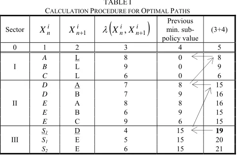
Results as optimal solution the source location in S1 and the water transmission main path: S1, D, A, L. Because of the analytical computation procedure is less intuitive, a calculation procedure in table is presented. So, in Table 1 are shown in column 0 the sector, in column 1 the vertex which marks the start of sector, in column 2 the vertex which marks the end of sector, in column 3 the value of corresponding edge, in column 4 the value of previous minimum sub-policy, and in column 5 the sum of columns 3 and 4.

After fulfilling the entire table, is read the minimum value from column 5 of the sector III, which is 19, the bolded number. From this, it starts with a horizontal arrow to column 4 and is obtained 15; from here it starts again back in column 5 and up, to the position where he was transferred this number, and so on. The arrows show the optimal solution. The path is read from the column 1 with the first vertex S1, continue in column 2 on the position of horizontal arrow: S1, D, A, L (vertices that were underlined in table).

TABLEI

CALCULATION PROCEDURE FOR OPTIMAL PATHS

Sector i n

X X_ni1





i n X

X , 1

 min. sub-Previous policy value

(3+4)

0 1 2 3 4 5

I

A L 8 0 8

B L 9 0 9

C L 6 0 6

II

D A 7 8 15

D B 7 9 16

E A 8 8 16

E B 6 9 15

E C 9 6 15

III

S1 D 4 15 19

S1 E 5 15 20

S2 E 6 15 21

After fulfilling the entire table, is read the minimum value from column 5 of the sector III, which is 19, the bolded number. From this, it starts with a horizontal arrow to column 4 and is obtained 15; from here it starts again back in column 5 and up, to the position where he was transferred this number, and so on. The arrows show the optimal solution. The path is read from the column 1 with the first vertex S1, continue in column 2 on the position of horizontal arrow: S1, D, A, L (vertices that were underlined in table).

B. Application of Optimizing Model Based on Graph Theory

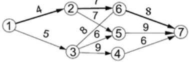
It is presented a numerical example of application of optimizing model based on the graph theory to determine the optimal path of water transmission main for village L, starting from source S1.

It is plotted in Figure 4, the oriented connected graph of order n = 7, formed of source as origin, paths as edges and

critical points as vertices.

Fig. 4 Graph of adduction paths

The matrix M assigned to graph has the elements mij

defined with (5):

                                                       0 8 0 9 0 6 0 8 6 9 0 7 7 0 5 4 0

M (21

Using computer program OPTRAD it was determined minimum path in graph: (1, 2, 6, 7), having the value 19. It results that the optimal path of water transmission main is

IV.CONCLUSION

In the presented optimization models were described two techniques for solving sequential programs. Applying the dynamic programming in determinist case for built of a transmission main can be established optimal path from more possible variants. The elaborated computer program based on the graph theory, for compatible microsystems, allows performing a quick and efficient computation.

REFERENCES

[1] T. M. Walski, D. V. Chase, D. A. Savic, W. Grayman, S. Beckwith, and E. Koelle, Advanced Water Distribution Modeling and Management, Waterbury, USA, Haestad Press, 2003.

[2] I. Sarbu, Numerical Modeling and Optimization in Building Services (in Romanian), Timisoara, Politehnica Publishing House, 2010.

[3] A. Kaufmann, Methods and Models of Operations Research, Englewood Cliffs, N.J., Prentice Hall Inc., 1963.

[4] A. Stefanescu and C. Zidaroiu, Operational Researches (in Romanian), Bucharest, Teaching and Pedagogical Publishing House, 1981.

[5] L. R. Foulds, Graph Theory Applications, New York, Springer-Verlag, 1992.

[6] J. L. Gross and T. W. Tucker, Topological Graph Theory, Portland, John Wiley & Sons, 2001.

[7] R. Diestel, Graph Theory, New York, Springer-Verlag, 2005. [8] E. Polak, Computational Methods in Optimization, New

York, Academic Press, 1971.

[9] S. Pemmaraju and S. Skiena, Computational Discrete Mathematics: Combinatory and Graph Theory with Mathematics, Cambridge, Cambridge University Press, 2003.

[10]S. Dreyfus, “Richard Bellman on the birth of dynamic programming”, Operations Research, vol. 50, no. 1, pp. 48-51, 2002.

[11] R. E. Bellman, Dynamic Programming, New York, Dover Publications, 2003.

[12]M. J. Sterling and B. Coulbeck, “A dynamic programming solution to optimization of pumping costs”, Proceedings of Institute of Civil Engineers,vol. 59, no. 2, pp. 813, 1975. [13]B. Coulbeck, “Optimization of water networks”, Transactions

of Institute of Measurements and Control, vol. 6, no. 5, pp. 271, 1984.

[14] M. H. Sabel and O.J. Helwing, “Cost effective operation of urban water supply system using dynamic programming”, Water Resources Bulletin, vol. 21, no. 1, pp. 75, 1985. [15]K. E. Lansey and K. Awumah, “Optimal pump operation

considering pump switches”, Journal of Water Resources Planning and Management, ASCE, vol. 120, no. 1, pp. 17, 1994.

[16]T. Liang, “Design conduit system by dynamic programming,” Journal of Hydraulics Division, ASCE, vol. 97, no. HY3, pp. 383-393, 1971.

[17]K. P. Yang, T. Liang, and I.P. Wu, “Design of conduit system with diverging branches”, Journal of Hydraulics Division, ASCE, vol. 101, no. HY1, pp. 167-188, 1975.

[18]Q. W. Martin, “Optimal design of water conveyance systems”, Journal of Hydraulics Division, ASCE, vol. 106, no. HY9, 1980.

[19]I. Sarbu, “Path optimization of a branched water supply network” (in French), Scientific Bulletin of I P Timisoara, Romania, vol. 42, no. 1, pp. 120-127, 1997.

[20]R. Bellman, Methods of Nonlinear Analysis, London, Academic Press, Inc., 1973.