Abstract— This paper demonstrates a mathematical model of a repairable spinning solution preparation system, a part of an acrylic yarn manufacturing plant with an attempt to improve its availability. The methodology for determining the availability of the system is based on Markov Modeling. The failure rates of the different subcomponents of the system are taken as constant while their repair times are arbitrarily
distributed. Probability considerations and
supplementary variable technique are used in
formulation of the problem. Lagrange’s method for partial differential equations is used to solve system governing equations. The reliability characteristics are evaluated in accordance with practical situation and operational behavior of the system is analyzed. Availability analysis of the system helped in identifying the contributing factors and assessing their impact on the system availability.
Index Terms— availability, steady state availability, maintainability, mission reliability
I. INTRODUCTION
ODAY with competition in industry at an all time high, reliability of process plants has become a big concern for the manufacturers. Process reliability and availability gives us the necessary information for improving the system productivity and optimizing the cost of production and maintenance.
In recent past, researchers have recognized to derive more benefits in terms of higher productivity and lower maintenance costs with the application of reliability/availability/maintainability engineering in manufacturing industries. Dyer D. [1] analyzed the unification of Reliability/Availability/ Repair-ability models for Markov system. Kumar D. et all [2] used Markovian approach to model the process of feeding system a component of sugar industry for its production improvement. Islamov R. T. [3] proposed a general method for determining the reliability of multiple repairable systems. The kolmogorov equations with a large number of differential equations are transformed into integral differential equations to obtain solutions. Microelsen Q. [4] has described the status of the use of reliability technology in the process industry for the present time and how to proceed for future. Tsai Y. et al [5] presented a method to
P. Gupta is working as Professor with Mechanical Engineering Department of Sant Longowal Institute of Engineering and Technology, Longowal, Punjab, India (e-mail: [email protected]).
study the effect of three types of PM actions – mechanical service, repair and replacement on availability of a multi-component system. Gupta P. et al [6] derived some interesting reliability characteristics and obtained optimum number of maintainers to maintain 14 spinning cells of a 7-Out-of-14: G chemical system. Sharma R.K. and Kumar S. [7] used RAM analysis on a urea production process plant with an aim to minimize its failures, plant maintainability requirements and optimize equipment availability. Guo H. et al [8] applied a more general mathematical model and algorithms for the reliability analysis of wind turbines. A three parameter weibull failure rate function is used to model the problem and the parameters are estimated by maximum likelihood and least squares. Umemura and T. Dohi [9] analyzed the stochastic behavior of an electronic system through an embedded Markov Chain approach in continuous-time and discrete-time scales with the purpose to maximize its steady-state availability. Several methods have been proposed by reliability practitioners for reliability/availability analysis of industrial systems under different working conditions which can benefit the industry in a number of ways.
In this paper a real life and complex repairable spinning solution preparation system, a part of an acrylic yarn manufacturing plant is considered for the availability analysis. Probability considerations and supplementary variable technique are used in formulation of the problem. Lagrange’s method for partial differential equations is used to solve system governing equations. Numerical results based upon the true data collected from industry are presented to illustrate the steady state behavior of the system under different plant conditions. The results obtained are very informative and can also help in improving the operational availability of the system.
II. SYSTEMDESCRIPTION
The spinning solution preparation system consists of five subsystems: A, B, C, D, & E working in series. This system prepares spinning solution from dry polymer powder which is supplied to it by Polymer Powder Production System. The flow diagram representing working of this system is shown in figure-1. The variable screw feeder discharges dry polymer powder to mass flow meter and this regulates the polymer powder flow. This powder flows by gravity to a spray chamber, where polymer powder is wetted by a metered flow of Dimethyl Formamide (DMF) containing DTPA & TiO2 as desired. A heater is provided on the DMF
line to achieve the desired mixing temperature. The polymer wetted out with solvent then passes through a screw type mixer for thorough mixing, which also transfer this well mixed solution to a jacketed blend tank where an agitator blends out mixing irregularities before it discharged into the
Markov Modeling and Availability Analysis of
a Chemical Production System-A Case Study
Pardeep Gupta, Member IAENG
solution storage tank. This solution storage tank serves the dual purposes: it supplies the solution continuously, and goes on accumulating buffer solution which it can supply for about four hours in case any unit/subsystem poisoned prior to the solution storage tank breaks down. The solution from storage tank is pumped to solution heater with the help of gear pumps. Next the solution from solution heater goes to the filter presses (FPs), which are six units working in parallel for removing impurities and un-reacted polymer. Finally the filtered spinning solution is pumped to the spinning area for its next continued processing.
Dry Polymer Powder Dry Polymer Powder
Buffer
Stock
Spinning solution Fig. 1. Process Flow Diagram
The following notations and assumptions are addressed for the purpose of mathematical analysis of availability of the system.
III NOTATIONS AND ASSUMPTIONS A NOTATIONS
Subsystem A: consists of two identical items (
A
i,
i
=
1
,
2
) working in parallel. Each item further consists of two units: spray chamber & screw type mixer working in series. On failure of its one unit A1 or A2, the full system will work withfull capacity upto four hours as the storage tank (subsystem-C) can supply the extra buffer solution for this duration of time. But in case the repair is not completed within the target time, the system will start working under reduced capacity. Subsystem B: consists of one unit namely blend tank subjected to major failures only.
Subsystem C: consists of one unit namely solution storage tank which can supply the extra stored solution upto four hours and it never fails.
Subsystem D: consists of two identical solution heaters, one is in working state and another is in standby state. Thus this subsystem never fails.
Subsystem E: consists of six identical filter presses (Ei ,i
=1,2,..,6). Out of six units, normally one press remains under either preventive maintenance (PM) or corrective maintenance (CM) and the system with the rest of five presses works at full capacity. As timely scheduled PM and prompt CM is initiated, it is appropriate to assume that at the most two presses may remain under PM and CM in parallel. With four presses the system works at reduced capacity. o : subsystem/component is operative.
g : subsystem/component is good but not operative. d : subsystem/component is working in degraded state on failure of its one unit and the failed unit is under repair.
r : subsystem/component is under repair.
m m
i i
A
,3,− : indicates the working of the partsA
i &A
3−i pertaining to subsystem A ( i = 1,2 ; m = o, g , r).The ordered pairs (mi ) and (3m−i) refer the status of the partsA
i &A
3−i with respect to m.m m
j j
A
,3,− : identical toA
im,3,−mi, and j = i, i.e. j is assigned the same index as is assigned to i in state-1n
X
: (X = B, E; n=o,g,r,d,φ
whereφ=o,g) representsthe status of the subsystems B and E with respect to n.
i
λ
: refers respective failure rate of itemsA
1 &A
2. Eachi
A
consists of two unitsA
i1 &A
i2 (working in series) and having failure ratesλ
i1 andλ
i2 such thatλ
i=λ
i1+λ
i2, ( i= 1, 2) .
k
λ
: refers respective failure rate of the units B and E, (k=3, 4).( )
x
i
µ
,η
i( )
x
: refer respective repair rate and pdf of repair time of the units/subsystems A1, A2, B and E, and has anelapsed repair time x , ( i = 1,2, 3, 4).
( )
t
P
0 : probability that the system is operating with full capacity at time ‘t’.( )
x
t
P
i,
: probability that the system is in state ‘i’ at time ‘t’ , and has an elapsed repair time x, ( i = 1,2,…., 8).( )
t
Q
: probability of the system being in failed state at time ‘t’ conditioned that t › τ, where τ is the mission repair time.M
( )
τ
;
t
: mission reliability function.B ASSUMPTIONS
i All the units are initially operating and are in good state. ii) Each unit has two states viz., good and failed
iii) Each unit is as good as new after repair.
iv) The failure rates are constant and the repair times are arbitrarily distributed.
v) Failure and repair events are statistically independent. vi) Whenever a unit fails its repair begins immediately. vii) Concurrent repair can takes place when more than two subsystems are in failed states as independent repair facilities are available for individual subsystems. viii) Maximum two subsystems will come to failed states at the same time because repair of failed units begins immediately and is carried out quickly.
Spray Chamber (A11) Screw Type Mixer (A22)
Blend Tank (B)
Solution Heater (D)
Solution Storage Tank (C)
F P (E1) F P (E2) F P (En) , n =3,4,5 F P (E6)
Screw Type Mixer (A12)
The state transition diagram as shown in Fig. 2 is established using the above notations and assumptions, see Annexure-I
IV.
M
ATHEMATICALA
NALYSISO
FT
HES
YSTEM Probability considerations give the following differential-difference equations associated with the transition diagram:( )
t T P( )
t S( )
t Pdt d
i
i 0 0
0
0 + = (1)
( ) ( )
x
P
x
t
S
( )
x
t
T
t
x
1i
1,
=
1i,
+
∂
∂
+
∂
∂
(2)( ) ( )
x
P
x
t
S
( )
x
t
t
x
3
2,
=
2i,
+
∂
∂
+
∂
∂
µ
(3)( ) ( )
x
P
x
t
S
( )
x
t
T
t
x
2i
3,
=
3i,
+
∂
∂
+
∂
∂
(4)( ) ( )
x
P
x
t
P
( )
x
t
T
t
x
3i
4,
=
3−i 1,
+
∂
∂
+
∂
∂
λ
(5)( ) ( )
x
P
x
t
P
( )
x
t
T
t
x
4i
5,
=
λ
3 1,
+
∂
∂
+
∂
∂
(6)( ) ( )
x
P
x
t
P
( )
x
t
P
( )
x
t
T
t
x
5i
6,
=
λ
4 1,
+
λ
i 3,
+
∂
∂
+
∂
∂
(7)( ) ( )
x
P
x
t
( ) ( )
x
P
x
t
t
x
µ
3 i
7,
=
µ
i 4,
+
∂
∂
+
∂
∂
− (8)
( ) ( )
x
P
x
t
P
( )
x
t
T
t
x
6
8,
=
λ
3 3,
+
∂
∂
+
∂
∂
(9)( )
0
=
dt
t
dQ
for t ‹
τ
=
∫
( )
+
∫
∑
( )
+
∫
( )
= t t k k tdx
t
x
P
dx
t
x
P
dx
t
x
P
τ τ τ,
,
,
8 5 4 2for t ›
τ
(10) With initial and boundary conditions:( )
0
1
0
=
P
P
j( )
x
,
0
=
0
forj
=
1
,
2
,...,
8
( )
t
P
( )
t
P
10
,
=
λ
i 0P
2( )
0
,
t
=
λ
3P
0( )
t
( )
t
P
( )
t
P
30
,
=
λ
4 0P
4( )
0
,
t
=
λ
3−i∫
P
1( )
x
,
t
dx
( )
t
P
( )
x
t
dx
P
50
,
=
λ
3∫
1,
( )
t
P
( )
x
t
dx
P
( )
x
t
dx
P
60
,
=
λ
4∫
1,
+
λ
i∫
3,
( )
0
,
0
7
t
=
P
P
8( )
0
,
t
=
λ
3∫
P
3( )
x
,
t
dx
(11) Where( )
t( ) ( )
x P xtdx( ) ( )
xP xtdx( ) ( )
xP xtdxS0i =
∫
µi 1 , +∫
µ3 2 , +∫
µ4 3 ,( )
xt P( )
t( ) ( )
xP xt( ) ( )
xP xt( ) ( )
xP xt S1i , =λi 0 +µ3−i 4 , +µ3 5 , +µ4 6 ,( )
xt P( )
t( ) ( )
xP xt( ) ( )
x P xt S2i , =λ
3 0 +µ
i 5 , +µ
4 8 ,( )
xt P( )
t( ) ( )
xP xt( ) ( )
xP xtS3i , =λ4 0 +µi 6 , +µ3 8 ,
4 3 0i
=
λ
i+
λ
+
λ
T
( )
x
( )
x
T
1i=
λ
3−i+
λ
3+
λ
4+
µ
i( )
x
( )
x
T
2i=
λ
i+
λ
3+
µ
4( )
x
( )
x
( )
x
T
3i=
µ
i+
µ
3−i( )
x
( )
x
( )
x
T
4i=
µ
i+
µ
3( )
x
( )
x
( )
x
T
5i=
µ
i+
µ
4( )
x
( )
x
( )
x
T
6i=
µ
3+
µ
42
,
1
=
i
for all the above equations.A SOLUTION OF EQUATIONS:
Equation (1) is a linear differential equation of first order and other equations (2) - (9) are linear partial differential equations of first order. Solving the above system of equations yield the state probabilities:
( )
=
−[
+
∫
( )
]
dt
e
t
S
e
t
P
T0it i T0it0
0
1
(12)( )
( )(
)
( )
( ) − + ∫ ∫=e− P t x
∫
S x te dxt x
P T1ixdx i i T1ixdx
,
, 0 1
1 λ (13)
( )
( )(
)
( )
( ) − + ∫ ∫=e− P t x
∫
S xt e dxt x
P 3xdx i 3xdx
,
, 3 0 2
2
µ µ
λ (14)
( )
( )(
)
( )
( ) − + ∫ ∫=e− P t x
∫
S xte dxt x
P i T xdx
dx x
T2i 2i
,
, 4 0 3
3 λ (15)
( )
= ∫ ( ) (
−)
+∫
( )
∫ ( ) − − − dx e t x P x t P e t xP i i T xdx
dx x
T3i 3i
,
, 3 1 3 1
4 λ λ (16)
( )
( )(
)
( )
( ) − + ∫ ∫=e− P t x
∫
P x te dxt x
P T4ixdx T4ixdx
,
, 3 1 3 1
5 λ λ (17)
( )
( )(
)
(
)
[
P t x P t x]
e t x P i dx x Ti − + − ∫
= − 4 1 3
6
5
, λ λ
( )
( )
( )
(
)
( ) + ∫ ∫+e−
∫
P x t iP x t e T xdxdxdx x
T5i 5i
,
, 3
1
3 λ
λ (18)
( )
( )( ) ( )
( ) ∫ ∫ = − −∫
− dx e t x P x e t xP 3ixdx i 3I xdx
,
, 4
7
µ µ
µ (19)
( )
= −∫ ( ) (
−)
+∫
( )
∫ ( ) dx e t x P x t P e t xP T6xdx T6xdx
,
, 3 3 3 3
8 λ λ (20)
In the above state probabilities obtained, probabilities P4(.),
P5(.), P6(.) are given in terms of P1(.) & P3(.),and P7(.) and
P8(.) are given in terms of P4(.) & P3(.) respectively. After
substituting the values of P6(.) and P8 (.), equation (15) gives
the probability P3(.) in terms of P0(.) and P1 (.). On solving
equations (16)-(20) yield probabilities Pi (.), ( i = 4,5,…,8)
in terms of P0(.) and P1 (.). With substituting the values of P4
(.), P5 (.), and P6 (.) in terms of P0(.) and P1 (.), the equation
(13) gives the value of P1 (.) in terms of P0(.). Again on
solving the above equations, all probabilities Pi (.), ( i =
2,3,…,8) are obtained in terms of P0(.) which is given by
integral equation (12).
Equation-(10) on integration yields:
( )
∫ ∫
( )
∫ ∫∑
( )
∫ ∫
( )
+ + = = t t t t k k t t dt dx t x P dt dx t x P dt dx t x P t Q 0 8 0 5 4 02 , , ,
τ τ
τ
The expressions to determine mission reliability function M (τ ; t) and availability function A(t) are obtained as:
M (τ ; t) =
1
−
Q
( )
t
( )
∫ ∫ ∑
( )
∫ ∫
( )
∫ ∫
− − − = = t t t t k k t t dt dx t x P dt dx t x P dt dx t x P 0 8 0 5 4 02 , , ,
A (t) = 1 if t ‹
τ
=
P
( )
t
P
( )
x
t
dx
i i
∫ ∑
=+
7 , 6 , 3 , 10
,
if t ›τ
(22)The Mission Repairability Function (
MR
i) i.e. the probability of a system returning to operative state from critical states (i = 2,5,8) & 4 in some specified time ‘τ
’ are given by relations 23 & 24 respectively.( )
∫
=
τη
03
x
dx
MR
i , i = 2,5,8 (23)( )
∫
−=
τη
0 34
x
dx
MR
i , i = 1,2 (24)B SPECIAL CASES
:
a) STEADY STATE AVAILABILITY:
When t → ∞, →0
∂ ∂
t and dt
d equations (1) – (9) reduces to:
i i
P
S
T
0 0=
0 (25)( ) ( )
x
P
x
S
( )
x
T
x
1i
1=
1i
+
∂
∂
(26)( ) ( )
x
P
x
S
( )
x
x
3
2=
2i
+
∂
∂
µ
(27)( ) ( )
x
P
x
S
( )
x
T
x
2i
3=
3i
+
∂
∂
(28)( ) ( )
x
P
x
P
( )
x
T
x
3i
4=
3−i 1
+
∂
∂
λ
(29)( ) ( )
x
P
x
P
( )
x
T
x
4i
5=
λ
3 1
+
∂
∂
(30)( ) ( )
x
P
x
P
( )
x
P
( )
x
T
x
5i
6=
λ
4 1+
λ
i 3
+
∂
∂
(31)( ) ( )
x
P
x
( ) ( )
x
P
x
x
µ
3i
7=
µ
i 4
+
∂
∂
− (32)
( ) ( )
x
P
x
P
( )
x
T
x
6
8=
λ
3 3
+
∂
∂
(33)Solving recursively the above system of equations, we get the state probabilities:
( )
( )( )
( )
∫
∫
=
e
−∫
S
x
e
dx
x
P
T1i xdx i T1i xdx1
1 (34)
( )
( )( )
( )
∫
∫
=
e
−∫
S
x
e
dx
x
P
3xdx i 3xdx2 2 µ µ (35)
( )
( )( )
( )
∫
∫
=
e
−∫
S
x
e
dx
x
P
T2i xdx i T2i xdx3
3 (36)
( )
( )( )
( )
∫
∫
=
e
− −∫
P
x
e
dx
x
P
T3i xdx i T3i xdx1 3
4
λ
(37)( )
( )( )
( )
∫
∫
=
e
−∫
P
x
e
dx
x
P
T4i xdx T4i xdx1 3
5
λ
(38)( )
= −∫ ( ) ∫
(
( )
+( )
)
∫ ( ) dx e x P x P e xP T5ixdx i T5i xdx
3 1
3
6
λ
λ
(39)( )
( )( ) ( )
( )
∫
∫
=
− −∫
−dx
e
x
P
x
e
x
P
3i xdx i 3 I xdx4 7
µ µ
µ
(40)( )
( )( )
( )
∫
∫
=
e
−∫
P
x
e
dx
x
P
T6 xdx T6 xdx3 3
8
λ
(41)Arranging as in previous section , all the probabilities Pi(.) , i
= 1,2,…,8 are obtained in terms of ‘P0’ which can be
obtained using the normalizing condition i.e., the sum of all the probabilities is equal to one. The steady state availability of the system (
A
SS) in case repair time of subsystem-B exceeds mission time is given by:( )
∫ ∑
=+
=
7 , 6 , 3 , 1 0 i iSS
P
P
x
dx
A
(42)b) STEADY STATE AVAILABILITY WITH CONSTANT TRANSITION RATES:
The state probabilities are obtained as:
0
P
M
P
i=
i For i = 1, 2,…,8Where
4 3 0i
=
λ
i+
λ
+
λ
T
i i
i
T
1=
λ
3−+
λ
3+
λ
4+
µ
4 3 2i
=
λ
i+
λ
+
µ
T
i i i
T
3=
µ
+
µ
3−3 4i
=
µ
i+
µ
T
4 5i
=
µ
i+
µ
T
4 3 6i
=
µ
+
µ
T
6 3 3 5 2 1T
T
T
K
i i i iµ
λ
µ
λ
−
−
=
+
+
−
−
=
− − i i i i i i i i i iT
T
T
K
T
T
T
K
5 4 4 3 3 3 3 3 1 5 4 5 4 4 1 2µ
λ
µ
λ
µ
λ
µ
λ
µ
λ
+
+
+
=
− − i i i i i i iT
T
T
K
K
M
5 4 4 3 3 3 3 3 1 4 2 11
λ
λ
µ
λ
µ
λ
µ
λ
+
+
+
=
1 5 1 4 1 4 6 4 4 3 3 21
K
T
M
K
T
T
M
i i ii
µ
λ
λ
µ
µ
µ
λ
+
=
i iT
M
K
M
5 1 1 4 31
µ
λ
i iT
M
M
3 3 3 4 −=
λ
iT
M
M
4 3 3 5λ
=
(
4 1 3)
5 6
1
M
M
T
M
i iλ
λ
+
=
i iM
M
−=
3 4 7µ
µ
6 3 3 8T
M
M
=
λ
2
,
1
=
Using normalizing condition:
∑
=
=
8
0
1
i i
P
, we get:∑
=+
=
81 0
1
1
i i
M
P
Availability (
A
V) obtained under constant transition rates is given as:( )52
=
1
SS
A
if repair time of subsystem-B ‹ τ( )
∑
∑
= =
+ +
= 8
1 7 , 6 , 3 , 1 52
1 1
i i i
i SS
M M
A if repair time of subsystem-B › τ
= .9515
Taking
001 .
4 3 2
1=λ =λ =λ =
λ and
µ
1=
µ
2=
µ
3=
µ
4=
.
02
VI
O
PERATIONALA
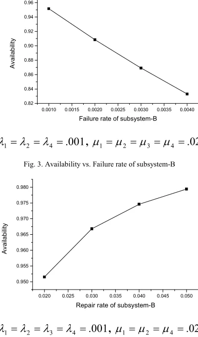
NALYSISThe effect of failure rates and repair rates of various components comprising the system is examined and it is found of failure rate (λ3) and repair rate (µ3) of the
subsystem-B highly affects the long run availability of the system. Their impact is shown in figures 3 & 4.
0.0010 0.0015 0.0020 0.0025 0.0030 0.0035 0.0040 0.82
0.84 0.86 0.88 0.90 0.92 0.94 0.96
A
v
a
ila
b
ili
ty
Failure rate of subsystem-B
001
.
4 2 1
=
λ
=
λ
=
[image:5.612.84.284.368.709.2]λ
,µ
1=
µ
2=
µ
3=
µ
4=
.
02
Fig. 3. Availability vs. Failure rate of subsystem-B
0.020 0.025 0.030 0.035 0.040 0.045 0.050 0.950
0.955 0.960 0.965 0.970 0.975 0.980
A
v
a
ila
b
ili
ty
Repair rate of subsystem-B
001
.
4 3 2
1
=
λ
=
λ
=
λ
=
λ
,µ
1=
µ
2=
µ
4=
.
02
Fig. 4. Availability vs. Repair rate of subsystem-B
VII
C
ONCLUSIONExpressions for mission reliability function, mission repairability and availability of spinning solution preparation system are derived. Determining mission reliability function is quite useful when quantifying workloads for repair facilities assuming that active repair time and total down time are approximately the same. The results of Process availability analysis highlight that the failure and repair rates of the subsystem-B (blend tank) highly affect the long run availability of the system. On failure of the blend tank the process availability will decrease by 4.85 percent if its repair will not be completed in the target time of four hours. Therefore it is recommended that a standby blend tank must be introduced in the existing system to run the system continuously without any interruption. This will also facilitate to avoid storage of high volume of buffer stock of spinning solution.
R
EFERENCES[1] Dyer D., “Unification of reliability/availability models for Marko systems” IEEE Transaction on reliability, Vol. 38, 1985.
[2] Kumar D., et all, ‘‘Availability of the feeding system in the sugar Industry’’, Micron reliability, 1988, Vol. 28, No. 6.
[3] R.T. Islamov, ‘‘Using Markov Reliability Modelling for Multiple Repairable Systems’’, Reliability engineering and system safety, 1994, pp. 113 - 118
[4] Microelsen Q., ‘‘Use of Reliability technology in the process industry’’, Reliability engineering and system safety, 1998, pp. 179 - 181
[5] Tsai Y., Wang K. and Tsai L., ‘‘A study of availability centered preventive maintenance for multi component system’’, Reliability Engineering and System Safety 84 (2004), pp. 261-270.
[6] Gupta P., Singh J., and Singh I.P., ‘‘Maintenance Planning based on Performance Analysis of 7-out-of-14: G Chemical-system: a Case Study,’’, International Journal of Industrial Engineering, 2005, pp. 264-274. [7] Shrama R.K. and Kumar S., ‘‘Performance modeling in
critical engineering systems using RAM analysis’’, Reliability Engineering and System Safety 93 (2008), pp. 891-897.
[8] Guo H., Watson S., Tavner P. and Xiang J.‘‘Reliability Analysis of Wind Turbines with incomplete failure data collected from after the date of initial installation’’, Reliability Engineering and System Safety 94 (2009), pp. 1057-1063.
Annexure-I
(8)
µ
4( )
x
µ
3( )
x
λ
3 (3)
λ
3λ
4µ3
( )
x µ4( )
x
µ
i( )
xλ
iµ
i( )
xλ
iµ
i( )
x(6)
λ
3λ
4µ3
( )
x µ4( )
x
λ
3−iµ
3−i( )
x
µ
3−i( )
x
(7)
µ
i( )
x
Working with Working at Failed full capacity reduced capacity state = if t ‹ τ = if t ‹ τ
= if t › τ = if t › τ
Fig. 2. State transition diagram (5)
φ
E
B
A
ir,,3g−i r2 , 1
=
i
(4)
o g r r
i
i B E
A,,3−
2 , 1
*=
j (2)
φ
E
B
A
iggi r, 3 , −
2 , 1
=
i
(0) o o o o
i
i B E
A , 3
,−
2 , 1
=
i
d o o o
i
i B E
A,,3−
i=1,2
d o o r
i
i B E
A , 3
,−
i=1,2
o o r o
i
i B E
A , 3 ,−
i=1,2
d r g g
i
i B E
A , 3 ,−
i=1,2
(1) o o o r
i
i B E
A,3,−
2 , 1
=