Online Full Text



Abstract—In order to decrease the chattering generated by

the sliding mode controller (SMC) in the manipulator trajectory tracking, we present a new adaptive sliding mode controller based on radial basis function (RBF) neural network.

The sliding mode variable structure control is used for resisting disturbance and guaranteeing the system stability, and the RBF neural network is introduced to reduce the switching gain through self-learning ability. The input of RBF neural network is the sliding mode function, and its output is the switching gain which can be adjusted adaptively. Under the condition of existing model errors and external disturbances, the simulation studies on the multi-joint rigid manipulator show that the proposed algorithm can obtain good performance both in tracking the trajectory and reducing the chattering.

Index Terms—manipulator, RBF neural network, sliding mode variable structure control, trajectory tracking

I. INTRODUCTION

he manipulator system is a time-varying, strong coupling and nonlinear system. The manipulator trajectory tracking have attracted considerable attentions of scholars [1]-[3].

Sliding-mode control is a robust design methodology using a systematic scheme based on a sliding surface and Lyapunov’s stability theorem. The main advantage of SMC is that the system uncertainties and external disturbances can be accommodated because of the invariance characteristics of system sliding conditions. However, the switching control in SMC results in control gain chattering. When the model of the manipulator is precisely known, Zhai et al. [4] proposed a new improved dual power reaching law based on the traditional sliding mode control. The adaptive items were added based on the dual power reaching law, the variables



and k were adjusted to effectively improve the approaching speed. The simulation result shows that the method has less chattering for the manipulator trajectory tracking. However, manipulator system is a complex nonlinear system, whose dynamic parameters are difficult to be forecasted precisely. In fact, it is almost impossible to obtain exact dynamic Manuscript received April 17, 2015; revised July 5, 2015. This work was supported in part by the key scientific research project of universities and colleges of Henan Province under Grant 15A413003.

Haitao Zhang is with the Information Engineering College, Henan University of Science and Technology, Luoyang, CO 471023 China (corresponding author: e-mail: [email protected]).

Mengmeng Du is with the Information Engineering College, Henan University of Science and Technology, Luoyang, CO 471023 China.

Wenshao Bu is with the Information Engineering College, Henan University of Science and Technology, Luoyang, CO 471023 China.

models because of such uncertainties as nonlinear frictions and flexibilities of the joints and links of manipulator. In the literature [5], the genetic algorithm was used to optimize the switching function, the size of the chattering as the index of fitness function was optimized, and a switching function with relative minimum chattering was constructed. Feiy et al. [6] presented a sliding mode control based on disturbance observer for robot, the coupling system was decoupled by the feedback joint angle; it achieved high precision, but the simple control structure demanded that the control parameters must be known. In literature [7], the sliding mode control was applied to deal with the robust control of space robot in capturing operation of the target and controlling the spacecraft motion under unknown parameters. The saturation function was introduced in order to avoid the chattering phenomena, the simulation results proved the feasibility of the algorithm.

The self-learning characteristics and high parallel computing characteristic of neural network are very powerful, it can approximate the nonlinear systems with arbitrary accuracy, and it also has a strong robustness. In addition, aiming at the approximation errors of the neural network, most of the researches get the result that the tracking errors can be uniformly ultimately bounded or can be kept arbitrarily small if some gain parameters are sufficiently large. Lin et al. [8] combined sliding mode control and RBF neural network to design the controller. The output of RBF neural network was regarded as the input of sliding mode controller. It achieved a certain effect on eliminating the chattering, but it used the objective function to estimate the network weights, so it can not realize the adaptive weight updated online. The controller of literature [9] was composed of SMC, RBF neural network, and fuzzy control. A Lyapunov function was selected for the design of the SMC, and RBF neural network was proposed to compute the equivalent control. The weights of the RBF neural network were adjusted according to an adaptive algorithm. Fuzzy logic was used to adjust the gain of the corrective control of the SMC. The real time implementations indicated that the proposed method can be applied to manipulator trajectory control. In this paper, the RBF neural network and sliding mode controller is designed serially, RBF neural network approximate the switching gain, and the robust term is used to eliminate the neural network error. The simulation results demonstrate that the chattering and the steady state errors are eliminated and satisfactory trajectory tracking is achieved.

The paper is organized as follows. In section 2, the related knowledge of the manipulator is introduced. In section 3, the slide model control method is described, and its disadvantages are discussed; the sliding mode controller with

Sliding Mode Controller with RBF Neural

Network for Manipulator Trajectory Tracking

Haitao Zhang, Mengmeng Du and Wenshao Bu

T

IAENG International Journal of Applied Mathematics, 45:4, IJAM_45_4_12

RBF neural network is designed and the stability proof is presented. Section 4 gives an example of a two degrees of freedom robot arm to show the effect of the proposed method. In Section 5 the concluding remarks are discussed.

II. PRELIMINARIES A. Model of Manipulator

A standard method for deriving the dynamics equations of a mechanical system is via the Euler-Lagrange equations. Using this method, the dynamics equations of a n degree of freedom rigid manipulator can be described in the following general form [10]:

( ) ( , ) ( ) _d

D q qC q q q G q 







(1)

WhereD q( ) is an n n inertia matrix, which is a positive

definite matrix. C q q( , ) is an n n matrix containing the centrifugal and Coriolis forces. G q( ) is an n1 vector containing gravity torques. qis joint position, q is joint velocity, q is joint acceleration.



is joint drive torque.



_d denotes the external disturbance and

0

T d ddt

 





is

bounded.

The dynamic characteristics of manipulator system are as follows:

Property 1: Inertia matrix D q( ) is a symmetric positive definite matrix bounded by ₁ 2 T ( ) ₂ 2

d x x D q xd x ,

where d₁and d₂ are known positive constants.

Property 2:The matrix D q( ) 2 ( , ) C q q is skew-symmetric, so it satisfies _{x D q x}T ( ) 2_{x C q q x}T ( , )_{ , x}_Rn_.

Property 3: The unknown disturbance satisfies



_{d } b_d,

where b_d is a positive constant.

Our objective is to design a trajectory tracking controller whose output is the control torque , which can make the position of joints track the desired trajectory accurately.

B. RBF Neural Network

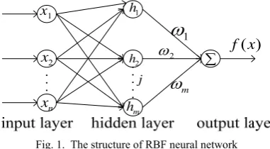
RBF neural network was proposed by J. Moody and C. Darken in the 1980s, and the corresponding theory was developed by Powell. It is a powerful feed forward neural network architecture [11]. This type of network was applied to the real multivariable interpolation problem and was first formulated as neural network by Broomhead and Lowe. In the control engineering, the RBF neural network is usually used as a tool for modeling nonlinear function up to a small error tolerance because of its good capabilities in function approximation.

The structure of typical RBF neural network is made up of a collection of parallel processing units called nodes as shown in Fig. 1:

2

x

n x

1 h

2

h

m

h

1



2



m



( ) f x  1

x

[image:2.595.330.521.54.159.2]

j

Fig. 1. The structure of RBF neural network

The RBF neural network has a feed forward architecture with an input layer, a hidden layer, and an output layer. The hidden layer is responsible for nonlinear transformation from the input space to the hidden space. The output layer is linear, which is designed to provide the response to the input signal. There is a layer of processing units called hidden units between the inputs and outputs. Each of them is implemented by a radial basis function. The input layer of the network has

n units for an n dimensional input vector. The input units are fully connected to the hidden layer units, which are in turn fully connected to the output layer units. In this paper, the number of input layer is 2, the number of hidden layer is 5, the number of output layer is 1.

The input-output mapping relationship is:

1

( ) m T ( )

j

f x  h x







(2)

Where x is the input signal of neural network, f x( )is the output signal, h x( )is the Gaussian basis function, and



denotes neural network weights.

The activation function of the hidden layer is generally a Gaussian function which is expressed as:

2 ₂

( ) e x p ( _j / _j )

h x   x c b ₍₃₎

Where

c

j are the RBF centers in the input vector space. j

b

denote the width of the node,

j



1, 2,



,

m

.

Under the condition of the following assumptions, RBF neural network can approximate continuous functions with any degree of accuracy in a compact set [12].

1. The neural network output f xˆ( , )



ˆ is continuous. 2. The ideal approximation of the neural network output

is ˆ( , )*

f x



, for a very small positive number



₀,which has: *

0 ˆ

max f x( ) f x( ,



) 



(4)

Where



* is an n n matrix, and denotes the best approximation of neural network weights.

Define the approximation error of ideal neural network, namely:

* ˆ

( ) ( , )

f x f x



 



(5)

IAENG International Journal of Applied Mathematics, 45:4, IJAM_45_4_12

By the approximation capability of RBF neural network, the modeling error  is bounded, we assume that it is



₀.

* 0

sup ( )

f x

f x

ˆ

( , )









(6)

Where:

* *

ˆ( , ) T ( )

f x







h x (7)

III. THE DESIGN OF THE CONTROLLER A. The Design of the Sliding Mode Controller

Sliding mode variable structure is a class of nonlinear control. The characteristic of this kind of control is that it has no fixed structure, and can change movement way according to the specific circumstances so as to achieve the presupposition state. Because the given trajectory has no association with the system state and the external disturbance, so the control system has strong robustness, and operation method of this control is simple.

The control objective is to drive the joint position q to the desired positionq_d. Define the tracking error:

d

e q q (8)

Define the sliding surface:

s e



e (9)

Where



diag[



₁ 



_i

 

_n], _i 0. Define the reference state [13]:

r d

q   q s q 



e (10)

r d

q   q s q 



e

     (11)

Assuming that there is no external interference



_d,we choose the control input



:

ˆ Ksgns

 

  (12)

ˆ ˆ

ˆ

ˆ Dq_r Cq_r G As



      (13)

Where Dˆ ,Cˆ ,Gˆ are the estimated values of D,

C

,G

respectively, and Kdiag K[ ₁₁K_iiK_nn]is a diagonal positive definite matrix in whichK_iiis a positive constant and

1

[ _{i n}]

Adiag a a a is also a diagonal positive definite matrix in whichis a_i a positive constant. sgn( ) is a sign function, it is given as follows:

1 , 0

sgn( ) 0 , 0

1 , 0

s

s s

s

 



_ 

 



(14)

Substituting Eq. (12) and (13) into Eq. (1), we can get:

( ) sgn

Ds CA s  f K s (15)

Where   f Dq_r Cq_r  G ,   D Dˆ D ,

ˆ

C C C

   ,   G Gˆ G.

Assuming that   f_i f_{i bound}, where f_{i bound} is the boundary of f_i , we choose K_iisuch that:

ii i bound

K  f (16)

Define the Lyapunov function candidate:

( ) / 2

T

Ls D q s (17)

Differentiating (17) and considering Eq. (12), (13) and (15), we get [13]:

1

/ 2

[ ( ) sgn( ) ]

[ sgn( )]

[ sgn( ) ]

[ ( sgn( ))]

0 T T T T

T T

n

T i i ii i i

T

L s Ds s Ds

s C A s f K s Cs s As f K s

s f K s s As s f K s s As s As



 

      

    

   

   

  



 _ 

(18)

The control law of (12) and (13) may be sensitive to uncertainties in the process of tracking and may lead to chattering. In addition, there is a difficulty to determine the switching gain of a sliding mode controller to achieve desired performance. At present, a trial and error procedure is commonly used to tune the parameters of the sliding mode controller. Thus the problem considered in our work is to propose a method to tune adaptively the switching gain K

of the SMC in order to achieve accurate and robust tracking of the manipulator with minimum chattering phenomena.

B. The Design of the RBF Neural Network Sliding Mode Controller (RBFNNSMC)

The design of the structure is shown as Fig. 2:

IAENG International Journal of Applied Mathematics, 45:4, IJAM_45_4_12

s s      

e

s e ce

 



e K  q q v  ˆ

D  Cˆ  Gˆ

e

e 

       d q  d

q qd



Fig. 2. The structure of trajectory tracking control with RBFNNSMC Manipulator equation is shown as Eq. (1), the new control law is as follows:

ˆ ˆ

ˆ

r r

Dq Cq G As K v



        (19)

Where K [ , ]k k_{1 2} is the output of RBF neural network of two joint manipulator; v is the robust term,

0

( _d)sgn( )

v



b s ， it is used for overcoming the neural network approximation error and external interference



_d.

Substituting Eq. (19) into Equation (1), yield:

( )

Ds CA s   f K v (20)

The adaptive law is designed as:

( )

i Ps h si i



  (21)

Where i1,2 represents the joint 1 and joint 2 of manipulator. Pis a symmetric positive definite matrix, and its inverse matrix is existing.

Let us introduce the candidate Lyapunov function:

2

1

1

/ 2 ( ) / 2

T T

i i i

L s Ds



P





 



  (22)

Where

* ˆ

i i i

  

   (23)

Differentiating (22), we get:

2 1 1 1 2 1 1 2 1 1 2 1 1 2 1 1

( ) / 2 ( ) / 2

(2 ) / 2 ( )

( ) ( )

[ ( ) ] ( )

( ) ( )

T T T T T

i i i i

i

T T T

i i i T T i i i T T i i i

T T T

i i i

L s Ds s Ds s Ds P P

s Ds s Ds P

s Ds Cs P

s C A s f K v Cs P

s As s f K P s

                                                 











   _  _{    }   _{ }            2 2 1 1 1 ( ) ( ) T

T T T

i i i i i

i i

v s As s f k  P s v

 

  



  



  

(24)

Because of T

( )

*T

( )

i i i i i

k







h s





h s

, we obtain:

2 2 * 1 1 1 2 2 * 1 1 1 2 2 * 1 1 1 ( ) ( ) ( ) ( ) ( ) ( )

T T T T T

i i i i i i

i i

T T T T T

i i i i i i i

i i

T T T T

i i i i i i

i i

L s As s f h h P s v

s As s f h s h P s v

s As s f h s h P s v























                               













  _{  }        (25)

Substituting Eq. (21) into Eq. (25), yield:

2

*

1

[ ( )]

T T T

i i i i i

L s As s f



h s s v



  



  

 ₍₂₆₎

The existence of a very small positive real number



_i, which makes the Eq. (26) satisfy:

*T _{( )}

i i i i i

f



h s

 

s

    ,0 



_i 1 (27)

Then :

2

*T _{( )} 2

i i i i i i i i

s  f



h s 



s 



s (28)

Therefore: 2 2 1 2 2 2 0 1 ( ) 0 T T i i i

i i i i d

i

L s As s s v

a s s s b







           





 (29)

Where



_idiag[ , ]

 

_{1 2} , a_i 



_i,



₀ 0, b_d 0. According to Eq. (29), only whens0, L0, the adaptive law asymptotic convergence. Finally, we may get the following conclusion:

lim lim( ) 0

tst e



e 

 (30)

IAENG International Journal of Applied Mathematics, 45:4, IJAM_45_4_12

Namely:

lim _d

tqq , limtqqd (31) From the above analysis it can be seen that the RBFNNSMC method can guarantee that the tracking errors converge arbitrarily close to zero. The following case study based on simulation will demonstrate this conclusion.

IV. SIMULATION RESULTS A. The Simulation of Two DOF manipulator

In this section, a simulation study is conducted to demonstrate the performance of our algorithm. A simple two degrees of freedom (DOF) manipulator is shown in Fig. 3. The dynamic equation is given as follows:

( ) ( , ) ( ) _d

D q qC q q q G q 







(32)

Where:

1 2 3 2 2 3 2

2 3 2 2

2 cos cos

( )

cos

p p p q p p q

D q

p p q p

  

 

  _ 

  (33)

3 2 2 3 1 2 2

3 1 2

sin ( )sin

( , )

sin 0

p q q p q q q

C q q

p q q

  

 

  

 

  



 (34)

4 1 5 1 2

5 1 2

cos cos( )

( )

cos( )

p g q p g q q

G q

p g q q

 

 

  _ 

  (35)

[0.2sin( ) 0.2sin( )]T

d t t



 (36)

1

1 r

2

0.87 r

1

q

2

m

2

q

1

[image:5.595.304.545.202.634.2]

m

Fig. 3. Structure of the manipulator

The mass of link 1 is m₁2.04kg, the mass of link 2 is

2 1

m  kg, the length of link 1 isr₁1m, and the length of link 2 is r₂0.87m. The 2

1 ( 1 2)1

p  m m r , 2

2 2 2

p m r ,

3 2 1 2

p m r r , p₄ (m₁m r₂)₁ , p₅m r_{2 2} , and

2 9.8 /

g m s .

The desired trajectory of the manipulator is q_1d 2sin( )t

andq_2d sin( )t , and the initial states of the manipulator are

1(0) 2(0) 0

q q 

,

q₁(0)q₂(0) 0

.

The RBF neural

network input is sliding mode function s and its differential

term s. The parameters of the Gaussian basis function are

100 50 0 50 100

5 0 5

10 10

c    _

 

 , b50.

The control parameters

{100,100} diag



 , Adiag{27,27} ,

{10,10,10,10,10}

Pdiag . In the robust term,



₀0.3,

0.2

d

b  . SIMULINK and S function is used to design the control system. In order to compare the advantages of the proposed method, under the same given parameters, we simulate the sliding mode control method and the proposed method. The simulation results are shown as Fig. 4-Fig. 12.

0 1 2 3 4 5 6 7 8 9 10

-2 0 2 4

Jo

in

t

1

(r

ad

)

SMC position tracking ideal position signal

0 1 2 3 4 5 6 7 8 9 10

-1 0 1 2

Time (s)

Jo

in

t 2

(

ra

d)

SMC position tracking ideal position signal

Fig. 4. Position tracking of SMC

0 1 2 3 4 5 6 7 8 9 10

-2 0 2 4

Joi

nt

1

(r

ad)

RBFNNSMC position tracking ideal position signal

0 1 2 3 4 5 6 7 8 9 10

-1 0 1 2

Time (s)

Joi

nt

2

(r

ad

)

RBFNNSMC position tracking ideal position signal

Fig. 5. Position tracking of RBFNNSMC

It can be seen from Fig. 4 and Fig. 5, the position tracking curves of joint 1 and 2 of manipulator are both ideal under the control of the two kind of algorithms.

IAENG International Journal of Applied Mathematics, 45:4, IJAM_45_4_12

[image:5.595.52.271.334.617.2]

0 1 2 3 4 5 6 7 8 9 10 -0.04

-0.02 0 0.02 0.04

time(s)

Jo

in

t 1

(

ra

d)

0 1 2 3 4 5 6 7 8 9 10

-0.02 0 0.02 0.04

0.01

-0.01

time(s)

Jo

in

t 2

(

ra

d)

Fig. 6. Position tracking error of SMC

0 1 2 3 4 5 6 7 8 9 10

-10 -5 0 5

2 x 10-3

Jo

int

1

(r

ad)

0 1 2 3 4 5 6 7 8 9 10

-0.02 -0.01 0 0.01 0.02

time(s)

Joi

nt

2

(r

[image:6.595.311.544.53.444.2]

ad)

Fig.7. Position tracking error of RBFNNSMC

Fig. 6 and Fig. 7 show the position tracking error of the two joints. Fig. 6 shows that the position tracking error under the control of SMC, the sdeady error of joint 1 fluctuates between 0.025 to -0.025, and the sdeady error of joint 2 fluctuates between 0.01 to -0.01. Fig. 7 shows that the position tracking error under the control of RBFNNSMC, the steady state error of joint 1 ranges from 0.002 to -0.006, the steady state error of joint 2 ranges from 0.01 to -0.01. From the error comparison of joint 1, we can know that the control precision of RBFNNSMC is better than SMC. As to the steady state error of joint 2, it is hard to compare the RBFNNSMC quantitatively with SMC, but the initial error under the control of RBFNNSMC is smaller than SMC. From Fig. 6 and 7 we can prove, the global performance of the system is improved using the RBF neural network, and because of using of the robust control term, the adverse effects which caused by the neural network approximation error is compensated effectively.

0 1 2 3 4 5 6 7 8 9 10

-2 0 2 4

Jo

in

t

(r

ad

/s)

SMC velocity tracking ideal velocity signal

0 1 2 3 4 5 6 7 8 9 10

-2 0 2 4

Time (s)

Jo

in

t 2

(

ra

d/s

)

SMC velocity tracking ideal velocity signal

Fig. 8. Velocity tracking of SMC

0 1 2 3 4 5 6 7 8 9 10

-2 0 2 4

Jo

in

t

(r

ad

/s)

RBFNNSMC velocity tracking ideal velocity signal

0 1 2 3 4 5 6 7 8 9 10

-1 0 1 2

Time (s)

Jo

in

t 2

(

ra

d/

s)

RBFNNSMC velocity tracking ideal velocity signal

Fig. 9. Velocity tracking of RBFNNSMC

From Fig. 8 and Fig. 9, we can conclude that the velocity tracking errors have big fluctuation under the control of SMC. However, the velocity curve under the control of RBFNNSMC can trace the given velocity signal smoothly.

0 1 2 3 4 5 6 7 8 9 10

-200 0 200 400 600

time(s)

C

on

tr

ol

in

pu

t 1

(

N

m

)

0 1 2 3 4 5 6 7 8 9 10

-400 -200 0 200 400

time(s)

C

ont

rol

in

pu

t

2

(N

m

[image:6.595.51.289.54.449.2]

)

Fig. 10. Control torque of SMC

IAENG International Journal of Applied Mathematics, 45:4, IJAM_45_4_12

[image:6.595.307.548.509.702.2]

0 1 2 3 4 5 6 7 8 9 10 -200

0 200 400 600

time(s)

C

on

tr

ol

in

pu

t 1

(

N

m

)

0 1 2 3 4 5 6 7 8 9 10

-50 0 50 100 150 200

time(s)

C

on

tr

ol

in

pu

t 2

(

N

m

[image:7.595.51.287.52.244.2]

)

Fig. 11. Control torque of RBFNNSMC

Fig. 10 and Fig. 11 show the output control torque of manipulator, Fig. 10 shows the chattering of SMC is very big, so this control method is very difficult to apply in practice. After joining the RBF neural network controller, the system can adaptively adjust the switching gain, which reduces the system chattering caused by sliding mode control.

0 2 4 6 8 10

0 1 2 3

time(s)

K

1

0 2 4 6 8 10

0 0.5 1 1.5 2

time(s)

K

[image:7.595.356.488.60.187.2]

2

Fig. 12. The adaptive change of gain under the RBFNNSMC Fig. 12 shows the changing process of switching gain under the adjustment of the RBF neural network.

B. The Simulation of Three DOF manipulator

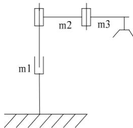
In order to verify the effectiveness of the algorithm, we use the assembly manipulator in the literature [14] to do the simulation. It is a space manipulator with three degrees of freedom. The diagram is shown in Fig. 13, the first joint do the translational motion, the second joint and the third joint do the revolving motion.

Fig.13. The diagram of the three DOF manipulator

We can know the parameters from the literature [14], the mass of link 1 is m₁1kg, the mass of link 2 is m₂ 1kg, the mass of link 3 is m₃1kg

,

the length of link 2 is

1 0.2

l  m, and the length of link 3 is l₂0.2m. Dynamic matrices are shown below:

11

22 23

32 33

0 0

( ) 0

0 a

D q a a

a a

 

 

  

 

 

(37)

22 23

32

0 0 0

( , ) 0

0 0

C q q b b

b

 

 

  

 

 

 (38)

1 2 3

( )

( ) 0

0

m m m g

G q

 

 

 

  

 

 

(39)

Where

11 1 2 3

a m m m (40)

2 2 2

22 2 2 / 3 3 3 / 3 3 2 2 3 3cos( )3

a m l m l m l l l m q (41)

2

23 32 3 3 / 3 2 3cos( )3 3/ 2

a a m l l l q m (42)

22 2 3sin( )3 3 3/ 2

b  l l q m q (43)

23 3 2 3sin( ) / 23 3 3 2 3sin( )3 2/ 2

b  m l l q q m l l q q (44)

32 3 2 3sin( )3 2/ 2

b  m l l q q (45)

The desired trajectory of the manipulator is q_1d 2sin( )t ,

2d sin( )

q  t , q_3d sin(2 )t , and the initial states of the manipulator are q₁(0)q₂(0)q₃(0) 0 ,

1(0) 2(0) 3(0) 0

q q q  . External disturbance is

[0.2sin( ) 0.2sin( ) 0.1sin( ) ]T

d t t t



 . The RBF neural

network parameters are

10 10 10 10 10 1 1 1 1 1 5 5 5 5 5 c

 

 

  

 

 

and b5.

The inputs are the sliding mode function of the three joints respectively, namely, s(1), s(2)and s(3). The structure of the RBF neural network is 3-5-1. The control parameters

{80,80} diag



 , A diag {30,30} and

IAENG International Journal of Applied Mathematics, 45:4, IJAM_45_4_12

[image:7.595.308.547.217.593.2] [image:7.595.51.290.337.531.2]

{10,10,10,10,10}

Pdiag . In the robust term,



₀0.3,

0.2

d

b  . The simulation results are shown as Fig. 14-Fig. 18 .

0 0.5 1 1.5 2 2.5 3 3.5 4 4.5 5

-2 0 2 4

Jo

in

t 1

(

ra

d) RBFNNSMC position tracking

ideal signal

0 0.5 1 1.5 2 2.5 3 3.5 4 4.5 5

-1 0 1 2 3

Jo

in

t 2

(

ra

d) RBFNNSMC position tracking

ideal signal

0 0.5 1 1.5 2 2.5 3 3.5 4 4.5 5

-1 0 1 2 3

Jo

in

t 3

(

ra

d) RBFNNSMC position tracking

[image:8.595.50.284.56.489.2]

ideal signal

Fig. 14. Position tracking of RBFNNSMC

0 0.5 1 1.5 2 2.5 3 3.5 4 4.5 5

-0.02 -0.01 0 0.01

P

os

iti

on

E

rr

or

(

rad) _{Joint 1}

0 0.5 1 1.5 2 2.5 3 3.5 4 4.5 5

-4 -2 0 2 4

x 10-3

P

os

iti

on

E

rro

r

(rad

)

Joint 2

0 0.5 1 1.5 2 2.5 3 3.5 4 4.5 5

-2 0 2x 10

-3

Time (s)

P

os

iti

on

E

rror

(r

ad

)

Joint 3

Fig.15. Position tracking error of RBFNNSMC

We can conclude from the Fig. 14 that tracking curves of the three joints are very ideal. Fig. 15 are the position error curves of three joints. The tracking error of joint 1 is 0.002; the tracking error of the joint 2 and joint 3 is also very small, it is 10-3 _{order of magnitude.}

0 0.5 1 1.5 2 2.5 3 3.5 4 4.5 5

0 0.005 0.01

K

1

0 0.5 1 1.5 2 2.5 3 3.5 4 4.5 5

0 2 4x 10

-3

K 2

0 0.5 1 1.5 2 2.5 3 3.5 4 4.5 5

0 2 4x 10

-3

Time (s)

K

[image:8.595.307.544.88.491.2]

3

Fig. 16. The adaptive change of gain under the RBFNNSMC

Fig. 16 is the changing process of switching gain under the adjustment of the RBF neural network.

0 0.5 1 1.5 2 2.5 3 3.5 4 4.5 5

-100 0 100 200 300

Jo

in

t1

T

orque

(

Nm

)

0 0.5 1 1.5 2 2.5 3 3.5 4 4.5 5

-10 0 10

Jo

in

t2

T

orque

(

Nm

)

0 0.5 1 1.5 2 2.5 3 3.5 4 4.5 5

-5 0 5

Time (s)

Jo

in

t3

T

or

qu

e (

N

m

)

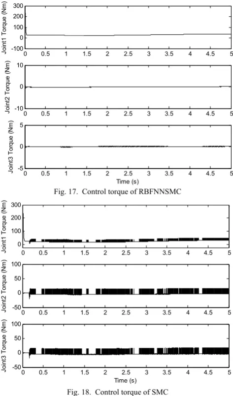
Fig. 17. Control torque of RBFNNSMC

0 0.5 1 1.5 2 2.5 3 3.5 4 4.5 5

0 100 200 300

Jo

in

t1

T

or

que

(N

m

)

0 0.5 1 1.5 2 2.5 3 3.5 4 4.5 5

-50 0 50 100

Joi

nt

2

T

or

qu

e

(N

m

)

0 0.5 1 1.5 2 2.5 3 3.5 4 4.5 5

-50 0 50 100

Time (s)

Jo

in

t3

T

or

qu

e (

N

m

)

Fig. 18. Control torque of SMC

Fig. 17 is the output torque under the control of RBFNNSMC. Fig. 18 is the output torque under the control of traditional SMC. Because of the gravity term of joint 2 and joint 3 are zero, so the output torques are very small in the Fig. 17 and Fig. 18. We can see that the chattering is very big under the control of traditional SMC. However, there is almost no chattering under the control of RBFNNSMC.

V. CONCLUSION

This paper mainly studies the multi-joint manipulator system with uncertainties for the trajectory tracking control. This paper combines the sliding mode control with RBF neural network. The sliding mode control is used to resist interference and ensure the stability of the system, RBF neural network is used to adjust the sliding mode gain online, so as to reduce the chattering of output torque. The RBF neural network approximation error is overcome by adding the robust term. The design guarantees the closed-loop stability by using Lyapunov method. The simulation results show that the proposed control method is appropriate for design of manipulator with uncertainty and the external interference.

IAENG International Journal of Applied Mathematics, 45:4, IJAM_45_4_12

[image:8.595.51.290.570.758.2]

REFERENCES

[1] M. Rasheedat, Mahamood, “Improving the Performance of Adaptive PDPID Control of Two-Link Flexible Robotic Manipulator with ILC,” Engineering Letters, vol. 20, no. 3, pp. 259-270, 2012.

[2] J. S. Kong, E. H. Lee, B. H. Lee and J. G. Kim, “ Study on the real- time walking control of a humanoid robot using fuzzy algorithm,” International Journal of Control, Automation and Systems, vol. 6, no. 4, pp. 551-558, 2008.

[3] P. K. Vempaty, K. C. Cheok, R. N. K. Loh, and S. Hasan, “Model Reference Adaptive Control of Biped Robot Actuators for Mimicking Human Gait,” Engineering Letters, vol. 18, no. 2, pp. 165-174, 2010. [4] W. N. Zhai，Y. W. Ge and S. Z. Song, “Sliding Mode Control for

Robotic Manipulators Based on the Improved Reaching Law,” Information and Control, vol. 43, no. 3, pp. 300-305, 2014.

[5] C. F, Wang Y N, He J, Long Y H, “GA-NN-integrated sliding-mode control system and its application in the printing press,” Control Theory and Applications, vol. 20, no. 2, pp. 217-222, 2003.

[6] N. FEIY, J. S. SMITH and Q. H. Wu, “Sliding mode control of robot manipulators based on sliding mode perturbation observation,” Systems and Control Engineering, vol. 220, no. 1, pp. 201-210, 2006. [7] T. Kobayashi and S. Tsuda, “Sliding Mode Control of Space Robot for

Unknown Target Capturing,” vol. 19, no. 2, pp. 105-111, 2011. [8] L. Lin, H. B. Ren and H. R. Wang, “RBFNN-based Sliding Mode

Control for Robot,” Control engineering of China, vol. 14, no. 2, pp. 224-226, 2007.

[9] A. Gokhan Ak, G. Cansever and A, Delibai, “Trajectory tracking control of an industrial robot manipulator using fuzzy SMC with RBFNN,” Gazi University Journal of Science, vol. 28, no. 1, pp. 141-148, 2015.

[10] M. Tan, D. Xu, Z. G. Hou, S. Wang and Z. Q. Cao. Advanced robot control. Beijing: Higher Education Press, 2007, pp. 452-454. [11] Y. S. Yang and X. F. Wang, “Adaptive H tracking control for a

class of uncertain nonlinear systems using radial-basis-function neural networks,” Neurocomputing, vol. 70, no. 4, pp. 935-941, .2007. [12] H. R. Wang, C. N. Liu and Y. X. Zhang, “A neural network robust

control based on the dissipative theory for robot,”. Control Engineering China, vol. 17, no. 6, pp. 853-855, 2010.

[13] J. K. Liu. Design and Matlab simulation of robotic control systems. Beijing, Qinghua university press, 2008

[14] Q. Liu. Research and application of error analysis and compensation methods of assembling manipulator. Zhenjiang, Jiangsu University, 2014.

IAENG International Journal of Applied Mathematics, 45:4, IJAM_45_4_12