Abstract—In this paper, a neural network-based sliding-mode controller design approach with decoupled method is proposed for a class of nonlinear discrete-time uncertain multi-input- multi-output (MIMO) systems. The neural network is used to generate the proper control inputs by simultaneous perturbation stochastic approximation (SPSA) algorithm. The decoupled method simplifies the design complexity to achieve asymptotic stability for the uncertain nonlinear system with external disturbance. The proposed control scheme does not need the exactly system model to avoid the mathematical derivation. In addition, the frictional force analysis for the nonlinear inverted double pendulum system is considered to investigate the relationship between controller and frictional force. Simulation results are presented to illustrate the effectiveness of our approach.
Index Terms—nonlinear control, neural network system,
decouple, sliding mode control, simultaneous perturbation stochastic approximation
I. INTRODUCTION
Sliding-Mode control (SMC) has been suggested as an approach for the control of systems with nonlinearities, uncertain dynamics and bounded input disturbances [1, 2]. SMC technique provides fast error convergence and strong robustness for control system [4, 5]. However, SMC requires system dynamic model of the plant and bounds on modeling uncertainty to formulate control laws with guaranteed stability. For solving this problem, the intelligent controllers, developed by principles of fuzzy logic, neural network (NN), and genetic algorithms, should be designed to achieve the control objective [1-5,7].
Recently, NN-based stable and on-line adaptive control has been paid much attention in nonlinear adaptive control [1, 3, 4, 7]. To develop the neural-network-based controller, the corresponding adaptive laws should be derived by the measurement of objective function. The usual used methods are gradient method and Lyapunov approach. However, it is difficult or impossible to directly obtain the gradient of objective function or the derivation of adaptive laws based on Lyapunov approach is difficult and complex to obtain. Therefore, stochastic approximation algorithms such as Kiefer-Wolfowitz finite difference gradient approximation and simultaneous perturbation stochastic approximation (SPSA) were proposed to solve these problems [13-15]. By using SPSA, we can only measure the objective function to solve the optimization problem for providing the adaptive
This work was supported in part by the National Science Council, Taiwan, R.O.C., under contracts NSC-99-2221-E-155-033-MY3.
Ching-Hung Lee is with Department of Electrical Engineering, Yuan-Ze University, Chung-li, Taoyuan 320, Taiwan. (phone: +886-3-4638800, ext: 7119; fax: +886-3-4639355, e-mail: [email protected]).
laws of NN.
In this paper, we propose a new neural-network-based decoupled sliding-mode controller scheme to solve the control of a class of multi-input-multi-output (MIMO) nonlinear dynamic systems via the SPSA algorithm. The considered nonlinear system has uncertainty, variant parameters, and external disturbance. We use the decoupled architecture and sliding-mode control approach for the input variables of NN system for simplifying the computational complexity. The weights of the NN are updated according to the results of SPSA algorithm for the purpose of controlling the system states to stay in sliding surface. The NN controller generates the proper control signal for the unknown nonlinear dynamic system. Through SPSA laws, we can adjust the parameters to achieve the stability objective. Finally, the frictional force analysis for the nonlinear inverted double pendulum system is considered to investigate the relationship between controller and frictional force. Simulation results are presented to illustrate the effectiveness of our approach.
This paper is organized as follows. Section II introduces the problem formulation and used neural network. The proposed new neural-network-based decoupled sliding-mode controller scheme (DSMCNN) is introduced in Section III. Section IV shows the simulation results. Conclusion is given in Section V.
II. PRELIMINARIES
A. System description
It is known that the coupling phenomenon is existed in many real-world systems. The so-called couple phenomenon is that a control force will influence the states simultaneous. Consider the ith sub-system of discrete-time nonlinear system represented by the following model
[
]
[
]
⎪ ⎪ ⎪
⎩ ⎪ ⎪ ⎪
⎨ ⎧
⋅ + ⋅ +
+ =
+ = + ⋅
+ + ⋅ + ⋅
+ =
+ = + ⋅
+
Ω
s i i i i
i i i
i
s i i i
s i i i i
i i i
i
s i i i
i
T k d k u k x g
k x f k x k x
T k x k x k
x g x k u k d k T
k x f k x k x
T k x k x k x
) ( ) ( )) ( (
)) ( ( ) ( ) 1 (
) ( ) ( ) 1 (
) ( ) ( )) ( (
)) ( ( ) ( ) 1 (
) ( ) ( ) 1 (
:
2 2
2 4
4
4 3 3
1 1
1 2
2
2 1 1
(1)
where i=1,.., n, xi(k)=[xi1(k) xi2(k) xi3(k) xi4(k)]T is the measurable state vector, fi1(x) and gi1(x),where i=1,..n, are
nonlinear discrete-time functions, ui is the control inputs, and
di1(t), di2(t), i=1,..n, are external bounded disturbances, i.e.,
|di1(t)|≤Di1,|di2(t)|≤Di2, i=1,... n. For this ith sub-system, our
control objective is to design the input ui such that state
vector xi converges to zero. Obviously, the decoupling
method should be adopted to decouple the state xi2 and xi4.
Neural Network-based Decoupled Sliding Mode
Controller Design for Discrete-time Nonlinear
MIMO Systems by SPSA Algorithm
Thus we utilize the method of literature [4, 5, 12] to design decoupled control in the discrete-time form.
For sub-system (1), we first define the following sliding surfaces
) 1 ( )) 1 ( ( ) 1 (
) 1 ( )) 1 ( ) 1 ( ( ) 1 (
4 3
2 2
2 1
1 1
+ + + =
+
+ + + − + =
+
k x k
x c k s
k x k z k x c k s
i i
i i
i i
i i i
(2) where zi(k+1)=−zUisat(si2(k+1)/φi2), with 0<zUi,<1, (sat(⋅) denotes the saturation function).
In the design of decoupled sliding-mode controller, we can give an equivalent control such that the states can stay on sliding surface. The equivalent control can be obtained by setting si1 are equal to zero. From equation (2), we can
observe that if si1 achieves to zero, then xi1 is equal to zi and xi2
also achieves to zero. We also find that zi and xi1 achieve to
zero simultaneously when si2 achieves to zero. Therefore, if
we derive si1 toward to zero, the control objective can be
achieved. In addition, the selection of coefficients ci1 and ci2
will affect the behavior in the transient state of the system. For achieving favorable transient response, proper choice of sliding factor is necessary.
According the above discussion, si1 will be fed into the
neural-network (NN) to generate the proper control signals. In addition, our control objective can also be transferred as to derive si1 to approach to zero.
Layer 3
Layer 2
Layer 1
11
s sn1
1 y
∑
j
1
ω
11
ω
∑
p
y
pj
ω 1 p ω
nj
v j
v1 11 v
1 i v
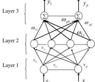
Figure1: Network diagram of the used NN system.
[image:2.595.313.539.220.372.2]B.NEURAL-NETWORK SYSTEM
Fig. 1 shows the schematic diagram of a three layer NN system. Layer 1 accepts input variables. Its nodes represent input linguistic variables. The nodes only transmit input variables to the next layer directly,
( )
k s( )
kOj i1
) 1
( = (3) where si1(k) is input at discrete-time index k. Layer2 is a
hidden layer.
( )
=∑
( ) ( )
⋅i
i ij
j k v k s k
net 1
) 2 (
(4)
( ) 2
) 2 (
) 1
( 1 )
( net(1)k
j k e j
O −
+
= (5) where vij(k) is the weight between the layer 1 and layer 2. Finally, Layer 3 is the output layer. The links between layer 2 and layer 3 are connected by weighting value
( )
∑
( ) ( )
=
= R
j
j pj
p k kO k
O
1
) 2 ( )
3
( ω
. (6)
III. DESIGN OF DECOUPLED NN SLIDING-MODE CONTROLLER
Most of control systems contain the un-model uncertainty, parameters variation, or external disturbance. Therefore, the
adaptive property and robustness analysis should be considered. In this section, we introduce the decoupled neural network sliding-mode controller for obtaining the equivalent control. This approach does not need the system dynamics model exactly. It uses the model free concept to develop the adaptive DSMCNN control scheme. Fig. 2 shows the decoupled adaptive control scheme. First, the system state variables are transferred into SMC variables s11
and s21 by the decoupled method (shown in equations (2)).
Then, the NN can generate the proper control signals such that the system outputs approach to zero. The adaptive laws of NN’s parameters can be derived by the following description.
xi(k+1)
SPSA Algorithm
Dynamic
System
0 0
x11(k)
x12(k)
x14(k)
x13(k)
u1(k)
u2(k)
+ +
-z1(k)
z2(k)
Neural
Network
s11(k)
s11(k)
s21(k)
s21(k)
sn1(k)
sn2(k)
xn2(k)
xn3(k)
xn4(k)
xn1(k)
0
+
-sn1(k)
sn1(k) )
(
21k
s
) (k zn
) (
22k
s
) (
11k
s
) (
12k
s
x21(k)
x22(k)
x24(k)
x23(k)
Figure 2:The proposed DSMCNN control scheme via SPSA. Our control goal is to minimize the following cost function:
∑
=
= n
i
i k
s k
E
1
2 1( )) ( 2 1 )
( (7) By the gradient-descent method, the update laws of NN’s parameters are
⎟ ⎟ ⎠ ⎞ ⎜
⎜ ⎝ ⎛
∂ ∂ − + =
Δ + =
+
pj pj
pj pj
pj
w k E η k w k w k w k
w ( 1) ( ) ( ) ( ) ( ) (8)
⎟ ⎟ ⎠ ⎞ ⎜
⎜ ⎝ ⎛
∂ ∂ − + = Δ + = +
ij ij
ij ij
ij
v k E η k v k v k v k
v ( 1) ( ) ( ) ( ) ( ) . (9)
To avoid deriving the gradient of objective function, we here utilize the SPSA algorithm to approximate
)
( ) (
)) ( ( )) ( ) ( ) ( ( ) (
k k R
k w E k k R k w E w
k E
pj pj
pj pj
pj pj
pj ⋅Δ
− Δ ⋅ + =
∂ ∂
(10)
) ( ) (
)) ( ( )) ( ) ( ) ( ( ) (
k k R
k v E k k R k v E v
k E
ij ij
ij ij
ij ij
ij ⋅Δ
− Δ ⋅ + =
∂ ∂
(11) where Rij(k) is perturbation due to the equation and Δij(k) is a
vector whose elements are either 1 or -1 in random.
Therefore, we should calculate, E(wpj(k)+Rpj(k)⋅Δpj(k)),
E(wpj(k)), E(vij(k)+Rij(k)⋅Δij(k)), and E(vij(k)) at first.
However, in experimental applications, we cannot feed two control forces to evaluate the corresponding objective values at the same time. In this paper, we use mathematics derivation to improve the problem.
From equation (7), we have
pj i i
pj w
k s k s w E(k)
∂ ∂ ⋅ = ∂
∂ ( )
)
( 1
[image:2.595.91.247.347.481.2]ij i i ij v k s k s v E(k) ∂ ∂ ⋅ = ∂ ∂ ( ) ) ( 1
1 . (13) Next, we use modified SPSA to approximate
pj i w k s ∂
∂ 1( )
. Substitute system (1) into the sliding surface (2), we have
[
( ( )) ( ( )) ( ) ( )]
). ) ( )) 1 ( ) ( ) ( ( ) 1 ( 1 1 1 2 2 1 1 1 s i i i i i i i i s i i i i T k d k u k x g k x f k x k z T k x k x c k s ⋅ + ⋅ + + + + − ⋅ + = + (14) The perturbed results is shown below:[
( ( )) ( ( )) ( ) ( )]
). ) ( )) 1 ( ) ( ) ( ( ) 1 ( 1 1 1 2 2 1 1 1 s i i i i i i i i s i i i i T k d k u k x g k x f k x k z T k x k x c k s ⋅ + ⋅ + + + + − ⋅ + = + Δ Δ (15) Using the SPSA algorithm to approximatepj i w k s ∂
∂ 1( )
, we obtain ) )) ( ( ( ) ( ) ( ) ( ) ( ) ( ) ( ) 1 ( ) 1 ( ) ( ) ( )) ( ( )) ( ) ( ) ( ( ) ( 1 1 1 1 1 1 s i i pj pj i i pj pj i i pj pj pj i pj pj pj i pj i T k x g k k R k u k u k k R k s k s k k R k w s k k R k w s k s ⋅ ⋅ Δ ⋅ − = Δ ⋅ + − + = Δ ⋅ − Δ ⋅ + = ∂ ∂ Δ Δ ω (16)
∑
= Δ ⋅ ⋅Δ ⋅ − = Δ ⋅ − Δ ⋅ + = ∂ ∂ n i s i i ij ij i i ij ij ij i ij ij ij i ij i T k x g k k R k u k u k k R k v s k k R k v s v k s 1 1 1 1 1 ). )) ( ( ( ) ( ) ( ) ( ) ( ) ( ) ( )) ( ( )) ( ) ( ) ( ( ) ( (17)
Substituting equations (16) and (17) into equations (12) and (13), we can obtain
). )) ( ( ( ) ( ) ( ) ( ) ( ) ( ) ( 1
1 i i s
pj pj i i i pj T k x g k k R k u k u k s k
E ⋅ ⋅
Δ ⋅ − ⋅ = ∂ ∂ Δ ω (18) ). )) ( ( ( ) ( ) ( ) ( ) ( ) ( ) ( 1
1 i i s
ij ij i i i ij T k x g k k R k u k u k s v k
E ⋅ ⋅
Δ ⋅ − ⋅ = ∂ ∂ Δ (19) Without derivation from the system dynamics model, we should evaluate the objective function twice for obtaining the gradient terms
pj i w k s ∂
∂ 1( )
and ij i v k s ∂
∂ 1( )
[image:3.595.80.256.632.746.2]. As above, we can obtain the same result without repetition evaluations. In addition, the control signal is proportional to the difference between the control input and perturbed control one. That is, the control input does not feed into the nonlinear system for evaluating the objective function. This provides a simple approach for real-time control system. In this paper, this approach is applied on a double pendulum on cars.
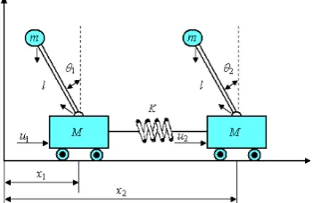
Fig. 3: System diagram of two inverted pendulums connected by a moving spring mounted on two carts.
IV. SIMULATION RESULTS
Herein, we apply the proposed approach to solve the stabilization of the two inverted pendulums connected by a moving spring mounted on two carts which is modified from [19].Fig. 3 is the diagram of inverted double pendulums on cars systems which includes the cars which can move horizontally and each car has a pendulum which swings left and right. In addition, these two cars are connected by a spring. In the diagram, u1 and u2 are control input forces of
the cars, X=[x1 x2]T is the output position of the car, θ=[θ1 θ2]T
is the angle between vertical axis and pendulum, and k is the spring constant, m is mass of load, M is mass of car, l is length of pendulum, r is the radius of load, and ml is mass of
pendulum, and L is the initial distance of two cars. In this paper, we consider the stabilization of X and θ, this is different from the previous literature.
For the further analysis of the dynamic system characteristic, we have to establish the mathematical model. Then we have the following motion equations.
)
( 2 1
1 1 1
1x u H K x x L
M && = − + − − )
( 2 1 2
2 2
2x u H K x x L
M && = − − − − (20)
where H denotes the pendulums’ horizontal forces 1 1 1 1 1 2 1 1 1 1 1
1 mx&& ml(θ& )sinθ mlθ&&cosθ
H = + −
2 2 2 2 2 2 2 2 2 2 2
2 m x&& ml (θ& )sinθ mlθ&&cosθ
H = + − (21)
The rotating motion equations for pendulums are
1 2 1 1 2 1 1 2 1 2 1 1 1 1 1 1 1 ) ) ( 5 2 3 1 ( ) cos sin ( θ θ θ && ⋅ + ⋅ + + + = ⋅ + r l m r m m m l m l H V L l 2 2 2 2 2 2 2 2 2 2 2 2 2 2 2 2 2 ) ) ( 5 2 3 1 ( ) cos sin ( θ θ θ && ⋅ + ⋅ + + + = ⋅ + r l m r m l m l m l H V L L (22) where 2 2 2 2 2 2 2 2 2 2 2 1 2 1 1 1 1 1 1 1 1 1 cos sin cos sin θ θ θ θ θ θ θ θ & && & && l m l m g m V l m l m g m V − − = − − = (23) Herein, we select m=m1=m2, M=M1=M2, and r=r1=r2 for
simplifying the design. Define the state variables as q11=θ1,
q12=θ&1, q13= x1, q14=x&1, q21= θ2, q22=θ&2, q23=x2-x1-L, and 1
2 24 x x
q = & −& . Therefore, system (20) can be represented as
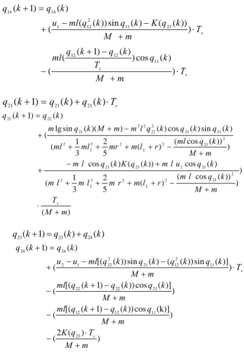
s T k q k q k
q11( +1)= 11( )+ 12( )⋅
) ( ) ) )) ( cos ( ) ( 5 2 3 1 ( ) ( cos )) ( ( ) ( cos ) )) ( cos ( ) ( 5 2 3 1 ( ) ( sin ) ( cos ) ( ) )( ( sin ( ) ( ) 1 ( 2 11 2 2 2 2 11 1 23 11 2 11 2 2 2 2 11 11 2 12 2 2 11 12 12 m M T m M k q ml r l m mr ml ml k q mlu k q K k q ml m M k q ml r l m mr ml ml k q k q k q l m m M k q mlg k q k q s L L L L + ⋅ + − + + + + + + + − + + + + − + + = + s T k q k q k
s s s T m M k q T k q k q ml T m M k q K k q k q ml u k q k q ⋅ + − + − ⋅ + − − + = + ) ) ( cos ) ) ( ) 1 ( ( ( ) )) ( ( ) ( sin )) ( ( ( ) ( ) 1 ( 11 12 12 23 11 2 12 1 14 14 s T k q k q k
q21( +1)= 21( )+ 21( )⋅
) ( ) ) )) ( cos ( ) ( 5 2 3 1 ( ) ( cos )) ( ( ) ( cos ) )) ( cos ( ) ( 5 2 3 1 ( ) ( sin ) ( cos ) ( ) )( ( sin lg ( ) ( ) 1 ( 2 21 2 2 2 2 21 2 23 21 2 21 2 2 2 2 21 21 2 22 2 2 21 22 22 m M T m M k q l m r l m r m l m l m k q u l m k q K k q l m m M k q ml r l m mr ml ml k q k q k q l m m M k q m k q k q s L L L L + ⋅ + − + + + + + − + + − + + + + − + + = + ) ( ) ( ) 1
( 23 24
23 k q k q k
q + = +
) ) ( 2 ( ) (k)] cos )) ( ) 1 ( [( ( ) )] ( cos )) ( ) 1 ( [( ( ) )] ( sin )) ( ( ) ( sin )) ( [( ( ) ( ) 1 ( 23 11 12 12 21 22 22 11 2 12 21 2 22 1 2 24 24 m M T q K m M q k q k q ml m M k q k q k q ml T m M k q k q k q k q ml u u k q k q s s + ⋅ − + − + − + − + − ⋅ + − − − + = + (24) According the decoupled control scheme introduced above, we define ) 1 ( ) 1 ( ) 1 ( ) 1 ( )) 1 ( ) 1 ( ( ) 1 ( ) 1 ( ) 1 ( ) 1 ( ) 1 ( )) 1 ( ) 1 ( ( ) 1 ( 24 23 22 22 22 2 21 21 21 14 13 12 12 12 1 11 11 11 + + + = + + + + − + = + + + + = + + + + − + = + k q k q c k s k q k z k q c k s k q k q c k s k q k z k q c k s (25) where 1 0 ), / ) ( ( ) ( 1 0 ), / ) ( ( ) ( 2 4 22 2 2 1 2 12 1 1 < < − = < < − = U U U U z k s sat z k z z k s sat z k z φ φ
In the simulation, the following specifications are used: g=9.8m/s2
, l=0.5m, ma=0.8kg, m=0.1kg, r=0.01m, L=0.1m,
k=1, c1=5, c2=0.5, Φ1=5, Φ2=15, zU1=π/4, c3=5, c4=0.5, Φ3=5,
Φ4=15, zU2=π/4. Initial condition is [-π/12, 0, -π/12, 0, 0, 0,
0.1, 0]. The sample time Ts is 0.002 second. The
corresponding learning rates for NN are ηw=0.3/T
[image:4.595.46.289.49.399.2]s, ηv=0.1/Ts.
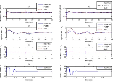
Fig. 4 and 5 show the simulation results of system without disturbance and perturbed by impulse, respectively. According to the simulation result of Fig. 4, we can find that the decoupled NN controller and SMC are better than the results of using fuzzy logic control approach. From the comparison results of performance in stabilizing time, we can find that DSMCNN control has the better performance.
Subsequently, we discuss the effect if there are external disturbance. Firstly, when the simulation time T=15sec, we add external disturbance such as θ1=-π/20. Fig. 5 shows the
simulation results. After adding disturbance, we could obviously find that the disturbance rejection ability of NN performed better than fuzzy logic control and SMC. For the consideration of robustness, we can find that NN only need
smaller effort such that system outputs achieve to stable even system having external disturbance.
In addition, we consider the effect of frictional force. In real system, the frictional force may result in a delay appearance. In the system model, we use the frictional force model as the following description [6]. After considering the frictional force, the horizontal displacement should be
3 1 2 1 1 1
1x u H k(x x L) F
M && = − + − − −
4 1 2 2 2 2
2x u H k(x x L) F
M && = − − − − − (26)
The inverted pendulums on cars with frictional force are
1 1 1 1 1 1 1 2 1 1 2 1 1 2 1 2 1 1 ) cos sin ( ) ) ( 5 2 3 1 ( F l H V r l m r m l m l
m L L
− ⋅ + = ⋅ + ⋅ + + + θ θ θ&& 2 2 2 2 2 2 2 2 2 2 2 2 2 2 2 2 2 2 ) cos sin ( ) ) ( 5 2 3 1 ( F l H V r l m r m l m l
m L L
− ⋅ + = ⋅ + ⋅ + + + θ θ θ&& (27) Herein, the coulomb frictional and viscous friction models are [6]
) sgn( )
( 1 1 1
1
1 K q K q
F = FS & + FQ &
) sgn( )
( 3 2 3
2
2 K q K q
F = FS & + FQ &
) sgn( )
( 5 3 5
3
3 K q K q
F = FS & + FQ & (28)
) sgn( )
( 7 4 7
4
4 K q K q
F = FS & + FQ &
In the simulation, the following specifications are used: KFS1=KFS2 =KFS3=KFS4=0.5, KFQ1=KFQ2=KFQ3= KFQ4=0.1. Fig.
6 shows the simulation results of our approach. From Fig. 6, we can find that NN has better performance for treating the frictional force. Compare with fuzzy logic control and SMC approaches, we observe that the position of the right car has bigger steady state error, and the proposed approach results smaller error which is close to 0. In addition, the control effort of DSMCNN is smooth. From Fig.7, after adding frictional force, external disturbance and external force, we could obviously find the system still achieve to stable. Therefore, we can conclude that using DSMCNN has the best performance.
V. CONCLUSION
In this study, we have proposed a DSMCNN with SPSA algorithm control scheme for solving the control of a class of nonlinear discrete-time MIMO uncertain systems. The control method provides a simple way to achieve asymptotic stability for uncertain nonlinear system with frictional force and external disturbance. In addition, we use SPSA algorithm to derive the adaptive laws of the NN’s parameters, which not only decrease computation complexity but also get over friction. The illustrated example of two inverted pendulums connected by a moving spring mounted on two carts has been introduced to show the effectiveness of our approach.
REFERENCES
[1] G. D. Buckner, “Intelligent bounds on modeling uncertainty:
Applications to sliding-mode control,” IEEE Trans. on Sys., Man and Cyb., Part C, Vol. 32, No. 2, pp. 113–124, 2002
[2] G. Bartolini, E. Punta, and T. Zolezzi, “Simplex methods for nonlinear uncertain sliding-mode control,” IEEE Trans. on Automatic Control, Vol. 49, No. 6, pp. 922–933, 2004.
[3] M. A. Hussain and P. Y. Ho, “Adaptive sliding-mode control with neural network based hybrid models,” J. of Process Control, Vol. 14, No. 2, pp. 157–176, 2004.
Systems with Application, Vol. 32, No. 4, pp. 1168-1182, May 2007.
[5] L. C. Hung and H.Y. Chung , “Decoupled sliding-mode with
fuzzy-neural network controller for nonlinear systems” Expert Systems
with Application, Vol. 46, No. 1, pp. 74-97, September 2007.
0 5 10 15 20 25 30 35
-0.2 -0.1 0 0.1
time(sec)
sy
ste
m
o
u
tp
u
t
x1
(r
ad)
(a)
0 5 10 15 20 25 30 35
-0.5 0 0.5 1
time(sec)
sys
te
m
o
u
tp
u
t x
1
(b)
0 5 10 15 20 25 30 35
-40 -20 0 20 40
time(sec)
syst
e
m
co
n
tr
o
l
u1
(c)
0 0.05 0.1 0.15 0.2 0.25 0.3
-40 -20 0 20 40
time(sec)
syst
e
m
co
n
tr
o
l u
1
(g)
0 5 10 15 20 25 30 35
-0.2 -0.1 0 0.1
time(sec)
sy
ste
m
o
u
tp
u
t
x2
(r
ad)
(d)
0 5 10 15 20 25 30 35
-0.5 0 0.5 1
time(sec)
sys
te
m
o
u
tp
u
t x
2
(e)
0 5 10 15 20 25 30 35
-40 -20 0 20 40
time(sec)
syst
e
m
co
n
tr
o
l
u2
(f)
0 0.05 0.1 0.15 0.2 0.25 0.3
-40 -20 0 20 40
time(sec)
syst
e
m
co
n
tr
o
l u
2
(h) DSMCNN
SMC FUZZY
DSMCNN SMC FUZZY
DSMCNN SMC FUZZY
DSMCNN SMC FUZZY
DSMCNN SMC FUZZY
DSMCNN DSMCNN
[image:5.595.96.501.100.386.2]DSMCNN SMC FUZZY
Figure 4: The simulation results without disturbance.
0 5 10 15 20 25 30 35
-0.2 0 0.2
time(sec)
syst
e
m
o
u
tp
u
t
x1
(ra
d) (a)
0 5 10 15 20 25 30 35
-1 0 1
time(sec)
syst
e
m
o
u
tp
u
t
x1 (b)
0 5 10 15 20 25 30 35
-40 -20 0 20 40
time(sec)
syst
e
m
co
n
tr
o
l u
1 (c)
0 0.2 0.4 0.6 0.8 1
-40 -20 0 20 40
time(sec)
syste
m
co
n
tr
o
l u
1 (g)
0 5 10 15 20 25 30 35
-0.2 0 0.2
time(sec)
syst
e
m
o
u
tp
u
t
x2
(ra
d) (d)
0 5 10 15 20 25 30 35
-1 0 1
time(sec)
syst
e
m
o
u
tp
u
t
x2 (e)
0 5 10 15 20 25 30 35
-40 -20 0 20 40
time(sec)
syst
e
m
co
n
tr
o
l u
2 (f)
0 0.2 0.4 0.6 0.8 1
-40 -20 0 20 40
time(sec)
syste
m
co
n
tr
o
l u
2 (h)
DSMCNN FUZZY SMC
DSMCNN FUZZY SMC
DSMCNN FUZZY SMC
DSMCNN FUZZY SMC
DSMCNN FUZZY SMC
DSMCNN DSMCNN
DSMCNN FUZZY SMC
[image:5.595.115.479.428.693.2]0 5 10 15 20 25 30 35 -0.5
0 0.5
time(sec)
s
y
s
tem
ou
tp
ut
x1
(rad)
(a)
0 5 10 15 20 25 30 35
-0.5 0 0.5 1
time(sec)
s
y
s
tem
ou
tp
ut
x1
(b)
0 5 10 15 20 25 30 35
-50 0 50
time(sec)
sy
st
e
m
co
n
tr
o
l u
1
(c)
0 0.2 0.4 0.6 0.8 1
-50 0 50
time(sec)
sy
ste
m
co
n
tr
o
l u
1 (g)
0 5 10 15 20 25 30 35
-0.5 0 0.5
time(sec)
s
y
s
tem
ou
tp
ut
x2
(rad)
(d)
0 5 10 15 20 25 30 35
-0.5 0 0.5 1
time(sec)
s
y
s
tem
ou
tp
ut
x2
(e)
0 5 10 15 20 25 30 35
-50 0 50
time(sec)
sy
st
e
m
co
n
tr
o
l u
2
(f)
0 0.2 0.4 0.6 0.8 1
-50 0 50
time(sec)
sy
ste
m
co
n
tr
o
l u
2 (h)
DSMCNN FUZZY SMC
DSMCNN FUZZY SMC
DSMCNN FUZZY SMC
DSMCNN FUZZY SMC
DSMCNN FUZZY SMC
DSMCNN FUZZY SMC
[image:6.595.137.456.59.276.2]DSMCNN DSMCNN
Figure 6: The simulation results adding friction models.
0 5 10 15 20 25 30 35
-0.2 -0.1 0 0.1
time(sec)
s
y
s
tem
o
u
tput
x1
(ra
d
) (a)
0 5 10 15 20 25 30 35
-0.2 0 0.2 0.4
time(sec)
s
y
s
tem
o
u
tput
x1
(b)
0 5 10 15 20 25 30 35
-40 -20 0 20 40
time(sec)
syst
e
m
co
n
tr
o
l u
1
(c)
0 0.05 0.1 0.15 0.2 0.25 0.3
-40 -20 0 20 40
time(sec)
sys
te
m
co
n
tr
o
l u
1
(g)
0 5 10 15 20 25 30 35
-0.2 -0.1 0 0.1
time(sec)
s
y
s
tem
o
u
tput
x2
(ra
d
) (d)
0 5 10 15 20 25 30 35
0 0.2 0.4
time(sec)
s
y
s
tem
o
u
tput
x2
(e)
0 5 10 15 20 25 30 35
-40 -20 0 20 40
time(sec)
syst
e
m
co
n
tr
o
l u
2
(f)
0 0.05 0.1 0.15 0.2 0.25 0.3
-40 -20 0 20 40
time(sec)
sys
te
m
co
n
tr
o
l u
2
(h)
DSMCNN DSMCNN
DSMCNN DSMCNN
DSMCNN DSMCNN
DSMCNN DSMCNN
Figure 7: The simulation results adding friction, external disturbance and external force models.
[6] R. H. A. Hensen and R A. V. Santen, Controlled Mechanical Systems
with Friction, University Press Facilities, Eindhoven, Netherlands, 2002.
[7] C. H. Lee and J. C. Chien, “Fuzzy-Neural-based Decoupled controller design of nonlinear multi-input-multi-output system,” The 17th National
Conference on Fuzzy Theory and Its Applications, pp. 213-218, 2009. [8] C. H. Lee and C. C. Teng, “Identification and control of dynamic
systems using recurrent fuzzy neural networks,” IEEE Trans. on Fuzzy
Sys., Vol. 8, No. 4, pp. 349-366, 2000.
[9] C. H. Lee, “Stabilization of nonlinear nonminimum phase systems: an adaptive parallel approach using recurrent fuzzy neural network,” IEEE Trans. on Sys., Man, Cyb.- Part: B, Vol. 34, No. 2, pp. 1075-1088, 2004. [10]C. J. Lin and Y. C. Hsu, “Reinforcement hybrid evolutionary learning for recurrent wavelet- based neuro-fuzzy systems,” IEEE Trans. on
Fuzzy Sys., Vol. 15, No. 4, pp. 729-745, 2007.
[11]C. J. Lin, C. Y. Lee, and C. C. Chin, “Dynamic recurrent wavelet network controllers for nonlinear system control,” J. of The Chinese Institute of Engineers, Vol. 29, No. 4, pp. 747-751, 2006.
[12]J. C. Lo and Y. H. Kuo, “Decoupled fuzzy sliding-mode control,” IEEE Trans. on Fuzzy Systems, Vol. 6, No. 3, pp. 426–435, 1998.
[13]J. C. Spall, “Multivariate stochastic approximation using a simultaneous
perturbation gradient approximation, ” IEEE Trans. on Automatic
Control , Vol. 37, No. 3, pp. 332–341, 1992.
[14]J. C. Spall, “Implementation of the simultaneous perturbation algorithm for stochastic optimization, ” IEEE Trans. on Aerospace and Electronic Systems, Vol. 34, No. 3, July 1998.
[15]J. C. Spall, “An overview of the simultaneous perturbation method for efficient optimization, ” Johns Hopkins APL Technical Digest, Vol. 19, NO. 4, 1998.
[16]K. C. Veluvolu, Y. C. Soh, and W.Cao, “Robust discrete-time nonlinear sliding mode state estimation of uncertain nonlinear systems,” Int. J. Robust Nonlinear Control, Vol. 17, No. 9, pp. 803-828, Jun. 2007. [17]J. S. Wang and Y. P. Chen, “A fully automated recurrent neural network
for unknown dynamic system identification and control,” IEEE Trans. on Cir. and Sys.-I, Vol. 56, No. 6, pp. 1363-1372, 2006.
[18]G. Weibing, Y. Wang, and A. Homaifa, “Discrete-time variable structure control systems,” IEEE Trans. on Ind. Ele., Vol. 42, No. 2, pp. 117–122, 1995.
[image:6.595.136.457.323.546.2]