Computational Models for Spatial Prepositions

Proceedings of the First International Workshop on Spatial Language Understanding (SpLU-2018), pages 21–30

Computational Models for Spatial Prepositions

Georgiy Platonov

Department of Computer Science University of Rochester [email protected]

Lenhart Schubert

Department of Computer Science University of Rochester [email protected]

Abstract

Developing computational models of spatial prepositions (such ason, in, above, etc.) is crucial for such tasks as human-machine col-laboration, story understanding, and 3D model generation from descriptions. However, these prepositions are notoriously vague and am-biguous, with meanings depending on the types, shapes and sizes of entities in the ar-gument positions, the physical and task con-text, and other factors. As a result truth value judgments for prepositional relations are of-ten uncertain and variable. In this paper we treat the modeling task as calling for assign-ment of probabilities to such relations as a function of multiple factors, where such prob-abilities can be viewed as estimates of whether humans would judge the relations to hold in given circumstances. We implemented our models in a 3D blocks world and a room world in a computer graphics setting, and found that true/false judgments based on these models do not differ much more from human judg-ments that the latter differ from one another. However, what really matters pragmatically is not the accuracy of truth value judgments but whether, for instance, the computer mod-els suffice for identifying objects described in terms of prepositional relations, (e.g.,the box to the left of the table, where there are multiple boxes). For such tasks, our models achieved accuracies above 90% for most relations.

1 Introduction

Spatial prepositions are pervasive in natural lan-guages and, therefore, interpretation and under-standing of their meaning is critical to tasks in-volving NLP. The computational challenges are aggravated by the versatility and vagueness of these prepositions, and their sensitivity to miscel-laneous factors such as shapes, sizes and salience of the relata, part-of relations, typicality, etc. On provides a good example of such semantically rich

prepositions. When we say that one object is on another one, we strongly imply the relation of physical support between them. But support rela-tions can be quite subtle, and can occur in diverse physical configurations:

Example 1

a. a book on a shelf, b. a picture on a wall, c. a shirt on a person, d. a lamp on a post,

e. a paragraph on a printed page, f. a fish on a hook,

g. a sail on a ship, h. a fly on the ceiling.

Inandoverprovide additional examples of se-mantically subtle, versatile prepositions. While it is conceivable that the diverse meanings of these prepositions are unrelated and arose from disparate communicative and historical pressures, there are strong arguments that this is not the case (Tyler and Evans,2003). In fact, it is very likely that all or most of the different meanings asso-ciated with a preposition are based on some un-derlying primary meaning from which they all originated. In the case of on, it seems plausi-ble that the initial meaning was essentially sup-port by a more or less horizontal surface, which was then extended to further support relations, and metaphorized to nonspatial relations during the evolution of language. Because of this richness, it seems that no single criterion can capture all the instances where relations such ason,in,over, etc., hold.

However, there are three considerations that prompted us to proceed with the design of intu-itive computational models of some of the most prevalent spatial prepositions: First, while no sim-ple mathematical criterion can characterize any

one of these relations, we can identify prototyp-ical cases where the relations hold, and by con-sidering such cases one by one, we can also zero in on non-geometrical factors that affect “truth” judgments in these cases. Second, people’s judg-ments about whether a prepositional relation holds in a given case can be quite variable; therefore it should suffice to provide models that estimate the probability that arbitrary judges would con-sider the relation to hold. This approach is aligned with a view of predicate vagueness as variabil-ity in applicabilvariabil-ity judgments (Kyburg,2000; Las-siter and Goodman,2017), enabling Bayesian in-terpretation. And third, the ultimate success cri-terion in assessing models of prepositional predi-cates should be pragmatic; i.e, in physical settings we often use such predicates to identify a referent (the blue book in front of the laptop) or to specify a goal (put the laptop on the table), so our models should allow a natural language system to inter-pret such usages as a human would. Our results for referent identification suggest that our current models are nearly good enough for such purposes in various “blocks world” and “room world” con-figurations.

In developing a conceptual framework for mod-eling several common prepositional relations, we tried to achieve a trade-off: On one hand, we tried to avoid overcomplicating the model, keeping the number of primitive concepts used in the frame-work to a minimum. On the other, we strove to make the framework general enough to cover a wide range of objects and configurations.

In the following sections, we discuss related work, and then outline our modeling framework by examining the primitive concepts that are used as building blocks, and showing how these con-cepts come together in modeling a specific prepo-sition. We then evaluate our approach in two test domains, a blocks world and a “room world”, making use of Blender graphics software. We show that our computational models judge the chosen prepositional relations accurately enough in both worlds to enable rather good referent iden-tification in relation to independent human judg-ments. We summarize our contributions, and di-rections for future work, in the concluding section.

2 Related work

Understanding the essence of the spatial prepo-sitions is a major, long-standing task from NLP,

linguistic and cognitive science perspectives. At-tempts to develop a computational model for spa-tial prepositions date back to the late 60s. The earliest attempts followed mainly geometric intu-itions, relying on the concepts of contiguity, sur-face, etc. (Cooper, 1968). However, an impres-sively thorough study emerged in the 80s ( Her-skovits, 1985). Herskovits’ analysis identified a variety of important factors that influence correct-ness judgments in the application of spatial prepo-sitions, illustrating these factors with many strik-ing examples (e.g., the role of object types and typicality in contrasts such as the house on the lake vs. *the truck on the lake, or the role of the Figure/Ground distinction and object size and type in contrasts likeThe bicycle is near Mary’s housevs.*Mary’s house is near the bicycle). Her-skovits also proposed various abstract principles constraining the meaning and use of spatial prepo-sitions. Compared to her study, our work is more narrowly focused on a few prepositions and two kinds of “worlds”, but is distinguished by our em-phasis on developing a computational model capa-ble of actually evaluating the truth of prepositional relations in the chosen worlds.

It is no surprise that a significant amount of re-search on locative expressions and spatial relations has been conducted in modern robotics. Using natural language is the most efficient way to issue a command to robots, and since they have to op-erate in the physical world, understanding the way humans describe space is crucial. Current state-of-the-art approaches to grounding natural language commands in general, and spatial commands in particular, are based on probabilistic graphical models (PGM) such as Generalized Grounding Graphs(G3_{) (Tellex et al.,2011) and Distributed}

Correspondence Graphs (DCG) (Howard et al., 2014) and their modifications (Broad et al.,2016; Paul et al., 2016; Boteanu et al., 2016; Chung et al.,2015).

Conceptually, the way we define the spatial re-lations in our model is similar to thespatial tem-plate approach, discussed in Logan and Sadler (1996). This approach is based on the idea of defining a region of acceptability around the ref-erence object that captures the typical locations of the relatum for this relation and determining how well the actual relatum fits this region. Our work is also similar in spirit and goals to the work by Bigelow et al.(2015), which combined the imag-istic space representations with spatial templates and applied it to a story understanding task. In their approach, the authors used explicit graphics modeling of a scene using Blender to represent the objects in question and their relative configu-rations. In their model, each region of acceptabil-ity is a three dimensional rectangular region (more precisely, a prism with a rectangular base) repre-senting the set of points for which the given spa-tial relation holds. For example if one has a pair of two objects,AandB, and wants to determine whetherAis on top ofB, Ais checked to deter-mine whether it is in the region of acceptability located directly aboveB. Probabilistic reasoning is supported by using values from 0 to 1 to rep-resent the portion of the relatum that falls into a particular region of acceptability.

In recent years, attempts have been made to use statistical learning models, especially deep neural networks, to learn spatial relations. Noteworthy examples are Bisk et al.(2017) and Chang et al. (2014). The first study was dedicated to learning spatial prepositions from images with accompany-ing textual annotation data within a blocks world domain. The experimental task was based on a

se-ries of images showing step-by-step construction of various structures on a table. Any two consec-utive images differed in one block movement, and each image was paired with a textual description of that change. A deep neural architecture was used to pair the spatial descriptions with move-ments and positions of blocks in the images. The second study in a sense inverted the learning prlem; the task was not to learn how to describe ob-ject relationships, but rather to automatically gen-erate a scene based on a textual description. As such the work revisits well-studied terrain (Coyne and Sproat, 2001). Another recent study in this area is Yu and Siskind(2017), wherein spatial re-lation models are used to locate and identify sim-ilar objects in several video streams. We should separately mention the spatial modelling studies by Malinowski and Fritz (2014) and, especially, Collell et al.(2017), which apply deep neural net-works to learning spatial templates for triplets of form (relatum, relation, referent). The latter work does this in an implicit setting, that is, it uses rela-tions that indirectly suggests certain spatial config-urations, e.g.,(person, rides, horse). Their model is capable not only of learning a spatial template for specific arguments but also of generalizing that template to previously unseen objects; e.g., it can infer the template for (person, rides, elephant). These approaches, however, rely on the analysis of 2D images rather than attempting to model re-lations in an explicitly represented 3D world.

3 Proposed Model1

Here we describe an example of our models for spatial prepositions as well as some of the under-lying concepts and intuitions. The factors that con-tribute to the semantics of the prepositions can be divided into geometric and non-geometric ones. Geometric factors are relatively straightforward; they include locations, sizes and distances. Non-geometric factors include background knowledge about the relata—their physical properties, roles, the way we interact with them—as well as the per-ceived “frame” and the presence and characteris-tics of other objects within that frame.

We use a 3D modeling approach in our work. Thus geometric factors can be directly inferred from the coordinates of the polygonal meshes

1_{The implementation and all the}

ac-companying data can be found at

comprising the object’s model. We add additional geometric and non-geometric knowledge about the objects by manually attaching labels or tags to the meshes. Our approach is a rule-based one. Each spatial relation takes two (or three, in case ofbetween) arguments and applies a sequence of metrics evaluating various criteria, such as dis-tance, whether the objects are in contact, whether they possess certain properties, etc. Each metric returns a real number from [0,1]. Where these

metrics represent contributing factors to a relation, they are usually combined linearly into a normal-ized compound metric, with weights representing the importance of the factors. In some cases two factors are multiplied together, so that each scales the other. For relations with multiple prototypes, the final metric is just the maximum, i.e., we pick the best match.

Whenever possible we rely on approximations to the real 3D meshes of objects, using centroids and bounding boxes (smallest rectangular regions encompassing the objects). There are two main reasons for that. First, we are trying to achieve near real-time performance. Second, in many cir-cumstances, given the object shapes and distances between them, the approximations yield accept-able results. Among the basic geometric prim-itives used in our models are various distances, scaled by object dimensions, e.g., scaled centroid distance (SCD):

SCD

(

A, B

) =

.

Here d is just the Euclidean distance and Radius gives the radius of the sphere, circum-scribed around the object. Given two ideally-shaped objects (cubes or spheres) the scaled dis-tance between them will be equal to 1 exactly when they are touching each other. This is a useful measure if the objects are convex or located rela-tively far apart.

We also introduce similar metrics for certain types of objects that are not compact, i.e., poorly approximated by a sphere. For example, “the chair is near the wall” doesn’t mean that the chair is close to the geometric center of the wall. In this case it makes more sense to measure the distance between the center of the chair and the plane of the wall. We use the labels “planar” and “rod” to mark regularly shaped non-compact ob-jects such as walls and pencils, and introduce spe-cial distance metrics for these categories. In

cer-tain cases, when an object is very irregular or if high precision is required (e.g., when determining if two objects are touching each other) we com-pute pairwise vertex-to-vertex distances between two meshes.

Another important geometric primitive is an infinite conic region, defined at a vertex by an orientation vector and the angular width of the cone. This primitive is used in computing so-called projective prepositions, such asabove, etc. This is similar to the idea of an acceptance area in (Bigelow et al., 2015). Also, for prepositions like to the left/right of, whose value depends on the observer’s vantage point, we project the ar-guments’ meshes onto the observer’s visual plane (orthogonal to its frontal or “view” vector) and then work with 2D data, either bounding boxes or entire mesh projections.

One example of non-geometric knowledge that we use is meronymy (part-whole relationships). This knowledge is crucial for dealing with synech-doche, as in “the book is on a bookshelf”. In such a case we don’t usually mean that the book is di-rectly on the bookshelf (however, this might be the case in certain contexts), but rather that it is lo-cated on one the shelves of the bookshelf. Also, knowing about parts is not enough since many real-life objects have multiple parts but we usu-ally interact with just some of them. For example “a magnet on the frigde” will probably be used to designate a situation where the magnet is at-tached to the fridge’s door rather than stuck on the fridge’s top surface. Thus, typical interactions af-fect the salience of different parts and aspects of objects. In our models we mark such salient parts of an object with a special tag.

near raw(C, A) < 0.55,_∀C(C ₆= B), we can say thatB isrelativelynearA. In this case the fi-nal scorenear(A, B) will be boosted by a small

amount (depending on the distribution of the ob-jects in the scene), which will make a more defi-nite judgment possible.

Finally, let’s consider the relationon as an ex-ample, where multiple simple metrics come to-gether. As noted in Example 1, there are many possible configurations that can be described using on. Based on these configurations we can discern several stereotypical scenarios, or prototypes, and introduce special rules, each covering one such prototype. For on such prototypes include cases where one object is in contact with the upper sur-face of another; where it is attached to the salient surface of another; where it is part of a group of objects (i.e., stack), such that this whole group is on the second object; etc. We can describeon as (partially) depicted in algorithm1below.

Algorithm 1 On (The notation <3D-vector>.z refers to the vertical component)

1: procedureON(A,B)

2: on←0.5 * ((Above(A, B) + Touching(A, B)) 3: if P lanar(B) and Larger(B, A) and

centroid(A).z > 0.5 _∗ dimensions(A).z

then

4: on_←max(on, T ouching(A, B)) 5: . . .

6: forC in Bdo

7: ifW orkingP art(C)then 8: on_←max(on, On(A, C)) 9: forC in Scene\ {A, B}do

10: ifOn(C, B)>0.5and_¬Salient(C) then

11: on←max(on,0.95∗On(A, C)∗

On(C, B))

As can be seen, we compute on by consecu-tively applying different rules, corresponding to the aforementioned prototypes, and taking the best fit, i.e., the one whose metric has the maximum value. The first rule captures the canonical sce-nario where an object is directly above another and in contact with it. The next rule applies to situations where an object is in contact with an-other, bigger, planar object, such as a wall. In ad-dition, the object should be well above the ground, so we require its centroid to be located higher than half of the object’s height (centroid(A).z >

0.5_∗ dimensions(A).z). We next apply a few more rules covering such standard scenarios. We also check for the possibility of synechdoche by iterating through an object’s interactive parts and checking if the relatum can be said to be on one of them. Finally, we check for transitivity: ifAis onB andB is onC, thenAis likely to be onC. However, the transitivity ofon is limited. Salient objects break transitivity; e.g., if a book is on the table and the table on the floor, the book cannot be said to be on the floor. (Salience, as used here, is a static, context-independent property of an object.) Also, if there are too many intermediaries between two objects (a book on top of the stack of books, which is, in turn, on the table), the applicability of ondecreases. This is probably due to the fact that a pile of objects becomes an increasingly salient, composite object the bigger it grows.

4 Testing domains and the annotation effort for spatial prepositions

We now describe the domains in which we tested our models as well as the experimental setup for annotating spatial configurations of objects. The annotated data serve two purposes. First, in order to measure the performance of our rule-based sys-tem, in terms of how well it captures the range of meanings of several spatial prepositions, we need to collect actual instances of human spatial judg-ments. Second, the collected dataset can be used in the future to teach a machine learning model the spatial relations.2 _{We chose to study the}

spa-tial relations in two domains: a blocks world and a “room world”. The first domain consists of a square plane with multiple colored cubical blocks on it, while the second domain represents a typical room interior, containing various everyday items, e.g., furniture, books, food, appliances, etc. The relatively simple blocks world allows us to iso-late and investigate the geometric components of the meaning of a particular preposition, while the more complex room domain adds pragmatic con-siderations to the mix. Both domains are repre-sented as a set of 3D scenes modeled in Blender (Blender Online Community, 2018). 3D models for the scenes were mostly created ad hoc, di-rectly in Blender, using its standard visual model-ing tools. The reason behind this is that most

licly available models are designed with different purposes in mind and their part structure in incom-patible with our needs. However, several models were borrowed from the public collection of mod-els on Blend Swap (BlendSwap.com,2018), avail-able under the Creative Commons licence.

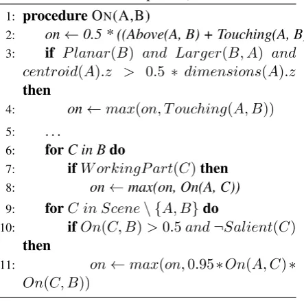
(a)

(b)

Figure 1: An example configuration for the the blocks world domain (a) and the room world do-main (b)

We set up two different annotation tasks – a truth-judgment task and a description task. In the truth-judgment task, the annotator is presented with a screenshot of a scene from either do-main and asked whether the particular relation holds between the given objects (“Is block 1 to the right of block 2?”). The possible qualitative response options form a Likert scale, with five items: “YES”, “RATHER YES”, “UNCERTAIN”, “RATHER NO”, “NO”. In the description task, the annotator is given a screenshot of a scene from ei-ther domain and an object from that scene. The annotator is then asked to describe the object’s lo-cation, in terms of a single prepositional relation to another object in the scene (or two objects, in exceptional cases like between or straddling two objects), so as to identify it uniquely. The annota-tor is encouraged to provide multiple descriptions, if there are several natural ways to pick out the ob-ject uniquely. The list of acceptable prepositions includes the following: above, below, to the right,

to the left, in front of, behind, near, at, in, over, under, between, on, andtouching.3

The objects present in the scenes were selected so as to allow for sufficiently varied configura-tions, combining large immovable items of fur-niture with multiple portable items. There was no specific plan behind the object placement in any scene, except to ensure that the target object can be uniquely described, and the overall con-figuration does not look unnatural or anomalous. To make unique descriptive identification of ob-jects nontrivial, some of the obob-jects, such as chairs or books, were presented in the scenes in several identical copies. Annotators were not allowed to directly refer to the objects by their name (every object in the scene was accompanied by a unique identifier to make it easier for the participant to lo-cate it), but, instead, the participants were asked to use only the type and/or color of the objects when referring to them. Examples of acceptable descriptions include “to the left of another black block”, “between a table and a bookshelf”, “at the bed”, and “on two blue blocks”. In order to au-tomate the process and facilitate gathering of the dataset, an annotation tool was deployed online and about a dozen volunteers (grad and undergrad students from the computer science department) were asked to participate in the preliminary data collection (Fig. 2). Since the task is straightfor-ward they received minimal training; only the re-strictions on the response format (only one prepo-sition, unique identifiability, etc.) were made clear to them.

A number of scenes were created for the pro-posed annotation tasks. For the description task, 151 scenes were created. For the blocks world, each scene was designed to allow three questions (identification of three different blocks), while the more context-rich room world scenes supported 7-8 questions on average. For the truth-judgment task, 192 scenes were designed, with one ques-tion per scene. These 192 scenes are comprised of four variations of 48 basic scenes. The vari-ations are: basic scene (with just the relation ar-gument objects present in the scene), basic scene with bigger frame size (zoomed out), basic scene

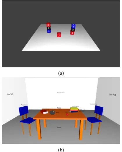
Figure 2: The annotation website. The instructions say ”Where is Blue Chair 1 in the presented scene? Please describe its location relative to other ob-jects.” The instructions are followed by the list of the fourteen admissible prepositions.

with context (additional objects added), and basic scene with context and bigger frame size. The col-lected dataset contains approximately 3500 anno-tations in total, with about 1500 annoanno-tations for the truth-judgment task and 2000 for the description task. It was split into a parameter tuning part and a disjoint test set with the latter containing about 800 annotations, split approximately equally be-tween the description and truth-judgment tasks.

5 Evaluation

The model was evaluated as follows. For the truth-judgment task, the model was used to evaluate the given relation and its arguments. Both the numeri-cal answer provided by the model and the annota-tor’s answer were then transformed to the ordinal scale to compute the agreement coefficient. The human responses were converted from the Likert scale “YES”, “RATHER YES”, “UNCERTAIN”, “RATHER NO”, “NO” into integers 5 to 1, respec-tively. The metric value generated by the model was transformed as follows: Values in[0,0.2)

cor-respond to 1, those in[0.2,0.4)to 2, ..., those in [0.8,1]to 5. For the description task, given a

hu-man description of a target object in relation to a reference object, the model was given the refer-ence object and relation, and was required to iden-tify the object being described.

We used both standard and weighted versions of Cohen’s Kappa as an inter-annotator agreement metric with the weighting penaltyw(i, j) =ki−

jk, where i andj are the ordinal conversions of the responses of human annotators and our system.

The agreement values were computed as follows. First, all pairwise agreement values between an-notators and between each annotator and the sys-tem were computed. Next, the corresponding av-erages (of human-human and human-system pairs, respectively) were found.

For the initial data set (the part used to some extent to tune the model parameters), the accu-racy breakdown was as follows. For weighed Kappa, the average pairwise human-human inter-annotator agreement value was 0.717, whereas the average pairwise system-human agreement metric was 0.682. For standard Kappa, the respective val-ues were 0.536 and 0.479.

For an independent data set used for final evalu-ation, the values were: human-human agreement, weighted Kappa - 0.76, human-system agreement, weighted Kappa - 0.71, human-human agreement, standard Kappa - 0.52, human-system agreement, standard Kappa - 0.49. Again, all these num-bers are pairwise averages. As expected, inter-annotator agreement was not very high.4 _The

somewhat lower system-human agreement is still close enough to human-human agreement to indi-cate the plausibility of our models. Since humans manage to identify referents perfectly well using spatial relations, despite the vagueness of these re-lations, the key question then was how well our models would do for such usages.

relation total occurrences accuracy

to the right of 210 89%

to the left of 212 94%

in front of 118 92%

behind 104 96%

above 81 99%

below 43 98%

over 29 96%

under 135 95%

between 168 93%

at 17 94%

touching 71 93%

near 196 82%

in 31 100%

on 166 90%

Table 1: Fourteen relations, together with the to-tal occurrences within the dataset used for tuning (different annotation) and accuracy per relation.

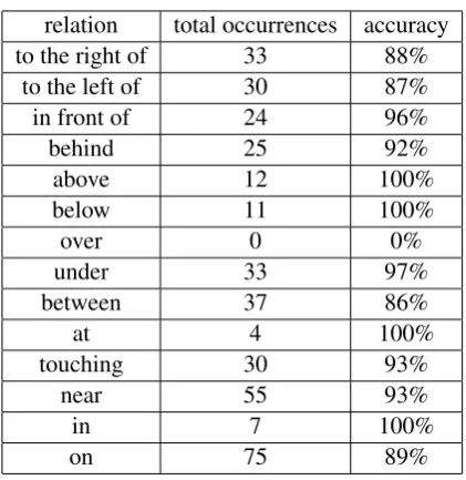
For the description task we computed the accu-racy in terms of the percentage of tests with cor-rectly identified objects. The overall system ac-curacy on the testing data was about 93%; while imperfect, this is an encouraging result. The de-tailed breakdown for separate relations is provided in Table 1.

relation total occurrences accuracy

to the right of 33 88%

to the left of 30 87%

in front of 24 96%

behind 25 92%

above 12 100%

below 11 100%

over 0 0%

under 33 97%

between 37 86%

at 4 100%

touching 30 93%

near 55 93%

in 7 100%

on 75 89%

Table 2: Fourteen relations, together with the total occurrences within the dataset used for final test-ing (different annotation) and accuracy per rela-tion.

6 Discussion and Conclusion

We considered the problem of designing intuitive computational models of spatial prepositions that combine geometrical information as well as some pieces of commonsense knowledge and conttual information about the arguments. In our ex-periments in a blocks world and a room world, we achieved reasonable agreement with human “truth” judgments and quite good agreement in a referential description task. We are not aware of other models that achieved this level of success in comparably diverse environments.

All of the existing methods we mentioned have significant limitations; typically they deal ade-quately with some aspects but fall short on oth-ers. The lexical semantics models in linguistics provide the most comprehensive theory of spa-tial relations as they are used in language. As such they are particularly relevant to natural lan-guage processing applications. However, their biggest drawbacks (at least when they attempt to

address the polysemy of the prepositions) is that they are hardly formalizable and make reference to large amounts of background knowledge about how people interact with the world. Neither hand-crafting that background knowledge nor learning it automatically from data seems feasible at present. On the other hand, research aimed at precise qual-itative spatial models typically puts the emphasis on providing formal frameworks that enable rig-orous inference, rather than on approximating hu-man spatial representations and judgments. Un-surprisingly, this bias results in models that are suitable for certain applications, such as naviga-tion and autonomous problem solving, but not for human-machine interaction. A separate problem is that of reconciling qualitative and quantitative spatial models.

Computational approaches popular today mostly rely on learning the meaning of preposi-tions from data. While they are closer to capturing their natural usage patterns, such models are trained on limited datasets in toy tasks. The generalization capabilities of such models are questionable. In our opinion the path towards comprehensive models of spatial prepositions lies at the intersection of these two major paradigms. The core meanings can be captured by meticulous analysis of the behaviour of the prepositions, while machine learning methods can be applied to adjust the weights of various a priori significant factors and ultimately to learn diverse additional pragmatic factors that influence human judgments in context, but are very hard to describe explicitly. A couple of further insights we gained are worth noting. First, as indicated by the disparity we ob-served between judgments of truth and identifica-tion of referents, experimental design is of utmost importance in this area. Special attention needs to be paid to ensure that the experimental task is nat-ural and sufficiently varied; at the same time, the task should enable isolating the specific meaning aspects of particular prepositions, so that they can be modeled individually. These desiderata are not easily achieved.

onthat we presented above. We did not address the physical aspects of the meaning of spatial preposi-tions in our work. This deficiency will have to be rectified if our models of spatial prepositions are to correspond more fully to our everyday intuition.

Acknowledgments

This work was supported by DARPA grant W911NF-15-1-0542. We thank our annotation team for their contributions, and the anonymous referees for their very useful comments.

References

Eric Bigelow, Daniel Scarafoni, Lenhart Schubert, and Alex Wilson. 2015. On the need for imagistic mod-eling in story understanding. Biologically Inspired Cognitive Architectures, 11:22–28.

Yonatan Bisk, Kevin J Shih, Yejin Choi, and Daniel Marcu. 2017. Learning interpretable spatial oper-ations in a rich 3d blocks world. arXiv preprint arXiv:1712.03463.

Blender Online Community. 2018. Blender - a 3D modelling and rendering package. Blender Foun-dation, Blender Institute, Amsterdam.

BlendSwap.com. 2018. Blendswap.com.

Adrian Boteanu, Thomas Howard, Jacob Arkin, and Hadas Kress-Gazit. 2016. A model for verifiable grounding and execution of complex natural lan-guage instructions. In Intelligent Robots and Sys-tems (IROS), 2016 IEEE/RSJ International Confer-ence on, pages 2649–2654. IEEE.

Alexander Broad, Jacob Arkin, Nathan Ratliff, Thomas Howard, Brenna Argall, and Distributed Correspon-dence Graph. 2016. Towards real-time natural lan-guage corrections for assistive robots. InRSS Work-shop on Model Learning for Human-Robot Commu-nication.

Angel Chang, Manolis Savva, and Christopher D Man-ning. 2014. Learning spatial knowledge for text to 3d scene generation. In Proceedings of the 2014 Conference on Empirical Methods in Natural Lan-guage Processing (EMNLP), pages 2028–2038. Juan Chen, Anthony G Cohn, Dayou Liu, Shengsheng

Wang, Jihong Ouyang, and Qiangyuan Yu. 2015. A survey of qualitative spatial representations. The Knowledge Engineering Review, 30(01):106–136. Istvan Chung, Oron Propp, Matthew R Walter, and

Thomas M Howard. 2015. On the performance of hierarchical distributed correspondence graphs for efficient symbol grounding of robot instruc-tions. In Intelligent Robots and Systems (IROS), 2015 IEEE/RSJ International Conference on, pages 5247–5252. IEEE.

Anthony G Cohn. 1997. Qualitative spatial representa-tion and reasoning techniques. InKI-97: Advances in Artificial Intelligence, pages 1–30. Springer.

Anthony G Cohn and Jochen Renz. 2008. Qualitative spatial representation and reasoning. Handbook of knowledge representation, 3:551–596.

Guillem Collell, Luc Van Gool, and Marie-Francine Moens. 2017. Acquiring common sense spatial knowledge through implicit spatial templates. arXiv preprint arXiv:1711.06821.

Gloria S Cooper. 1968. A semantic analysis of english locative prepositions. Technical report, DTIC Doc-ument.

Bob Coyne and Richard Sproat. 2001. Wordseye: an automatic text-to-scene conversion system. In Pro-ceedings of the 28th annual conference on Computer graphics and interactive techniques, pages 487–496. ACM.

Annette Herskovits. 1985. Semantics and pragmat-ics of locative expressions. Cognitive Science, 9(3):341–378.

Thomas M Howard, Stefanie Tellex, and Nicholas Roy. 2014. A natural language planner interface for mobile manipulators. In Robotics and Automation (ICRA), 2014 IEEE International Conference on, pages 6652–6659. IEEE.

Alice Kyburg. 2000. When vague sentences inform: a model of assertability. Synthese, 124:175–191.

Daniel Lassiter and Noah D. Goodman. 2017. Adjecti-val vagueness in a Bayesian model of interpretation.

Synthese, 194:3801–3836.

Sanjiang Li and Mingsheng Ying. 2004. Generalized region connection calculus. Artificial Intelligence, 160(1):1–34.

Gordon D Logan and Daniel D Sadler. 1996. A com-putational analysis of the apprehension of spatial re-lations.Language and space.

Mateusz Malinowski and Mario Fritz. 2014. A pooling approach to modelling spatial relations for image retrieval and annotation. arXiv preprint arXiv:1411.5190.

R Paul, J Arkin, N Roy, and TM Howard. 2016. Ef-ficient grounding of abstract spatial concepts for natural language interaction with robot manipula-tors. Proceedings of Robotics: Science and Systems (RSS), Ann Arbor, Michigan, USA.

Andrea Tyler and Vyvyan Evans. 2003. The seman-tics of English prepositions: Spatial scenes, embod-ied meaning, and cognition. Cambridge University Press.