warwick.ac.uk/lib-publications
Original citation:
Dyer, Oliver T. and Ball, Robin. (2017) Wavelet Monte Carlo dynamics : a new algorithm for
simulating the hydrodynamics of interacting Brownian particles. Journal of Chemical Physics,
146 (12). 124111.
Permanent WRAP URL:
http://wrap.warwick.ac.uk/86737
Copyright and reuse:
The Warwick Research Archive Portal (WRAP) makes this work of researchers of the
University of Warwick available open access under the following conditions.
This article is made available under the Creative Commons Attribution 4.0 International
license (CC BY 4.0) and may be reused according to the conditions of the license. For more
details see:
http://creativecommons.org/licenses/by/4.0/
A note on versions:
The version presented in WRAP is the published version, or, version of record, and may be
cited as it appears here.
Wavelet Monte Carlo dynamics: A new algorithm for simulating
the hydrodynamics of interacting Brownian particles
Oliver T. Dyer and Robin C. Ball
Department of Physics, University of Warwick, Coventry CV4 7AL, United Kingdom
(Received 22 November 2016; accepted 7 March 2017; published online 24 March 2017)
We develop a new algorithm for the Brownian dynamics of soft matter systems that evolves time by spatially correlated Monte Carlo moves. The algorithm uses vector wavelets as its basic moves and produces hydrodynamics in the low Reynolds number regime propagated according to the Oseen tensor. When small moves are removed, the correlations closely approximate the Rotne-Prager tensor, itself widely used to correct for deficiencies in Oseen. We also include plane wave moves to provide the longest range correlations, which we detail for both infinite and periodic systems. The computa-tional cost of the algorithm scales competitively with the number of particles simulated,N, scaling asNlnN in homogeneous systems and asNin dilute systems. In comparisons to established lattice Boltzmann and Brownian dynamics algorithms, the wavelet method was found to be only a factor of order 1 times more expensive than the cheaper lattice Boltzmann algorithm in marginally semi-dilute simulations, while it is significantly faster than both algorithms at largeNin dilute simulations. We also validate the algorithm by checking that it reproduces the correct dynamics and equilibrium properties of simple single polymer systems, as well as verifying the effect of periodicity on the mobil-ity tensor. ©2017 Author(s). All article content, except where otherwise noted, is licensed under a Creative Commons Attribution (CC BY) license (http://creativecommons.org/licenses/by/4.0/).
[http://dx.doi.org/10.1063/1.4978808]
I. INTRODUCTION
Brownian dynamics (BD) algorithms aim to simplify soft matter simulations by replacing the large number of degrees of freedom in the solvent with known hydrodynamic interac-tions (HIs), which simply need to be calculated between theN
particles of interest at each time step.1
This compares to explicit solvent algorithms that fol-low solvent molecules with some level of coarse graining, despite not being interested in them directly, to let them mediate viscosity and HIs through local interactions. Such methods include molecular dynamics (MD),2dissipative par-ticle dynamics (DPD),3lattice Boltzmann (LB),4–6and multi-particle collision dynamics (MPCD)7algorithms. The
compu-tational cost of these methods, or time taken to run a simulation evolving a system by some physical amount of time, scales lin-early with the total number of particles. This includes particles in the solvent as well as those of interest. For systems of fixed concentration, this leads to the cost scaling asN,8though the overhead cost of moving the solvent molecules limits the feasi-ble system size, especially as the systems become more dilute. When considering a non-periodic system, the scaling rises. An important example of single polymer chains leads toN3ν, with νthe Flory exponent, in order to fit the whole chain inside the simulation box.6
Despite reducing the number of degrees of freedom sig-nificantly, the cost of conventional BD algorithms, which is dominated by the decomposition of the mobility tensor, limits their ability to simulate largeNsystems. Fixman’s algorithm is well known to cut the scaling of this decomposition down
toN2.25from the naiveN3,9and several methods have since
been put forward to reduce the scaling further.8,10It has even
been reduced to or nearNlnNin some cases, although these approaches are only valid for bounded systems,11or introduce errors to allow more efficient computation via particle mesh Ewald techniques12,13or sparse arrays.14
In this work, we present an entirely different approach to BD, using a Monte Carlo (MC) algorithm to bypass explicit calculations with the mobility tensor altogether. To date, MC methods in the field have been used primarily to study equi-librium properties since they have not accounted for HIs. A variety of different particle movement schemes have been used, including simple methods moving individual particles15 and evolving the system with torsional rotations of bonds in polymers.16–18So-called bridging moves have also been
intro-duced to handle branching polymers,19,20and more recently
“event-chain” algorithms have been introduced to handle hard sphere particles.21,22
An important bridge between the MC methods above and our hydrodynamically coupled method below lies in the work of Maggs.23Maggs introduced spatially extended correlated MC moves which he tuned to maximise the equilibration rate of a simple fluid system. He did not target HIs per se, but he was led to motion of the same scaling with arbitrary moves. We focus on moves described by wavelets, a class of function that has seen use in many areas of physics, particularly for signal processing because they form a(an) (over) complete, localised basis that allows temporal changes in a signal to be identi-fied.24,25The development of wavelet theory is catalogued in
Ref.26. For this work, their role as basis functions enables us to
re-express the mobility tensor in a form readily transferable to a MC simulation and hence we call the method “Wavelet Monte Carlo dynamics” (WMCD). We will show that this approach leads to a cost scaling that is at worstNlnNper physical unit of time with a very competitive prefactor and no assumptions on the system beyond those already in basic BD algorithms.
In SectionIIIwe begin with sketch calculations to high-light how HIs and the cost scaling arise in WMCD without needing the full details. SectionIVaddresses the background physics and mathematics required for the method before Sec-tionVexplains the wavelet method in full. SectionVIdescribes a necessary modification to include occasional plane wave moves, before results of simple validation simulations are given in SectionVII.
II. NOTE ON SYSTEMS, UNITS, AND HARDWARE
For the data given in this paper, but not required by the theory, we have simulated polymeric systems in a good sol-vent. The polymers are represented by bead-spring chains with finitely extensible non-linear elastic (FENE) springs and the Weeks-Chandler-Anderson (WCA) potential acting between all particles at positionsri,
UFENE=− 1 2kFENER
2 0 ln
1−(rij/R0)2
, (1)
UWCA=4*
, σ
rij
!12
− σ rij
!6
+ 1 4+
-, (2)
forrij=|rij|=|ri−rj|<R0, 21/6σ, respectively.
We adopt as length and energy units 21/6σ and and denote non-dimensionalised quantities with a bar. Therefore, to match physical systems in Refs.6and8for benchmarking performance, we use ¯σ=2−1/6, ¯=1, ¯kFENE=7×22/6, and
¯
R0 = 2×2−1/6. Matching hydrodynamic radii of individual particles,a, leads to the minimum wavelet radius (introduced in Section V D) ¯λmin = 0.700, while the thermal energy is
kBT =1.2.
We define our unit of time to be the time over which com-pletely isolated or non-interacting particles are expected to have diffused by their own radius,
τ=πηa3/kBT. (3)
By requiring the same viscosityη as used in Refs.6and8, which will only appear implicitly in our algorithm, this unit of time is 4.04 times smaller than in those papers.
Finally, to match the systems in Ref.8, whenever a system is called “semi-dilute” it consists of polymer chains of length
Nb= 10 beads and a global bead concentrationN/L¯3=0.625, whereLis the side length of our simulation box.
All data were obtained using the GNU Compiler Collec-tion (gcc) compiler with optimisaCollec-tion -O3 on a single CPU on an Intel Core2 Quad CPU Q9400 at 2.66 GHz.
III. METHOD SKETCH AND MOTIVATION
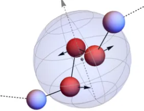
We seek a MC algorithm that produces hydrodynamics in a simple and efficient way. The moves considered are dis-placements inside spheres of radiusλcentred on positionb, chosen from probability density functions (PDFs)PλandPb|λ,
respectively. Here we have anticipated someλ-dependence in the distribution for b. The orientation of these moves, ˆp, is unbiased so that average motion is only induced by non-zero forces weighting the Metropolis test. An example of such a move is depicted in Fig.1.
A move will only contribute to the correlated motion of particlesiandjif it encloses both of them, requiring 2λ>rij and forbto land in a volume of orderλdinddimensions. The contribution from a given move therefore has the piecewise form
D
δriδrj
E
∼
0 for 2λ<rij Pb|λλdA24for 2λ>rij
, (4)
whereA4is a displacement amplitude that is related to strain
by ε ∝ A4/λif, for simplicity in this section, the strain is
assumed to be uniform over the move. In that case, the estimate for the change in energy over a move containingnparticles is
∆Uest∼nε2, which we are constrained by a Metropolis test to avoid being large compared tokBT. This setsA4∼λ/
√ n. ForPb|λ we note that moves with n = 0 contribute no
particle motion and are desirably avoided altogether. Those withn>1 can be chosen by first picking a particle at random and then choosingbat random within distanceλ.Pb|λis then
exactly proportional ton/(Nλd) since each of thenparticles could have led to that centre being chosen.
Finally we pickPλ ∼ λ−d−1, so that integrating Eq.(4)
over radii we have
D
δriδrj
E
∼ ∞
rij/2
dλλ−d+1/N ∝rij2−d/N, (5)
matching the required form for hydrodynamics ind dimen-sions.
We now know the algorithm produces the desired dynam-ics so we turn our attention to estimating the computational cost to evolve our system by a physical amount of time. This will be equal to the cost per move divided by the time evolved per move. The time factor comes from the previous result, using Brownian motion to set it proportional tor2−d
ij δtso that we have a time evolution per move going as
δt∼1/N. (6)
[image:3.594.357.498.598.707.2]Meanwhile, the cost per move of radiusλis of order the expected number of particles involvedn(λ), so the increment
FIG. 1. Schematic diagram of a wavelet move on a section of polymer. The
dashed arrow represents ˆpand the central dot marksb. The particles enclosed
in the wavelet move according to the vectorA4w, introduced in SectionIV A,
in the computational cost is given byδC=c∫ dλPλn(λ), with
cbeing the cost per particle. The homogeneous case has the cost integral diverging logarithmically, leading to
δC
δt ∼cNlnN. (7)
The factor ofN here simply reflects the distribution of com-putational effort across the system, while lnNwill be seen in SectionV Fto stem from an increase in allowedλvalues. It is also shown that for a fractal system, such as a single polymer chain, the logarithm is no longer present.
The method outlined above is therefore very simple, with a favourable cost scaling compared to conventional BD and without the solvent degrees of freedom of explicit solvent methods. The rest of this paper describes the method in detail ford= 3.
IV. MOBILITY TENSORS
We focus on the low Reynolds number limit in which the dynamics of the fluid solvent is governed by the Stokes equations. For simplicity, we assume that we have spherical particles subject to no applied torques, so the dynamics in the system reduces to interrelating the particle velocities,vi, to the applied forcesFj, the latter including interparticle forces. In general, this is given by
vi=
X
j
Gij·Fj+δvi, (8)
whereGis the mobility tensor and the superposability of the velocity response follows from the linearity of the Stokes equations. The contribution from random thermal fluctua-tions, δvi, have covariance set by the fluctuation dissipa-tion theorem (FDT), which in the Stokes limit reduces to
D
δvi(t)⊗δvj(t0)
E
= 2kBTGijδ(t −t0). In practice, we need to implement displacements across a small but non-zero time intervalδt, in terms of which this becomes
D
δri⊗δrj
E
=2kBTGijδt. (9)
In general, the mobility tensor depends on the entire config-uration of particle positions and here we have to simplify, following other workers in using the leading dilute limit expressions. Thus for the self-terms, with i= j, we take the Stokes formGii =I/6πηa, whereais assumed monodisperse for the simplicity of exposition. For the cross terms, we have
Gij(ri,rj)=g(ri−rj) when the interference of third particles is ignored, and then to leading order in powers of separationr
= |rirj| we obtain the Oseen tensor,27
gOseen(r)=O(r)= 1
8πηr(I+ ˆr⊗ˆr) , (10)
corresponding to particles comoving with the bare solvent response, and as a result∇ ·gOseen(r)=0.
As is well known, the Oseen tensor alone does not assure a mobility matrix with non-negative eigenvalues28(crucial for the FDT result), so some modification must always be taken at smallrto remedy this. It has become standard in the recent literature to use the Rotne-Prager (RP) form.29This incorpo-rates the next-leading power of distance, which also turns out
to be divergence free,
gRP(r)=O(r) + 1 12πηr
a
r 2
(I−3ˆr⊗rˆ) , (11)
forr >2a, with a branch for 06r62agiven by
gRP(r)= 1 6πηa I−
3r
32a(3I−rˆ⊗ˆr) !
. (12)
In WMCD we implement the Oseen tensor modified by a cutoff in the wavelet spectrum. This is positive definite and in Section V G we show that it can lead to a tensor very close to gRP. It should be noted that whilst these modifica-tions render the total mobility tensor positive definite, they still under-represent the reduction in mutual mobility of two particles at a close approach, for which ˆr·g·rˆshould match the self term 1/6πηaasr→2a.
A. Wavelet representation of the Oseen tensor
Our method is an adaptation of the continuous wavelet transform in three dimensions, itself based on the identity for the Dirac delta function
δ(ri−rj)=Nδ
dλ
λ
d3b λ3
1
λ34
ri−b
λ !
4 rj−b λ
!
. (13)
The choice of “mother wavelet” shape is surprisingly arbi-trary, with real wavelets constrained only by the formal requirements25
d3x4(x)2 <∞, (14)
d3x4(x)=0. (15)
The normalising front factor is then given by the wavelet Fourier transform ˜4(k):N−1
δ =(2π)2∫ d3kk−3|4˜(k)|2. For this work, it is advantageous to impose additional constraints. The first is to limit the support of4so that
4(x)=0 for |x|>1. (16)
Then it is clear that4( (r−b)/λ) is non-zero only over a region of radius, or “scale”,λcentred onb.
Next we modify Eq. (13)in two ways. First we make the wavelet a vector valued function, w( (r−b)/λ, ˆp), with additional input “polarisation” variable, ˆp. We require these wavelets to be divergence-free,
∇ ·w(x, ˆp)=0, (17)
so thatginherits this property below. It is this constraint of the wavelet being transverse which forces us to supply ˆp. Our vector wavelet can now be thought of as a flow field in the vicinity ofbextending over a length scaleλ.
Our second modification is to change the explicit power ofλin Eq.(13)so that the dimensions match that of the Oseen tensor. This then leads us to consider
g(ri−rj)=Ng
dλ λ
d3b λ3 d
2pˆ
×1
λw ri−b
λ , ˆp !
⊗w rj−b λ , ˆp
!
InAppendix Awe show that this is exactly equal toO(ri−rj) whenλis integrated from 0 to∞and with an appropriate choice of the constantNg.
Equation(18)is more enlightening when expressed as an expectation value. In doing so, we introduce a wavelet ampli-tude A4, which subsumes all constant factors but may also
depend on the wavelet parameters as well. This dependence is found in SectionV C, but for now we assume it is known and write
O(ri−rj)=
* A4w
ri−b
λ , ˆp !
⊗A4w
rj−b
λ , ˆp ! +
λ,b,Dp
,
(19)
where subscripts on the angle brackets indicate quantities aver-aged over. These subscripts are left implicit in later results. Finally, comparison between Eqs.(9) and(19) immediately identifiesA4w( (r−b)/λ, ˆp) as the displacementδr.
V. DESCRIPTION OF THE WAVELET METHOD
With the expectation value interpretation in Eq.(19), we do not need to compute the integral for each particle at every time step and can instead sample wavelets with appropri-ate distributions forλ,b and ˆp. As these moves add up, the correlated motion of particles reproduces that of the Oseen tensor with thermal noise entering via the stochastic move generation.
The details of how this is implemented are given below and inAppendix D, but the basic structure of the algorithm follows the process:
(1) Generate wavelet parameters from their distributions. (2) Provisionally move particles according to the resulting
wavelet.
(3) Calculate the energy change,∆U, caused by this move and accept or reject it with a Metropolis probability
Pacc=min(1,e−∆U/kBT). (20) The process is then repeated for a desired number of moves.
In the Metropolis test, there is no need to include a term for the Jacobian of the move, as per Maggs,23because we will only consider moves with divergenceless flows.
A. Choice of mother wavelet
The restrictions in Eqs.(14)–(17)still leave a choice for
w. In this article, we satisfy these conditions by using the form
w(r, ˆp)=
(
ˆ
p× ∇φ(r) for |r|61
0 for |r|>1 , (21)
for some scalar functionφ.
We also choose to limit ourselves to continuous wavelets so that the strain tensor is finite everywhere. This is required by neither wavelet theory nor the algorithm, but does simplify some of the analysis. Further simplification comes by abbre-viating themth moment of the square of the Fourier transform ofφto
Mm≡ ∞
0
dk kmφ(˜k)2. (22)
For the data in this article, we have used the “tapered wavelet”, which in spherical polar coordinates (r,θ,ϕ), and polarisation vector along the z-axis (θ=0), is given by
w(r, ˆz)=rsinθ(1−r) ˆϕ for r61. (23)
The associatedφand its Fourier transform are
φ(r)= 1 2r
2−1 3r
3−1
6 forr61, (24)
˜
φ(k)=4πk−65ksink−(k2−8) cosk−8. (25)
B. Distributions of wavelet orientation and centres
With the mother wavelet chosen, we now need to deter-mine the distributions from which to pick the parameters. For ˆp
we take an isotropic distribution withP
Dp=1/4πand wavelet
amplitudeA4independent of ˆp.
The PDF forbis more involved as we want to avoid spend-ing CPU time on moves that contain no particles and hence do not evolve the system of interest. To ensure all wavelets con-tain at least one particle, we first pick a particle, all with equal probability, and then chooseb uniformly inside a sphere of radiusλcentred on this particle.
This approach introduces biases that need to be accounted for. First, the probability of choosing a position inside a volume element is inversely proportional to the volume of the sphere. Similarly, the chance that any given particle is chosen is inversely proportional to N. Last, if the resulting wavelet contains n particles, there must have been n pos-sible ways to have chosen it, and hence the probability is increased by this factor. All combined, we have the PDF forb
as
Pb|λ(λ,n(b,λ))=
3 4πλ3
n
N. (26)
C. Choosing the wavelet amplitude
Before the PDF forλcan be determined, we need to know the form ofA4. To find this, we wantPacc, and hence∆U, to
be as constant as possible over all moves so the distribution of
λis correctly reflected in the accepted moves.
An estimate of∆U can be made with the strain energy associated with a move
∆Uest= 1 2µ
3n
4πλ3
d3rε:ε+ε:εT, (27)
where µ is a system dependent particle interaction energy expected to be of orderkBT in soft matter systems and lead-ing us to estimate the local shear modulus as 3µn/(4πλ3).ε is the move’s strain tensor, and “:” denotes a double dot prod-uct. On the assumption of small displacements, we use the infinitesimal strain tensorε=A4
∇w+ (∇w)T/2.
∆Uest =µ
n
λ2
A2
4
(2π)3M6 (28)
for any wavelet of the form in Eq.(21). For this to be constant over moves, we must choose
A4(λ,n(b,λ))=A0λ/ √
n, (29)
withA0a dimensionless tuning parameter that scales the max-imum rotation angle of the wavelet vector field, and thus must be kept small enough to keep the infinitesimal strain approx-imation valid. To maintain simplicity in our results, we use
A0 as a completely free parameter, but we comment that, via Eq.(28), it is fully defined such that
∆Uest
kBT = µ
kBT M6 (2π)3A
2
0, (30)
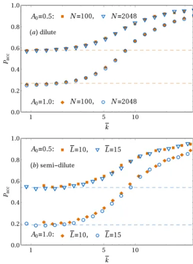
highlighting the contributions from the choice of mother wavelet (M6), the system being simulated (µ/kBT), and the energy scale we are really choosing (∆Uest/kBT). This inter-play is seen in Fig. 2, with both increasing A0 and system density, i.e.µ, increasing∆Uest, and hence decreasingPacc.
Fig.2also reveals that choosingA4as per Eq.(29)leads
to constantPacconly asymptotically, where it limits to a value
Paccasym. For small wavelets, the strain energy estimate is inac-curate as it requires both particles in an interacting pair to be displaced, which is less likely whenλis small, to see a relative displacement from∇wrather thanwitself. This results in an overestimate of∆Uas evidenced by the rise inPacc. Ideally one would like to modify the distribution of λin attempted moves to compensate for the bias observed inPacc, but to do so analytically would be complicated. A simpler and system independent approach is to keep the form ofA4in Eq.(29),
[image:6.594.74.263.578.706.2]which already guarantees thatPaccdoes not drop too low, and use theλ-recycling scheme described at the end ofAppendix D. This scheme is still an imperfect correction for the influ-ence ofPaccon diffusion rates as it fails to take account of any system dependence onband ˆp. It is therefore advantageous to reduce the variation observed inPacc, which can be achieved by loweringA0 as seen in Fig.2. Thus increased dynamical fidelity is available in return for the increased computational cost of making smaller displacements per move, and in this respectA0 can be viewed as the WMCD analog of the time
FIG. 2. Acceptance probabilities over the spectrum of wavelet radii at dif-ferent move amplitudes. The dilute data used an isolated polymer chain with
N= 2048. The dashed lines are only to emphasize the asymptotic behaviour,
while the markers at ¯λ=−1 indicate the averagePaccover all wavelets.
step size of other algorithms. We also anticipate that switch-ing from a Metropolis to a Glauber test,30and further to smart MC,31,32will see reductions in the variation inP
acc.
D. Distribution of wavelet radii
WithA24,P
Dp, andPb|λidentified, we can now determine
Pλfrom Eq.(18)by requiring
λ−5∝PλPb|λPDpA
2
4. (31)
We therefore use the PDF
Pλ(λ)=Nλλ−4, Nλ=3(λ−min3 −λ−max3 )
−1
, (32)
when normalised betweenλminandλmax. The effect of using these finite bounds instead of (0,∞) is discussed in Section
V G. For now we simply comment that a finiteλminis desir-able as it regularises the singularity in the Oseen tensor at
r → 0 and gives us a particle radius viaa = λmin/λa, with
λa a constant dependent only on the choice of the mother wavelet. λmax is required when considering a simulation in a finite box of side lengthL, where we do not want wavelets to overlap with their periodic images due to the additional com-putational effort involved in applying multiple displacements to individual particles.
For a homogeneous system, an alternative method can be used in SectionV B, wherebybis chosen uniformly across the box so thatPb|λ=1/L3, independent ofλ. In this case, it
is sufficient to consider the meanhni, using the global rather than local density. This leads toA4=A0L3/(N
√
λ) and, again, Pλ=Nλλ−4.
The rapid decay of Pλ with either approach means that
small radius moves dominate. This is reflected in Fig.2with the meanPaccbeing significantly higher than the asymptote.
E. Time evolution per move
Next we need to know how much physical time passes dur-ing a simulation, for which we calculate the expected displace-ment squared of any given particle in a single move, Dδr2
i
E
. Using the same approach as inAppendix B, this simplifies to
D
δri2E= 2A
2 0M4 (2π)3NNλ(λ
−1 min−λ
−1
max). (33)
The simulated time increment in a single move,δ¯t =δt/τ, is
then
δ¯t= D
δri2E a2 =
2A2 0M4λ2a (2π)3N
Nλ
λ3
min
1− λmin
λmax !
. (34)
This is consistent with the claim thatA0, which is the only free parameter ifλmaxis taken as large as the simulation allows, is analogous to the choice of the time step.
F. Computational cost
We now come to calculating the computational cost. Here we consider a system with fractal dimensiondf, so that the expected number of particles in a move is proportional to (λ/s)df, withsthe mean separation between near-neighbouring particles.
average cost per particle per move,c, and multiply this by the expected value ofnto find the total cost per move. Dividing this by the time advance per move in Eq.(34), we have cost per unit dimensionless time
dC d¯t ∝
1 δ¯t
D P−acc1Ec
λmax
λmin
dλPλ(λ/s)df. (35)
HereDP−1 acc
E
, defined as
D P−acc1E≡
λmax
λmin
dλPλλdf/Pacc(λ)
,λmax
λmin
dλPλλdf , (36)
handles the additionalλ-dependence coming from ourλ recy-cling scheme. Its value lies between 1 and 1/Paccasym, itself of order unity, and limits to this upper value asλmax → ∞. Its effect on the estimated scaling is therefore small and we will treat it as a constant.
1. Cost of homogeneous systems
When the system is homogeneous or in a poor solvent so thatdf= 3, the integral evaluates to a logarithm ands3=L3N. The cost then goes as
dChomo
d¯t ∝N
2
D P−1
acc
E c
A20M4λ2a
λmin
L !3
ln(λmax/λmin) 1−λmin/λmax
. (37)
For systems with fixed global density andλmax ∼L ∼N1/3, this reduces toChomo∼NlnNper unit of time.
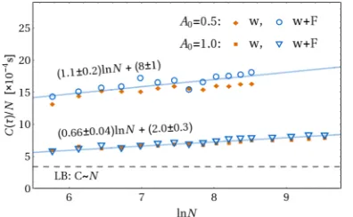
Fig.3 shows cost timings in semi-dilute homogeneous systems which confirm theNlnN scaling. This is true also for the wavelet plus Fourier (w+F) data in this figure, which includes moves described in SectionVIthat only add a minor cost. The following discussion therefore applies to either pure wavelet or w+F data equally.
Because the lnN factor originates in λmax, and hence sees only the asymptotic acceptance probability Pasymacc , the coefficients of the lnN terms in Fig.3vary as 1/(A2
[image:7.594.45.289.103.213.2]0P asym acc ). ReadingPasymacc from Fig.2 predicts a ratio of coefficients of approximately 1.5, agreeing within the error margins in Fig.3. Also in Fig.3, the cost for the LB algorithm for identical semi-dilute systems is seen to be a factor of order 1 times faster
FIG. 3. CPU cost per particle to evolve semi-dilute (homogeneous) systems by a single time unit. The dashed line indicates LB timings from Fig. 8 in
Ref.8, which used identical systems, rescaled to our time unit. Timings for
both pure wavelet (w) and periodic wavelet plus Fourier (w+F) algorithms,
the latter described in SectionVI, are shown for comparison.
than the WMCD algorithm, with the exact factor depending on bothA0andN. (The equivalent BD costs are several orders of magnitude larger.8) Here we note that a fair comparison
would use the same hardware for each algorithm, which was not done here, and the ratio between the costs is therefore only a rough indicator of their relative performance. Moreover our code was far from optimised with particle neighbour lists (the dominant contribution to the cost) being recomputed every move rather than updated only as required; we did not exploit multiple processors, and we compiled with just the standard gcc compiler. Finally, we expect gains relative to LB in semi-dilute systems with longer chains, which are less dense than the systems used in this comparison and consequently the LB algorithm’s explicit solvent would incur an additional cost.
2. Cost of fractal systems
Whendf <3, as in the case for a single polymer chain in good (df= 10.588) orθ(df= 2) solvents,27the cost integrates to
dCfrac
d¯t ∝N D
P−1 acc
E c
A20M4λ2a
λmin
s !df
1−(λmin/λmax)3−df 1−λmin/λmax
. (38)
This time sis taken as the bond length between beads and is set by the potentials between particles. Forθsolvents, the
λmaxdependence cancels, while it is only significant for small systems in the good solvent. In either case we are left with
Cfrac∼N.
This is shown in Fig. 4 where the observed scaling is slightly faster than the theoretical linear scaling inN. We sus-pect that the discrepancy is due to our use of the cell index method,32which introduces small changes in the cost of iden-tifying moving and interacting particles as the chain length increases. For the same reason, the cost is actuallyL depen-dent with the optimalLincreasing withN. For the data in Fig.
4, we usedL= 50 for all data points, and hence the costs given are not optimal.
[image:7.594.70.268.573.695.2]Again, in comparison with other algorithms the differ-ences in hardware should not be forgotten, but in the dilute regime the wavelet algorithm is seen to be much faster than conventional BD for all but the shortest chains, while the LB algorithm is now more expensive because of the many solvent molecules.
FIG. 4. CPU cost to evolve systems with an isolated polymer of lengthNby
a single time unit with the pure wavelet (w) and infinite wavelet plus Fourier (w+F) algorithms. The systems considered were identical to those in Fig. 11
in Ref.6, and the dashed lines indicate the BD and LB timings from that plot,
[image:7.594.333.524.574.696.2]G. Effect ofλmin andλmaxon the mobility tensor
So far the effects of using the finite bounds λmin,λmax
have only been stated without proof. To calculate the effects, we first take the Fourier transform of the wavelet repre-sentation of the Oseen tensor, as per Appendix A, substi-tute in the wavelet form in Eq. (21), and impose the finite limits on the λ integral. This results in the Fourier space tensor
˜
O4(k;λmin,λmax)=
4πA20
3k2
I−kˆ⊗kˆ
kλmax
kλmin
dq q3φ(˜q)2. (39)
The inverse Fourier transform then gives the tensor simulated by the algorithm in a form that more clearly shows its characteristics. With limits (kλ0,∞) this is found in
Appendix Cto be
O4(r;λ0,∞)=
A20
3πr ∞
0
dq q3φ(˜q)2
(I+ ˆr⊗ˆr) Si (Q)
+ (I−3ˆr⊗rˆ)sinQ−QcosQ
Q2
, (40)
whereQ=qr/λ0and Si is the sine-integral function Si (Q)= ∫0Qdt sint/t. The full tensor is then
O4(r;λmin,λmax)=O4(r;λmin,∞)−O4(r;λmax,∞), (41)
which approximates the Oseen tensor between λmin and
λmax, with the regularisation of the singularity and missing correlations for separations larger thanλmax.
To calculate the regularisation at rij → 0, and hence find the particle hydrodynamic radius, we consider the case whereλmax → ∞. This choice anticipates the modification in Section VI. We then associate Eq. (40) with the self-and cross-terms in Section IV, taking the limitsr → 0 and
r → ∞, respectively. In the former limit, the square brackets in Eq.(40)become (4/3)QI, while for the latter they become (π/2)(I+ ˆr⊗rˆ). Since this yields the expected tensor struc-tures, it is sufficient to equate the scalar factors and then solve the 2 equations, giving the ratio
λa ≡
λmin
a =
2 π
M4
M3
. (42)
Hence and as previously claimed,λminis exactly proportional to the particle radius so long as the momentsM3andM4exist. For the tapered wavelet,λa=((9/8)−ln 2)−1≈2.316.
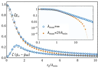
Fig. 5 shows both radial and angular elements of the simulated mobility tensor, measured from correlations in par-ticle displacements, plotted alongside curves derived from Eq.(41). The finiteλmaxdata show long range deviation from
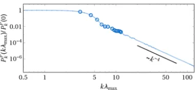
rij−1 behaviour. Intuitively this must happen as any particles separated by a distance larger than 2λmaxcannot possibly have correlated motion due to never being in the same move. Asλmax increases, the long range correlations are more accurately sup-plied, limiting to the correct 1/rbehaviour of theλmax → ∞ data, obtained using the Fourier moves described in Sec.VI.
[image:8.594.330.524.44.179.2]Note that the correlations are very close to those of the RP tensor across both of its branches. As the RP tensor is already an approximation at smallrij, modifying the method to
FIG. 5. Plots of simulated mobility tensor elements normalised byζ=6πηa
with the value ofλmaxgiven in the legend. Theoretical curves from Eq.(41)lie
underneath the data and curves for the full RP tensor are also shown (dashed)
for comparison. Forλmax=29λminthe data forζ(grr−gθ θ) are not shown:
they overlay theλmax=∞data over the whole range. The inset showsζgrr
using logarithmic scales.
explicitly replicate this tensor is not expected to be worthwhile, although we note that it is possible to do so using Fax´en’s laws.33
VI. ADAPTATION TO INCLUDE FOURIER MOVES
We now describe how to modify the algorithm to correct for finite λmax by addingO4(r;λmin,∞) back into Eq. (41).
This is achieved using essentially the same approach but using plane waves as our moves instead of wavelets.
Although it did not matter for wavelets because λmax
ensured that periodic images would not overlap, whether we are considering an infinite or periodic system is now important, and the corresponding tensors will be denoted asO∞F(r;λmax) andOPF(r;λmax). Similarly, other boundary condition depen-dent quantities will be distinguished with these superscripts, and equations that apply for either will leave the superscript off of these quantities.
We start by writing these tensors in the plane wave basis, which is none other than the Fourier transform, so we have
˜
O∞F(k;λmax)=O˜4(k;λmax,∞), (43)
which can be read directly from Eq.(39).
For the periodic case only the commensurate wavevectors are represented, leading to
˜
OPF(k;λmax)= 2π
L !3
III(k) ˜O4(k;λmax,∞), (44)
III(k)≡X
`
δ3
(k−k`), (45)
withk`=(2π/L)(`x,`y,`z) and all`∈ℤ.
The inverse Fourier transforms can be re-expressed in the expectation value form by recognising (1−kˆ⊗kˆ)=2heˆ⊗eˆi
De,
with ˆea unit vector perpendicular to ˆk. To re-expresseik·rij, we note that ˜O4(k;λmax,∞) is even in k, so we can replace
the complex exponential with
cos(k·rij)=2
D
cos(k·ri+Φ) cos(k·rj+Φ)
E
FIG. 6. Schematic diagram of how a Fourier move displaces all particles in the system. The plane wave surface indicates the vector field, which is
perpendicular tokand spans the entire system.
In both cases the distributions are uniform so thatP
De=PΦ =
1/2π, and we finally have
OF(rij)=hAFcos(k·ri+Φ)ˆe⊗AFcos(k·rj+Φ)ˆeiΦ,De,k
(47)
withAF filling the same role as A4 did for wavelet moves.
We therefore have Fourier moves causing displacements δr=AFcos(k·r+Φ)ˆe, as seen diagrammatically in Fig.6, and the infinite and periodic versions differing only in their distributions overk.
The rest of this section follows loosely Sec.V.
A. Choosing plane wave amplitude
Similarly to SectionV C, we desireAFto be chosen such that∆Uis independent ofk. Further to this, we want the change in energy to be equal to that of wavelet moves.
In a Fourier move, the whole simulation box sees a dis-placement, so the move volume is L3 and n = N. Any L -dependence will cancel so this approach is still valid for the infinite case. The strain energy estimate is therefore given by
∆Uest= 1 2µNL
−3A2 Fk
2
box
d3rsin2(k·r+Φ)
=1 4µNA
2 Fk
2, (48)
settingAF(k)=2k−1
p
∆Uest/µNwith∆Uest/µtaking the same value as set byA0in Eq.(30).
Fig.7verifies that choosing this form does indeed lead to a constant acceptance probability, at least for smallkmodes which will end up dominating the distribution. For these low frequency moves, comparison with the wavelet asymptotic val-ues, seen again as dashed lines in Fig.7, confirms that equating Eqs.(28)and(48)correctly equates the actual energy changes in wavelet and Fourier moves.
At largekthe wavelength is less than the particle sepa-ration and the gradient of the vector field is no longer a good measure of the relative displacements of nearby particles. Con-sequently the strain energy is an overestimate, leading toPacc rising to 1. Similarly to how we recycle the radius of failed wavelet moves, and as described at the end ofAppendix D, we recycle the absolute value ofkof Fourier moves to correct for the variation inPacc.
We now address the divergence ofAFat thek= 0 mode. This mode is left out in the Ewald sum in other methods to enforce zero net force.34For our algorithm, thek= 0 mode has no influence on dynamics within the system and by viewing the system in the centre of mass frame we set the displacements associated with this move to zero. However, because in the
FIG. 7. Acceptance probabilities over the spectrum of plane waves at different move amplitudes. (a) Single chain data using the infinite algorithm. (b) Data for semi-dilute systems with the periodic algorithm. Dashed lines, indicating
the asymptotic wavelet values ofPaccfor equivalent systems, are identical to
the dashed lines in Fig.2.
periodic case this mode has a non-zero probability of being chosen, as is shown in Sec. VI B, we deem these moves be accepted even though they induce no change in the system. Their automatic acceptance coming from∆U = 0 accounts for the slight rise inPaccin the lowestkbins in Fig.7(b).
B. Distributions of wavevectors
With the amplitude chosen, we are now able to determine the distribution of wavevectors. For the infinite case, these are isotropically distributed so thatP∞
Dk =
1/4π, while the radial part picks upk2fromd3k, giving
P∞ k (k)=N
∞ kk
2
∞
kλmax
dq q3φ(˜q)2. (49)
The normalisation simplifies to
N∞ k =3λ
3 maxM
−1
6 . (50)
For the periodic case,III(k) turns the PDF into the discrete set of probabilities
PPk(k`)=NPk
∞
k`λmax
dq q3φ(˜q)2, (51)
where the normalisation, obtained by a sum of this integral over allk`, cannot be expressed in a simple way.
For the tapered waveletPP
kis shown graphically in Fig.8, where thek4decay in the number of high frequency modes, resulting from wavelets already accounting for the short-range correlations these would be contributing, ensures thatNP
[image:9.594.71.262.48.115.2]FIG. 8. Probability of picking Fourier modes in a periodic system in Eq.(51),
normalised by the probability of picking thek= 0 mode. Markers indicate the
lowest discrete modes whenλmax=L/2, starting atk=2π/L.
its maximal value of L/2 all but the k= 0 mode experience this decay and low frequency modes therefore dominate the distribution.
C. The probability of making a Fourier move
It now only remains to determine how often to make a Fourier move, for which we compare the magnitudes of the tensors generated by the missing wavelets with λ > λmax
and the Fourier moves replacing them, after conversion to the expectation value form. Surprisingly we find exact equality, i.e.
D
δri⊗δrj
Eλ>λmax
4 =
D
δri⊗δrj
E∞
F, (52)
when we might have expected the normalisations to introduce a relative factor. It turns out the fixing of the strain energies to be equal, which can be viewed as an operator onhδri⊗δrji, set this factor to 1. This leads us to the remarkable result that, on average, a Fourier move evolves time by the exact amount that a missing large wavelet would have done, regard-less of the value ofλmax. We therefore need to make a Fourier move with the same probability as picking a wavelet with
λ>λmax,
PF∞= λ
3 min
λ3max. (53)
To show that this argument is consistent with the pre-viously found distributions, we explicitly calculateDδr2
i
E
for infinite system Fourier moves. After averaging over space and the trivial ˆk, Φ, and ˆe integrals have been performed, this becomes
D
δri2E∞ F =
1 2N
∞ k
∞
0
dk k2A2F ∞
kλmax
dq q3φ(˜q)2
=2∆Uest
Nµ
3λ3max λmax
M4
M6
, (54)
which is identical to Eq.(33)whenλmax → ∞ andλmin →
λmax, as expected.
In periodic systems, the argument is complicated by the estimated energy for wavelets being invalid forλ>L/2 when
they overlap with their own images, and hence the relative factor,Rsay, has not been fixed at 1. Performing the energy calculation directly is intractable for overlapping wavelets, but the value of R can be found indirectly by comparing the introduced normalisation factors. The wavelet factors are unchanged from the infinite case, so it is sufficient to use the
ratio of introduced factors between the infinite and periodic Fourier tensors, which gives
R= L 2π
!3 NP
k N∞kN∞
Dk
=6π12 L
λmax !3
M6NPk. (55)
To calculate the probability of making a Fourier move, we enforce equal time evolution from Fourier and missing wavelet moves after the same number of wavelet moves withλ<λmax, leading to
PPF=1 +Rf(λmax/λmin)3−1g−1. (56)
Finally we calculate the new value of δ¯t, taking both Fourier and wavelet moves into account. Becauseτis defined for an isolated particle, this will useDδri2E∞
F in both the peri-odic and infinite systems. Since this is identical to the missing contribution ofλmax <λ<∞, it is clear that we can just take
λmax→ ∞in Eq.(34)to obtain
δ¯t= 6A
2 0M4λ
2 a
(2π)3N . (57)
D. Computational cost with Fourier moves
Armed with the frequency at which Fourier moves are chosen, we now calculate the computational cost associated with them. Each plane wave evolves allNparticles, each with a costcas in the wavelet case, byδt∼N−1. For Fourier moves alone then, the cost would scale asN2.
Accounting for the presence of wavelet moves, the Fourier contribution to the cost is weighted by PF ∼ λ−max3 ∼ N−1 for a set of constant density systems. The Fourier moves are therefore subdominant to the wavelet cost, and the previous
NlnN scaling remains, as observed in Fig.3. Similarly the fractal scaling ofN is unchanged ifλmaxcontinues to scale at least as fast asN1/3, which is slower than theNνscaling of the polymer size.
Unlike the Ewald sum in BD simulations, which splits the workload so that the cost of the Fourier space calculation is comparable to the position space part,8there is no requirement
for the total cost of WMCD Fourier moves to be comparable to the cost of wavelet moves. Indeed Figs.3and4both show that the Fourier moves can contribute only a small, if not negligible, fraction of the total cost.λmaxcan be tuned to give comparable costs, but since Fourier moves replace wavelets on a 1-to-1 basis regardless of the value ofλmaxand they always carry the cost of moving every particle, this is not optimal. Rather it is optimal to takeλmax =L/2, or as close as the algorithm’s
implementation allows.
VII. ALGORITHM VALIDATION
A. Chain relaxation
The relaxation of isolated chains of lengthNb= 10 beads with initially stretched or compressed bonds is seen in Fig.9, with a mean-square radius of gyration defined as
D
R2gE= 1
2Nb2 Nb
X
i=1 Nb
X
j=1
D
FIG. 9. Relaxation of an isolated polymer withNb= 10 and WCA and FENE
potentials, for differentA0and initial bond lengths, ¯s(0). The dashed line
shows the value for the same system in Ref.8.
Both stretched and compressed chains relax to the same value as obtained for this system in Ref. 8, confirming the algorithm equilibrates correctly, and therefore that ourλand
krecycling schemes have not violated detailed balance. The figure also shows the same physical relaxation time for the different values ofA0, verifying theA0-dependence in Eq.(57).
B. Chain diffusivity
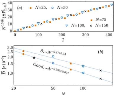
Diffusion of the centre of mass of chains of different lengths is shown in Fig.10(a), where the correct linear relation-ship with time is seen. Note that we are ignoring the difference between short and long time diffusion in the analysis as these basic data are not precise enough to distinguish the few percent between them.35Data at that accuracy are left for future work.
Fig.10(b)shows measured centre of mass diffusion con-stants,D = D∆rCoM2 E/6t, for chains in both good and θ sol-vents, with the former using the same data as in Fig.10(a). For theθsolvent, the WCA potential was turned off and the FENE potential was replaced with the harmonic bond potential (3/2)kFENE(rijr0)2, in which ¯r0=0.9691 was used to match the mean bond length in the good solvent. These sets of data show quantitatively that simulations in both types of solvents lead to expected scaling withNwithin the error bounds on the
FIG. 10. (a) Mean centre of mass displacement squared for isolated chains in a good solvent, scaled to show the theoretical collapse of the data. Every fifth data point has been used from each data set to show this clearly. (b) Measured diffusion constants plotted against the chain length for chains with identical
mean bond lengths in good andθsolvents.A0= 0.5 was used for all WMCD
data, while the star marks the diffusivity measured in a good solvent in Ref.6.
exponent.27The absolute values in the good solvent also agree with previous work, with the value atN = 32 (star) provided by Ref.6lying on the fit of our data. No previous data forθ solvents with these parameters are available for comparison.
The scaling seen in Fig. 10(b) is usually considered asymptotic, requiring long chains to observe. To see why this is not the case with our data, we write the chain diffusivity as per Ref.36,
D= kBT
6πηa
f
N−1+aDR−HI1Eg
= kBT 6πηa
f
N−1+aAN−ν−BN−1+· · ·g, (59)
which has splitDinto terms expressing the sum of hydrody-namic radii of individual monomers and the contribution from the HIs between the monomers.
UsingB= 4.036/s, found for Gaussian chains with a root mean square bond lengths,36as a rough estimate for our sys-tems, and inputting our values ofs≈1 anda ≈0.3, we find
aB≈ 1.2. This leads to a significant cancellation of theN1
terms, whileaA ≈ 1.1 so theN−ν term dominates and scal-ing is expected at smallN. Note that the common practice of neglecting the first term in Eq.(59)would hide this result.
For polymers in the good solvent, there are additional “non-analytic” terms that come from excluded volume inter-actions.36Nonetheless the qualitative result is the same when we use coefficients fitted in Ref.36. While we do not expect the coefficients used here to apply exactly for our systems, it is the near cancellation of theN1 terms that we highlight as explaining the scaling observed, and that we do expect to apply.
C. Finite box effect on self-diffusion
The periodic algorithm should lower the diffusivity because of the extra HIs with periodic images. The simplest check for this is to look at the trace of the mobility tensor in the limitrij → 0, which has been calculated to leading order to vary with the box size as37
Tr[OP(0;λmin)]=Tr[O∞
(0;λmin)]
1−2.837a
L
. (60)
[image:11.594.69.262.525.686.2]By generating correlation curves for Dδr2iE with non-interacting particles, similar to Fig. 5, and comparing the
FIG. 11. Simulated traces of self-diffusion tensors, scaled by the mean trace
of infinite systems for eachλmin, in simulation boxes with ¯Lbetween 5 and
30. The solid and dotted-dashed lines were calculated using Eq.(60).A0= 0.5
[image:11.594.331.525.582.709.2]unscaled values atrij →0, we have confirmed this behaviour as well as the L-independence of the infinite algorithm (see Fig. 11). This figure also confirms that Eq. (57) is indeed appropriate for periodic systems as the measured diffusivi-ties are inversely proportional to how we scale time. Finally, it provides a further verification of Eq.(42)as this determines the value ofaand hence the gradient of the lines via Eq.(60).
VIII. SUMMARY AND OUTLOOK
In this paper, we have detailed the Wavelet Monte Carlo dynamics algorithm, using wavelet and plane wave moves to produce hydrodynamics without explicit decomposition of the mobility tensor. Our algorithm has been shown to closely approximate the Rotne-Prager tensor by starting from the Oseen tensor and removing small radii moves, which in turn provides an explicit particle radius. The distribution of addi-tional Fourier moves, meanwhile, can be chosen to simulate either a periodic or infinite system with the main wavelet part of the algorithm left unchanged.
It has been shown that the computational cost of WMCD scales well to large systems, going asNlnNfor homogeneous systems with fixed particle density and asNfor fractal systems. Both of these have a very competitive prefactor, making it a promising simulation technique for extending the reach of soft matter simulations.
The algorithm has been tested to show that correct hydrodynamic correlations are produced, while the simulated behaviour of isolated polymer chains has been shown to agree with previous work.
For the case of homogeneous systems, our wavelet algo-rithm turns out to be fortuitously well balanced across length scales according to three distinct criteria. First we chose the move amplitudes (Eq.(29)) such that their elastic energy is expected to be of orderkBTleading to move acceptance inde-pendent of the wavelet radiusλ. Second we then found that this leads to computational cost∫ dλ/λuniformly distributed over length scales, leading to the logarithmic dependence in the overall cost (Eq.(37)). Third the time scale for the algo-rithm to build the move correlations across a distancer, which come predominantly from wavelet radiiλ∼r, turns out to be independent ofλ. This last result can be seen from the way the squared move amplitudes haveλ-dependence matching ther -dependence of the cross mobility (Eq.(10)), and it means that the time scale to build up long ranged correlations is of the same order as the time scale for particles to expect to experi-ence a local (small wavelet) move. It is easily checked that the
d-dimensional sketch of the method given in SectionIIIleads to all the same coincidences. The case where the coincidences do unravel is when the distribution of particles is fractal, as with a dilute polymer and locally in a semi-dilute polymer: then the longer wavelet moves are allowed greater amplitude leading to computational cost dominated by small wavelets. There is correspondingly longer build-up time for long ranged correlations, but this is still fast compared to the corresponding polymer relaxation modes.
With the core set out, we plan to develop the algorithm further to include solvent flows. We envision the procedure with this modification to be essentially the same as presented
in this article interspersed with flow-generating moves. So long as the flow moves, however they are implemented, have small enough amplitudes to keep close, interacting particles near equilibrium, even with large scale separations along the chain moved out of equilibrium, we expect the energy estimates in this article to remain valid. Consequently we do not anticipate any change to how we handle the existing moves.
On the computational side, there is scope to improve the current algorithm in several areas. Foremost we can improve the accuracy and reduce the variation in the move rejection rate by switching from the Metropolis to Glauber move acceptance, and also to smart MC in which moves are biased according to the force conjugate to them. There is also scope for the optimisation of choices which already exist, notably the choice of the mother wavelet is yet to be explored. The precise way in which periodic boundary conditions are enforced on the hydrodynamic propagator is another deeper choice where we have followed that of prior work, but it is a choice, for example, we could have chosen to keep only the wavelet moves.
A range of coding improvements also stand to be made. The computational cost could be reduced by tracking particle neighbour lists rather than re-computing them at each move, and computational speed could be increased by a combina-tion of parallel execucombina-tion of multiple non-overlapping wavelet moves and parallelised execution of single large wavelet moves.
ACKNOWLEDGMENTS
This work has been supported by the Engineering and Physical Sciences Research Council (EPSRC), Grant No. EP/L505110/1 (O.T.D.), and the Monash-Warwick Alliance (R.C.B.). The authors acknowledge stimulating discussions with J. R. Prakash and are also grateful to the remaining organ-isers of “Hydrodynamic Fluctuations in Soft-Matter Simu-lations” CECAM/Monash workshop, Prato (February 2016) wherein many helpful discussions were had.
APPENDIX A: SHOWING THE WAVELET
REPRESENTATION GIVES THE OSEEN TENSOR
Here we evaluate the integral in Eq.(18)to show that this reduces to a form exactly proportional to the Oseen tensor. We begin by taking the Fourier transform with respect torirj, leading to
˜
g(k)=
d3re−ik·(ri−rj)g(ri−rj)
=Ng
d2pˆdλ
λ λ
2w˜ (λk, ˆp)⊗w˜(−λk, ˆp) , (A1)
where ˜w(k, ˆp)=∫ d3xe−ik·xw(x, ˆp) is the Fourier transform of the mother wavelet at fixed ˆp.
We next integrate over the wavelet polarisation to obtain
˜
g(k)=4πNg
dλ λW(λk), (A2)
W(k)= 4π1
d2pˆw˜ (k, ˆp)⊗w˜ (−k, ˆp)
which has the explicit tensor structure shown because the con-straint∇ ·w=0 leads tok·W=0. The amplitude factor is set by
2f(k)=Tr [W(k)]= 1 4π
d2pˆw˜ (k, ˆp)·w˜ (−k, ˆp) . (A4)
Reassembling all this and making the substitutionq=λkleads to
˜
g(k)=4πNgk−2(I−kˆ⊗kˆ) kλmax
kλmin
dq qf(q). (A5)
For λmin → 0 and λmax → ∞, this exactly matches the Fourier transform of the Oseen tensor, (1/ηk2)(I−kˆ ⊗kˆ), upon choosing the normalisationN−g1=4πη∫0∞dq qf(q).
APPENDIX B: SIMPLIFYING THE WAVELET STRAIN ENERGY INTEGRAL
The strain energy in Eq.(27)can be simplified by chang-ing the integration variable to x = r/λ, whereupon all the
λ-dependence in the integral factors out viad3r=λ3d3xand ∇ = λ−1∇x, with ∇x the gradient with respect to x. This leaves the integral as a parameter independent number so that
∆Uest∝n/λ2for all mother wavelets. The integral itself reduces to
A24
d3x∇xw:∇xw+∇xw: (∇xw)T, (B1)
in which the left term is readily seen to integrate to 0 by integrating by parts and then using the divergencelessness of our wavelets (Eq. (17)) and that they take the value 0 at their boundary (SectionV A). The integral over the remaining term can be written in terms of the wavelet’s Fourier transform as
A24
(2π)3
d3kk2w˜(k)·w˜(−k). (B2)
We then substitute in the Fourier transform of the wavelet type in Eq.(21), ˜w(k)=i( ˆp×k) ˜φ(|k|), and use ( ˆp×k)·( ˆp×k) =k2sin2θto reach the final form of
8πA24
3(2π)3
∞
0
dk k6φ(˜k)2. (B3)
APPENDIX C: DERIVATION OFO4(r;λ0,∞)
The inverse Fourier transform of Eq. (39), with the q
integral fromkλ0to∞, is
O4(r;λ0,∞)=
A20
6π2
allk
d3keik·rk−2I−kˆ ⊗kˆ
× ∞
kλ0
dq q3φ(˜q)2. (C1)
First, we commute theq andkintegrals, which require a change in their limits. To be able to perform the integral, we also note that ˆk⊗kˆeik·r=−∇ ⊗ ∇k−2eik·r. What remains
is an inverse Fourier transform of a radial function, so the angular integrals over the exponential give the usual result of 4πsin(kr)/kr, so that we have
O4(r;λ0,∞)=
2A20
3π
∞
0
dq q3φ(˜q)2
× q/λ0
0
dk I+∇ ⊗ ∇k−2sinkr kr . (C2)
We now focus on performing thekintegral.
TheIterm integrates directly to Si(qr/λ0)I/r. The other term appears to diverge at thek→0 limit, but it can be split up into an integral with limits (0,∞) minus a finite one over (q/λ0,∞). Although the first of these still appears to diverge, it is exactly what would have been integrated if we had the full Oseen tensor. It is therefore known to be (π/4r)(ˆr⊗ˆr−I).27
Hence we are only left with−∇ ⊗ ∇acting on
1
r ∞
q/λ0
dk k−3sin(kr)= λ
0
2q
f
cosQ+Q−1sinQ
+Q
Si (Q)−π 2
, (C3)
withQ = qr/λ0. Performing the two derivatives obtains the form
Si (Q)−π 2
1
2r(ˆr⊗rˆ−I) +
sinQ−QcosQ Q2
1
2r(I−3ˆr⊗ˆr) .
(C4)
Theπ/2 term cancels exactly with the full Oseen term above, while the remaining terms plus the contribution from the first
Iterm give the final result
O4(r;λ0,∞)=
A2 0 3πr
∞
0
dq q3φ(˜q)2
(I+ ˆr⊗rˆ) Si (Q)
+ (I−3ˆr⊗ˆr)sinQ−QcosQ
Q2
. (C5)
Note that this calculation could have started from Eq.(A5)
for a more general wavelet. In this case, all that need changing areq2φ(˜q)2/3→f(q) andNg →A20.
APPENDIX D: DETAILS OF GENERATING MOVE PARAMETERS
In this section, we detail how the calculations of parameter distributions in this article translate to generating the Monte Carlo moves in a WMCD simulation. We denote numbers gen-erated by a pseudo random number generator byrand, which is always uniform over the range indicated. Where multiple numbers are needed for a single quantity, subscripts are used to distinguish them.
Before any parameters are generated, the move must first choose either a wavelet or a plane wave. For this we generate