Stellar pulsation: a study of the influence of opacity on numerical models

STELLAR PULSATION:

A STUDY OF THE INFLUENCE OF OPACITY ON

NUMERICAL MODELS

Zaki A. Al-Mostafa

A Thesis Submitted for the Degree of MPhil

at the

University of St Andrews

1995

Full metadata for this item is available in

St Andrews Research Repository

at:

http://research-repository.st-andrews.ac.uk/

Please use this identifier to cite or link to this item:

http://hdl.handle.net/10023/14386

STELLAR PULSATION

A STUDY OF THE INFLUENCE OF OPACITY ON

NUMERICAL MODELS

BY

ZAKI A. AL-MOSTAFA

A Thesis submitted for the Degree of Master of Philosophy

at the University of St. Andrews.

June, 1994.

ProQuest Number: 10171293

All rights reserved

INFORMATION TO ALL USERS

The quality of this reproduction is dependent upon the quality of the copy submitted.

In the unlikely event that the author did not send a com plete manuscript and there are missing pages, these will be noted. Also, if material had to be removed,

a note will indicate the deletion.

uest

ProQuest 10171293

Published by ProQuest LLO (2017). Copyright of the Dissertation is held by the Author.

All rights reserved.

This work is protected against unauthorized copying under Title 17, United States C ode Microform Edition © ProQuest LLO.

ProQuest LLO.

789 East Eisenhower Parkway P.Q. Box 1346

AU

Ab s t r a c t

A theoretical study of Population II variables has been carried out using the non­ linear approach and using the more recent molecular opacities of Carson and Sharp (1991) with the atomic opacities of Iglesias and Rogers (1991). The calculations have been done using a computer code created by Dr. T. R. Carson.

More than fifty models have been constructed for different compositions for Hydrogen (X), 0.745, 0.749 and 0.750 and for Helium (Y) fixed at 0.250. These models belong to three types of stars, RR Lyrae, BL Herculis and W Virginis.

The aim of this study was to test the new opacities and compare them with the old ones (especially those of Carson).

Generally the periods of the old and new models are in very good agreement. However, the amplitudes of the new models tend to be fairly consistently smaller than those of the old models, tending towards greater agreement with observation. The new blue edges are shifted redward (toward lower temperature) with respect to the old, particularly for the larger values of the metal content Z, and less for smaller Z.

However, for the same composition all results are in excellent agreement with those of Carson, Stothers and Vemury (1981) using the opacities of Carson

DO...

W jij Parentôy

Wj,

W if.,

^ b a u ^ L t e f ô ^ J a t m a ^ a r a k y

yyiff i^rotker^â a n d ^ iôterây

a i i yi/joôlemô around tke w orid.

Praise be to Allah

The Cherisher and Sustainer of the Worlds,

Then,

I would like to express my deep gratitude to my supervisor Dr. T. R. Carson, who has offered me great deals of his expensive time. Elaborate discussion

with him and his continuous guidance throughout different phases o f this project facilitate my achievement and bring this work to life.

CERTIFICATE

I hereby certify that the candidate has fulfilled the conditions and

regulations appropriate to the Degree of Master of Philosophy

{M.Phil.)

of the University of St. Andrews and that he is qualified

to submit this thesis in application for that degree.

DECLARATION

I, ZAKI A. AL-M

OSTAFA, hereby certify that this thesis, which is

approximately 20,000 words in length, has been written by me, and

that it has not been submitted in any previous application for a higher

degree.

I was admitted as a research student under Ordinance No. 12 on the

October 1992 and as a candidate for the degree of M.Phil. on the

October 1993; the higher study for which this is a record was carried

out in the University of St. Andrews between 1992 and 1994.

Zaki A. AL-Mostafa

In submitting this thesis to the University of St. Andrews I understand

that I am giving permission for it to be made available for use in

accordance regulations of the University Library for the time being in

force, subject to any copyright vested in the work not being affected

thereby. I also understand that the title and abstract will be published

and that a copy of the work may be made and supplied to any bona

fide library or research worker.

>

Co n te n t s

PAGE

INTRODUCTION... 1

CHAPTER 1: PARTA lA-1: P o p u la tio n II C epheids... 3

FARTB lB-1: RR L y ra e S t a r s ... 11

lB-2: BL H e rc u lis S t a r s ... 15

lB-3: W V irg in is S t a r s ... ... 17

CHAPTER 2: 2-1 T h e N o n -L in e a r T h e o ry ... 24

2-1-1: The Pulsation Theory... 24

2-2 THE E q u a tio n s O f S t e l l a r P u ls a tio n ... 26

2-2-1: Th e Basic Equ ations...26

2-2-2: Th e Boundary Conditions... 31

CHAPTER 3: 3-1: T h e M e th o d O f S o lu tio n ...34

3-2: T h e E q u a tio n O f S t a t e ... 45

'U.' ' -? Y \ A'

PAGE I

APPENDIX A: |

A-1: Lig h t, velocity & Ra d ius Curves Fo r Th e RR Lyra e Mo d els...67 1

A-2\ Lig h t, velocity & Radius Curves Fo r Th e BL Herculis m o d e l s... 68

A-3\ Light, v elo city & Radius Curves Fo rthe W Virginis Mo d el s...69 |

APPENDIX B: f

The Ligh t, velocity & r a d iu s Curves Of Th e Decayin g Mo d el s... 70 |

APPENDIX C:

The IR Opa city Ta bles. .71 4

APPENDIX D:

D - h T he L in e a r T h e o ry ...76

D-2: The Eq u a tio n s...76

REFERENCES... 86

In t r o d u c t io n

During the past fifty years the pulsating variables have played an important and rather controversial role in the drama of our unfolding knowledge of the outline and dimensions of the universe of galaxies. So, the object of this study was to model Population II stars using the non-linear pulsation analysis in the hope of obtaining velocity and light curves of similar amplitudes and features to those produced by the real stars. In this study we have used the more recent molecular opacities of Carson and Sharp (1991) with the atomic opacities of Iglesias and Rogers (hereafter, IR) (1991).

This thesis is divided into four chapters and four appendices.

In Chapter One part A, a review of the Population II Cepheids. In part B we review the three types of Population II that have been used in this thesis, these are RR Lyrae, BL Herculis and W Virginis. Therein given the main properties of each type and its importance.

In Chapter Two and Three the non-linear theory and the method of solution of the equations that have been used are described.

In Chapter Four the main results are presented and discussed.

In Appendix A we present the theoretical models for RR Lyrae, BL Herculis and W Virginis. In Appendix B the decaying models are presented.

In Appendix C the IR opacities are presented and compared with the Carson.

CHAPTER

ONE

Chapter ONE

Page-3-lA-l.

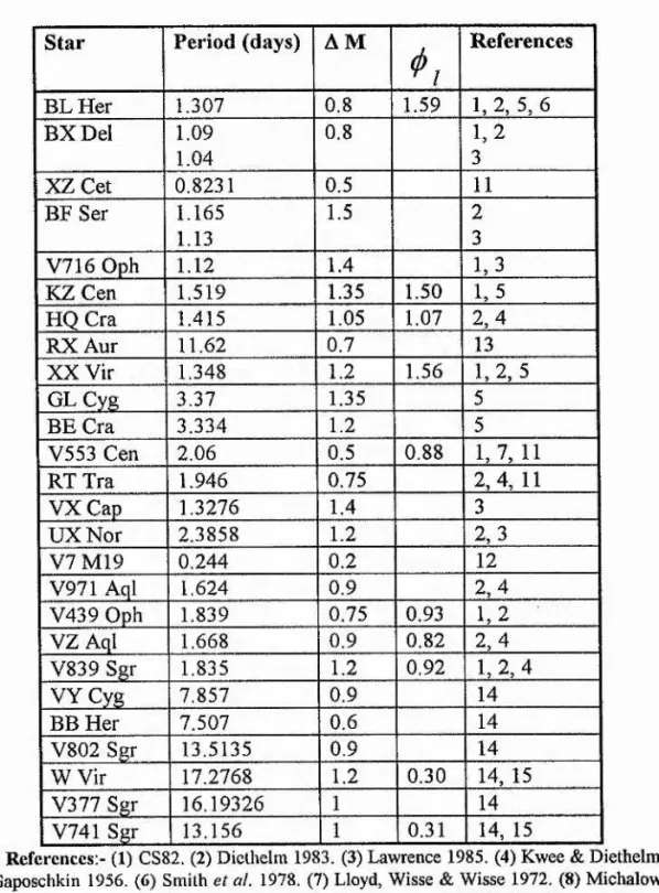
s:-Population II ( Pop II, hereafter) cepheids generally originate from low-mass stars of low metallicity which are undergoing post core Helium (He) burning stage of their evolution (Becker 1985). Pop II are divided into three main categories which are the BL Herculis (BL Her) stars, the W Virginis (W Vir) stars and the anomalous Cepheids, see Table 1-1. Low-mass Pop II stars evolve off the suprahorizontal branch to Asymptotic Giant Branch (AGB) where the Hydrogen (H)-burning shell re-establishes itself and the double burning shell phase begins. When the Hydrogen envelope is nearly exhausted ( <5xlO “^M _{^ sun} ) due to the last He shell flash on the AGB, one or two

Chapter ONE

Page-4-Variable stars in the H-R diagram are classified, based on their observed properties, into distinct types. The underlying mechanism for the variability is generally felt to be due to four different causes (Becker 1986):

1) geometric effects. 2) rotation.

3) eruptive processes. 4) pulsation.

In our thesis the focus will be on the fourth cause.

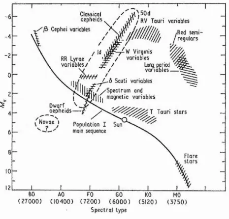
Type II cepheids have periods ranging upward of 1 day (Carson et al. 1981), The discovery of many Type II cepheids led to the introduction of distinct subclasses, such as BL Her, W Vir and RV Tau stars as well as less well defined subgroups such as the anomalous cepheids, which are more luminous at a given period than cepheids found in globular clusters. They (type II cepheids) lie on the H-R diagram between the RR Lyrae variables, at low luminosity, and the RV Tauri and long period variables at high luminosity (Becker 1985). Figure 1-1 shows that RR Lyrae and W Vir occupy roughly the same location in H-R diagram as do the classical cepheids. The long, nearly vertical, region shown on the H-R diagram lying above the main sequence, contains both the RR Lyrae and W Vir , as well as the classical cepheid and other types of pulsating stars. Because of their peculiarities, no strict definition can be given for type II cepheids. It is mostly on the theoretical basis of stellar evolution theory that all the subclasses above are regarded as Pop II (Kovacs & Buchler 1988).

Chapter ONE

Page-5-deviate by several sigma from that which is expected for young cepheid variables - (Wallerstein & Cox 1984). Type II cepheids are variables with periods greater than a specified value in globular clusters and similar star in the field. Therefore, we can easily place a substantial number of field stars in the type II class (Wallerstein & Cox 1984).

)50d

/ RV T au ri variables C lassical

c e p h e id s

C ephei variables _{/R ed sem i-} / régula W V irginis

/ v aria b les / Long, period RR L yrae /

v a r ia b le s /

\ / / v a ria b le s A v / / / / /

6 -Ô Scuti variables / /S p e c tr u m and

m agnetic v a ria b le s D w arf

c e p h e id s I T a u ri s ta rs t N ovae \ P o p u latio n I Sun

mom sequence

F lare s ta r s

bO AO PC GO KO MO (27000) (10400) (7200) (6 0 0 0 ) (5120) (3750)

S p e c tra l ty p e

Figure 1-1. Location of various types of intrinsic variables on the H-R diagram (Cox 1974, Figure 1).

Cepheid pulsation is an envelope phenomenon. The smallness of the pulsation amplitude in the deep stellar interior depends upon the cepheid's advanced stage of evolution and is consequently highly centrally concentrated (Cox 1985).

Chapter ONE

Page-6-1984, Becker 1985) - for a star to be in the instability strip its mass must be in the range

0.75 - 0.50 M _SU/7 - this low mass depends on the mass of the He-core left behind

by the core and shell H-to-He burning (Wallerstein & Cox 1984).

The instability region, moves toward higher effective temperature ( 7 ^ ,

hereafter) ^ with increasing He content, (i.e. decrease in H ), which leads to a decrease in the opacity (Christy 1966 , Pel 1985).

In Pop II stars there is no discrepancy between the mass that we obtain using evolution theory and using pulsation theory, as there is in classical cepheids, because masses between 0.5 M_Sim and 0.75 M_Sim or even larger range in mass, if extreme

compositions are all considered, populate the horizontal and AGB. However, for classical cepheids there is a very strong dependence of a star's luminosity on the mass. An approximately accurate mass can be derived from a more approximate luminosity (Wallerstein & Cox 1984). The smaller M for a given L ,the lower 7 ^ , which means

that Pop II will show instability at lower 7 ^ than classical cepheids (Christy 1966), see

Figure 1-5.

The fact that metal-rich globular clusters do not contain Type II cepheids indicates that their metal abundance range from moderate to extreme deficiencies. Due to their low metals contents and lower opacity, allowing the main- sequence turn-off

^which is the temperature that a black body would radiate the same amount o f energy that a particular

body does, its a very important quantity because some o f un-directly obsen’able parameters can be

very sensitive to the accuracy o f 7 ^ ^ . An example is the pulsation mass which depends very strongly

Chapter ONE

Page-7-mass to be so low, Pop II evolve faster than Pop I (Wallerstein & Cox 1984). Nevertheless, chemical peculiarities have been found in some cases, especially in the field variables. The blue edge position obtained from linear non-adiabatic models suggests He abundance between 0.25 and 0.50 (see for example, Carson et al 1981, Bridger 1984, Kovacs & Buchler 1988 and Chiosi et al 1992). In most of Type II cepheids spectra and during rising light there are strong absorption and emission lines of H and He I (Kovacs & Buchler 1988, Lebre & Gillet 1992).

While RR Lyrae stars have been extensively studied, the other Pop II cepheids have received less attention. The shorter period BL Her variables (0.1 < P < 10) have been studied by Carson and Stothers (1982), and the W Virginis variables (10 < P < 20) have been studied by Bridger (1984).

Many models have been constructed by Carson, Stothers & Vemury (1981) (hereafter CSV81) and Carson and Stothers (1982) (hereafter CS82). In our work we are going to use the same model parameters (i.e. the same mass, luminosity and effective temperature) as in CSV81 and CS82, but employ the more recent molecular opacities of Carson & Sharp (1991), and the atomic opacities of Iglesias and Rogers (1991).

Chapter ONE

Page-8-Pulsation theory shows that whenever a star's evolutionary track lies within the cepheid strip, the star is unstable to surface pulsation and the star should be recognisable as a cepheid variable (Becker 1985).

Table 1-1. This table shows a short summary about the pulsation variable stars (from Becker 1986).

S Dor High luminosity eruptive variables whose mass loss may be sue to a

global pulsation instability

a Cyg Quasi-periodic supergiants having amplitudes of 0.1 mag, possibly

showing several radial and non-radial modes.

P Cep Early B pulsating giants having periods of hours and amplitudes of

around 0.1 mag. Some showing multiple modes and possibly non-radial modes.

X Cen Possible class of B subgiant variables having periods less than an hour

and amplitudes of 0.02 mag.

Be stars Rapidly-rotating, mass-losing B stars some of which show variability

which may be sue to pulsation. Example LQ And.

MAIA Struve's hypothetical variable sequence between p Cep and ô Set.

SRd Semiregular yellow giants and supergiants some of which show emission

lines, exhibit periods of 30 to 1100 days and amplitudes up to 4 mag.

Example S Vul.

Ô Cep Radially pulsating (Pop I) variables having well-defined periods of 1 to

135 days and amplitudes generally from 0.1 to 2 mag. Some show multiple modes.

§ Set Dwarf to giant A-F stars having periods of hours and generally

amplitudes <0.1 mag. some show multiple modes and possibly non-

radial modes.

PV Tel Helium supergiants that appear to pulsate with periods on the order of

days but with small amplitude about 0.1 mag.

R Cor Bor Hydrogen-deficient eruptive variables which also may show

quasi-periodic pulsatoinal behaviour having periods of 30 -100 days and amplitudes > 1 mag.

RV Tau Supergiant Pop II variables exhibiting a double wave light curve with periods generally from 30 to 150 days and amplitude up to 5 mag.

W Vir Radially pulsating stars somewhat similar to ô Cep but arising from

stars of much smaller mass , More about this type of variables see section lB-3.

BL Her Radial pulsators related to W Vir class but show a bump on the

descending part of the light curve and periods of 1 to 8 days. See section lB-2.

Anomalous RR Lyrae like variables of higher luminosity found almost exclusively in

Chapter ONE

Page-9-RR Lyrae Radially pulsating A-type giants of disk and Pop II composition having periods of about 1 day and amplitudes < 2 mag. Some show double mode behaviour. See section 1B~L

SX Phx Subdwarf Pop II equivalent of the Ô Set class having periods of hours

and amplitudes < 0.7 mag. Some show multiple modes and possibly non- radial modes.

Lc Slowly irregularly varying supergiants of type M showing amplitudes of

1 mag. Example TZ Cas.

SRc Semiregular pulsating supergiants having periods of 30 to several

thousand days and amplitudes of about 1 mag. Example a Ori, OH - IR stars.

Lb Slowing varying irregular giants exhibiting no indication of periodicity.

Example CO Cyg.

SRa Semiregular giants showing MIRA-like behaviour but smaller

amplitudes <2.5 mag. and periods of 35 to 1200 days. Example Z Aqr.

SRb Semiregular giants showing periods of 20 to 2300 days that come and

go. Example AF Cyg.

MIRA Radially pulsating red giant and supergiant stars of disk and Pop II

composition having amplitudes > 2.5 mag and periods of 80 to 1400 days.

GW Vir Multiperiodic, non-radially pulsating white dwarfs of very high

temperature.

DB Multiperiodic, non-radially pulsating, helium white dwarfs.

Variables

ZZ Ceti Multiperiodic, non-radially pulsating, hydrogen white dwarfs showing

Chapter ONE Page- Î

0-CHAPTER

ONE

PART»

Chapter ONE

Page-11-I B - L R R L y r a e V a r t a b l e s

:-RR Lyrae are pulsating giants variables in the period range from about one- quarter of a day to a day (Schmidt et al 1990). They are of spectral type A (rarely F) and brightness amplitudes not exceeding 1 to 2 magnitudes. The period and the form of the light curves always show the same characteristics, but there are cases in which departures occur. They are Pop II stars.

It is possible to determine the photometric parallaxes and so to produce for the first time a model of the Galaxy by using the RR Lyrae in globular clusters. Because of their concentration around the galactic nucleus, our distance from them and the direction towards their positions in space are the main attributes of this model (Strohmeier 1972, Lub 1987) .

They always show the same characteristic light curves, but they differ in two or three forms of Bailey's classification, see below. According to this classification the observations of RR Lyrae were logged into stellar catalogues (see Figure 1-2):

RRa, very asymmetrical light curve (a steep ascending branch) with sharp maximum and large amplitude (up to 1.6 magnitudes), and the mean period is 0.5 days.

Chapter ONE

Page-12-'1•=

RRc, this group has almost asymmetrical light curve, often sinusoidal, and amplitude of about one-half a magnitude, and the mean period is 0.3 days.

It’s clear from Figure 1-2 that group a and b are almost similar to each other, and also RR Lyrae itself manifests a type a light curve. However later in its 41-day cycle, it evolves type b characteristics, therefore, some authors join them together as one group called RRab, and the mean period range from 0.5 to 0.7 days. The RRab groups are believed to be pulsating in the fundamental mode, on the other hand, RRc in the first overtone mode (Hubickyj 1983).

140

145

150

140 — (b)

145

1-150

14 5

150

Phase

Chapter ONE

Page-13-Oosterhoff divided the RR Lyrae based on the mean period into two distinctive groups, I and IL Group I variable stars have a mean period of 0.55 days for ab stars and 0.32 days for c stars, and the metallic spectral lines are weak relative to the solar abundance. Group II variable stars have mean period of 0.65 days for ab type and 0.37 days for c type, and the metallic spectral line here is weaker than the other group (Hubickyj 1983).

In Figure 1-3 we show the relation between amplitude and period for RR Lyrae stars. We can easily see that there is a smooth transition between type a and type b, while those of type c are clearly distinct.

1-5

Type a

1-0

Type b 5

I

05

03 0-4 0-5 06 0-7 0-8 0-9

Period, days

Chapter ONE

Page-14-Diethelm (1983) found the following: (1) The light curves of RR Lyrae (RRb) in V magnitude are smooth and exhibit only a small bump just before the ascending branch, see Figure 1-4. (2) The rise to maximum light is steep and (3) The (B-V)-(U-B) two- colour diagram resulting in a characteristic " Figure-eight" loop, see Figure 5 in Diethelm (1983), which is the most important, since it's a unique feature for all RR Lyrae.

V

RR LYRAE STARS

0.1

V716 OPH 1.116*

1628-0524 12.3

-12 .3 BF SER 1.165*

. 1514*1638

CE HER 1.Î09*

1739+f506 _{- •12.6}

1.328* 2103-1901

■12 4 XX VIR 1.348*

- - 1414-06Q3

■12.3

sf-UY ERI 2.213* 0311-1037

UX NOR 2 .3 8 6 '* 1 623 -5 6 4 0

0,6 0,8 0,0 0,2 _0.4 p h a s e

Chapter ONE

Page-15-lB-2.

:-These variables are defined as any Cepheids of Pop II with period less than 3 days (between 1 and 3 days). The shape of the light curves show the Hertzsprung progression. Of great practical importance is the existence of a small secondary bump, which results from the pressure wave produced in either the He or H ionisation zones and reflects off the interior core reaching the surface as a secondary maximum. This first shows up on the descending branch of the light curves at a period of about 1.2 days, progresses backward in phase until it reaches light maximum for stars with periods of about 1.6 days, and then switches to the ascending branch, where for periods of about 3 days, it disappears (Carson & Stothers 1982 , Diethelm 1983 and Lawrence 1985 ).

Our question here is, how can a star be a BL Her? When helium is exhausted in the centre of the horizontal branch star, the star evolves upward in the H-R diagram into the suprahorizontal branch where the thick helium-burning shell phase is established. If, while on the horizontal branch, the star is located either inside or to the left of the instability strip in the H-R diagram, the post-horizontal branch evolution will cause the star's evolutionary track to intercept the instability strip. At this point the star should behave as a BL Her variable with a period between 1 -5 days (Becker 1985).

BL Her stars originate from a very narrow mass range of about 0.6 ± 0.05 Msim- The total life time of this phase of variability lasts up to several million years due to the evolution proceeding on a nuclear burning time scale (Becker

1985).

Chapter ONE

Page-16-group at 2.0 ^ \o%{Lf Lsim) ^ 2 . 3 whilst the W Vir stars cover a wide luminosity range above log(Z / Lsinù ~ 2.5. This wide spread of luminosity is explained by the fact that the phase of AGB evolution at which the star executes a blue loop is very sensitive to the mass. This means that a small range of masses suffices to provide the large observed spread in luminosity, Bridger (1983).

L o g j- bot

4.0

-4

3.0

y*.3 .2 o _{f « 2}

2.0

3.9 3.8 3.7 3.6

Chapter ONE

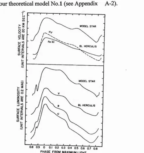
Page-17-Most of the short period (BL Her) Pop II Cepheids show similar light curves in shape. The following characteristics can be seen in most of BL Her light curves, a steep rising branch, a pronounced maximum, a secondary hump or shoulder on the descending branch and a quite large amplitude, (see Appendix A2 and Figure 3 in Kwee 1967 and discussion therein).

1B~3.

W

:-These variables are defined as any cepheids of Pop II with period longer than 3 days. They are the more luminous cepheids and they are identified with stars undergoing blueward loops from the second giant branch in response to He shell flashes or finally evolving to the blue as the H-burning shell near the stellar surface (Gingold 1976).

The W Vir variables - as we have seen - are considered to be the Pop II counterparts of the classical cepheids, see Figure 1-1 and table 1-1. Some of them exhibit RV Tau type behaviour (Clement et al 1988).

These variables are AGB stars that undergo blue loops in response to He-shell

flashes. Models with envelope mass less than 0.22 loop enough to the blue to

reach the instability strip (Clement et al 1988). Depending on the envelope mass, the star may enter the instability strip several times as a result of the adjustments between the two shells - Hydrogen and Helium burning shells - (Gingold 1976). The time spent in the instability strip varies inversely with mass and independently of Y, in the range

Chapter ONE

Page-18-The period range, say from 2-45 days, is roughly the same as for the classical cepheids. Most W Vir variables, however, have periods within the range of 2-20 days. They are high velocity objects and lie at great distances from the galactic plane (more than about 200-300 Parsecs, see for example Strohmeier 1972, Cox 1974) . Many of W Vir are found in globular clusters.

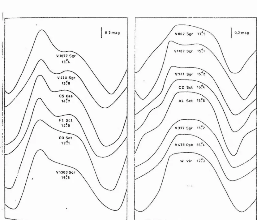
The light curves of the W Vir do not conform to the Hertzsprung relation, but they seem to be characterised by the presence of a shoulder on the descending branch, see Figure 1-6. The total magnitude range is about 1 magnitude, roughly the same as that of classical cepheids.

The radial velocity curves vary, in the same qualitative way as the RR Lyrae. A number of other qualitative similarities within velocity curves and spectral features of the latter kinds of stars suggest that qualitatively similar physical mechanisms are operative in the atmosphere of these two types of stars (Cox 1974).

The W Vir obey a period-luminosity relation, approximately parallel to and about 1,4 magnitude below the classical cepheids P-L relation, see Figure 1-7 (Cox

1974).

W Vir stars originate from a narrow mass range which is about 0.6 + 0.1 _{M sun}

Bumps in the light curves are surely the result of a near resonance between the fundamental mode and the second overtone period (Wallerstein & Cox 1984 ).

Chapter ONE

Page-19-X A 190010 S g r

/ \ l3 4 2 V74I Sgr / \ ^ ^ _ ^ I 7 I 3^ CO S e t

y aO Z S g r AD A ra W Vir / \ ^ 1 3 - 5 1 / \ — . 16 02 y N _ _ ^ 1 7 - 2 7

190018 S g r V478 Oph / X ST Pup

/

V 4I0 S gr

/ X ^ ^ - 7 8 / --- S J 6 -4 4V3B3 S g r / \ X \ TW Cap 2 8 -5 8

Figure 1-6. Light curves o f twelve galactic W Virginis variables with star name and period (in

days) indicated for each curve. Ordinates are apparent magnitude, abscissa are phase (from Cox 1974 fig.

8).

1-4 m Classicot

cepheids

W Virginis variables

RR Lyrae variables

- 0 5 0 0 5 10 15

log TT

Figure 1-7. Empirical period-luminosity relation (schematic) for classical cepheids, W

Chapter ONE

Page-20-The relative radial excursions of W Vir are much larger than those of the classical cepheids. The radius fractional semi-amplitudes are around 0.10 - 0.30, compared to about 0.05 - 0.10 for classical cepheids, (Cox 1974).

Observations, especially of the velocity variations, of W Vir are unfortunately rather scarce. The major observation concerning velocity is that the stars with periods above 13 days have highly asymmetric velocity curves frequently accompanied by H emission lines at rise to maximum light. This is probably caused by strong outward moving shock waves (Bridger 1984).

According to the shape, the light curves of cepheids (W Vir) divide into two major classes, see Figure 1-8 ;

1) Crested "C-type which shows a bump or standstill on descending light rather like the classical cepheids with period 5-10 days , Cox (1985).

2) Flat-top " F-type " sometimes has a bumps on rising light as cepheids with period 1 0 - 2 0 days, Cox (1985). The flat maximum may last for 0.3 in phase, Kwee (1967).

The C- and F- type variables occupy different positions in the H-R diagram. The crested variables are about half a magnitude brighter than the flattened one (Kwee 1968).

Chapter ONE

Page-21-instability previously found to be characteristic for models with He burning shell sets in and causes the characteristic shell flashes (Schwarzschild & Harm 1970). If we make the simple assumption that metallicity varies very little, or that it has little effect on the evolution, then it is possible that a slightly higher mass star moving up the AGB executes this blue-loop at a later stage, causing the star to have a higher luminosity when passing through the instability strip producing a C-type variable (see discussions in section lB-2). Thus we see that the C-type variables may be slightly more massive than the F-type. Assuming the two classes follow the parallel period-radius relation, which is independent of the chemical composition, then the mass ratio may be estimated as giving Mc~1.3M/', where Me and M/^ refer to the crested and flatted masses respectively. This fits into the range of possible masses given by Bohm-Vitense (1974) of 0.5 < M I M _sun < 0.75 (Bridger 1984)._{\ o /}

The width of the instability strip depends on a combination of mass (increasing the mass leading to shift the blue edge to the higher temperature), luminosity (increasing the luminosity leading to shift the red edge to redder colours) and chemical composition. The red edge of the strip defined as the value of 7 ^ at which

the growth rate, 77, is maximum, (fractional amplitude increases per period, where

77 oc ^ ^ ^ ^ surface gravity, Cox (1980) and Chiosi et al (1992)).

The growth rate of W Vir instability is very rapid because of the large luminosity to mass ratio (see for example, Davis 1974, Fadeyev 1993).

Chapter ONE

Page-22-responsible for the existence of the red edge (Wallerstein & Cox 1984, Buchler & Moskalik 1992).

0 2 m ag _{V 802 S g r 1375} 0.2 m ag

v n e ? Scr 1571 V1077 Sgr

13ft

V7t 1 Sgr 1572 V t I O S g r

13?8

V377

V 478

V 1303 S g r 18?5

CHAPTER

Chapter TWO

Page-24-2‘L

:-Here we will mention only the non-linear approach since the linear theory is expected not to be an accurate account for the location and width of the H-R diagram, (Christy 1966, Cox 1974). The linear theory, for the sake of completeness, is briefly discussed in Appendix D.

2-1-L

Chapter TWO

Page-25-The pulsation constant Q characterise the pulsation mode of a star, and is defined as :

Q=P,

sun

where

P

Q

The gamma effect arises from the variation in ratio of the specific heat of the gas during ionisation. If the gas in the pulsation driving layers is compressed, much of the work done on this layer is used to ionise the gas and only a small part is used to raise its temperature. During a later part of a pulsation cycle, when the gas is expanding the ionisation energy is recovered with recombination occurring the phasing of this re-emergence of energy is delayed a bit so that it actually reinforce the expansion (Keeley 1970, Wallerstein & Cox 1984).

The kappa effect, which causes a strong driving of the pulsation in the region outside the H ionisation zone, is a material property that causes destabilization of stars. In this case the energy is not hidden for part of a cycle, but it is merely blocked by the higher opacity. Energy is allowed to flow more easily during expansion, and this gives the re-expansion a push. (Keeley 1970, Wallerstein & Cox 1984).

Chapter TWO

Page-26-is set by the abundance of He. This is because, for the hotter stars, H ionisation driving is too near the stellar surface (Wallerstein & Cox 1984).

2 -2 Th e Eotjattons Of St e l l a r Pu l sa t io n

:-In modelling pulsating stars we have to set three assumptions which are as follows;

(1) space is Euclidean ,i.e. flat space. (2) mass is conserved.

(3) Newtonian theory expresses the gravitation; neglect the effect of special and general relativity.

2 -2 -2 Th e Ba sic Eo u a t iq n s

Chapter TWO

Page-27-The mass continuity:

â r

1

à

A f 4;r

The hydrodynamic equation (equation of motion):

â ^ r _ _ GMr _

â P

(2-2)

--- (2-3)

à f

r

â M ,

Most stars are obviously in such long-lasting phases of their evolution that no changes can be observed at all. Then the stellar matter cannot be accelerated noticeably, which means that all forces acting on a given mass element of the star compensate each

other. In these cases we have the hydrostatic equilibrium when, — is equal to

à f

zero.

The equations of mass continuity - (conservation of mass) equation 2-2 - and that of momentum - (equation of motion) equation 2-3 - determine the dynamical behaviour of the stellar envelope (Unno 1965).

The radiative energy transfer:

' r

(In some textbooks they use (2 x C rather than 4 O' )

where:

T : space variable (radius).

t : time variable.

M r : mass enclosed within radius r. P : density of matter at radius r.

Chapter TWO

Page-28-Lr

r.

P

T

r.

r.

CJ : the Stefan-Boltzmann constant.

(I : the radiation pressure constant = 7.56 x 10"'^ erg cnf^ K .

The conservation of energy equation ^ :

= S

<

.,,

â t

Ô t

An r - p â r â t

where,

E

V

Q

The alternative form of energy conservation is

^ We can write the energy equation as 1

d t a t â Mr

•1

where S and Q are the entropy and the specific heat respectively. First low o f thermodynamics gives us |

!

\F . = Q — W , where W=^PdV the work done, |

!

a E a L ^ a V 3

so , = - ---P---+ g v|

a t a M y a t \

Chapter TWO

Page-29-( # r - r P ^ L ) = 0

(2-6)

These equations - along with formula for opacity, energy generation and equation of state and suitable boundary conditions - can be solved for the radial pulsation. Practical difficulties remains in the inclusion of convection in pulsation calculation. Convection means an exchange of energy between hotter and cooler layers in

= P — 4/r r"

_ p — ~ P

Chapter TWO

Page-30-a dynPage-30-amicPage-30-ally unstPage-30-able region through the exchPage-30-ange of mPage-30-acroscopic mPage-30-ass elements, the hotter of which move upwards while the cooler ones downward. The moving mass element will finally dissolve in their new surroundings and thereby deliver their excess - or deficiency - of heat. Owing to the high density in stellar interiors, convective transport can be very efficient. However, this energy transfer can operate only if it finds a sufficient driving mechanism in the form of the buoyancy forces. Convection and pulsation tend to be mutually destructive phenomena. Rapid thermal alterations arising from pulsation may tend to prevent convection from becoming firmly established, while convection may conspires to quench pulsation by altering the thermal structure of the H ionisation region in a certain manner. This would imply that convection is relatively unimportant except when close to the red edge ( i.e. convection is able to quench the pulsation at relatively low pulsation amplitudes). By ignoring the convection the light and velocity curves are relatively unchanged (Christy 1966, Clayton 1968, Deupree 1977a, b, Buchler 1990). Neglect also of rotation and magnetic fields means that the only forces acting on a mass element come from pressure and gravity. We also assume that the diffiision approximation for energy transfer by radiation holds throughout (Christy 1967, Clayton 1968, Strohmeier 1972, Stellingwerf 1975, Bridger 1983, Kippenhahn & Weigert 1990).

It is assumed that only the stellar envelope takes part of the pulsation, where there is no energy generation, and where we must include a realistic opacity law and an equation of state that includes ionisation, since these properties are basic to the existence of pulsation instability. For most problems, the central core of the star can be ignored. We believe that this region plays very little part in the pulsation.

Chapter TWO Page31

-energy generation on the right hand side of the heat flow equation, (see for example, Christy 1967, Bridger 1983 and Milligan 1989). Thus:

â E ^ p â V _ _ _ _ _ Ô L _ _ â L

Ô t ô t ^ T t r ^ p â r p M

2-2-2.

:-The inner boundary is chosen such that the radius of the innermost zone in the pulsation calculation is fixed at its equilibrium value which is

R

Thus, only the stellar envelope participates in the pulsation, this means that the luminosity and composition are constant in the initial model (Christy 1967, Bridger 1983), since the core is assumed to be non-pulsating while radiating a constant luminosity. Thus, at the inner radius

and

(2- 10)

inner

At the inner boundary the velocity is zero at all times and the luminosity is a constant (i.e. the core luminosity).

At the surface of the star we can see two boundary conditions, either:

jP{tot-surface) ~ P{vad-surface) (2-1 1)

Chapter TWO

Page-32-P (tot—surface) ^ (2-12)

Dr, Carson used the second one in his program, where

P{tot) the total pressure.

PfPQ^ is the radiation pressure which should be described by the time-dependent radiative transport equation. This is not possible, because it requires knowledge of the state of gridpoints several mean free path lengths away. Therefore, the radiative boundary condition is chosen to approximate the results of diffusion theory. The radiation pressure is important only at high temperatures (Clayton 1968, Milligan 1989). By using the Eddington approximation^, this can be expressed as

( D 1

= I

' = I

'

T e ff ’ effective temperature. 'J'^ ; surface temperature.

T ; optical depth.

^The Eddington or simply the T-x approximation is defined as follows

4 3 4

CHAPTER

Chapter THREE

Page-34-3-1.

:-Equations 2-2, 2-3, 2-4 and 2-7 are treated as an initial value problem, to be integrated from initial conditions. In order to follow the non-linear behaviour of the model, it is necessary to put these equations in difference form, in a stellar envelope of about 50 mass zones. This procedure is described in Christy (1967). In our work, we will follow the same procedure as Milligan did in her Ph.D. thesis (1989), We will use a program written by Dr T. R. Carson. Some of the main features of this program are given here for the sake of completeness.

Chapter THREE

Page-35-The boundary between each zone is labelled i, where i = 1 is the innermost zone, and i = N the outermost. The centre of each zone is labelled i - Yz. The radius is taken at the boundary. Therefore, would be the radius of boundary i at time f , where n specifies the time-step. The mass of the zone, A ]\/[. _y ,and the mass at the boundary, A , are both useful quantities and are defined as follows:

A M i -1^ = M r M i -1 ; mass of the zone (3-1)

A M , = ^ (A M , - ) 4 + A M , boundary (3-2)

and the specific volume V of the zone :

j r . _ 4 ^ ( Æ " y

-The re-zoned model extends inwards to about 0.1 - outside nuclear energy producing region, where luminosity is constant and has a small amplitude of pulsation. We have now relaxed this envelope onto the same difference equations as used in the pulsation analysis, otherwise problems would arise in the pulsation calculations. The relaxation is achieved by an iterative scheme, which calculates y and

from the outer boundary condition, then, for all W - 1 zones, it calculates p . _y

Chapter THREE

Page-36-Velocity U is taken at time « + V2 for best centring in time. Thus, the radius at

the new time w + 1 is given by:

R7' = r :

(

3

-

4

)

where:

p;*'A = u '^ 'A (3.5)

= r ' “ f (3-6)

A f -

r

where At"*^ is not necessarily the same as At". The program changes the time-step as it process, in order to facilitate convergence. The first time step is usually the most stringent, so the time-step must be less than the time for sound to traverse any zone (Bridger 1983). Therefore,

'■/l T

A M < (3-8)

where the square root is of the order of the mean velocity of sound on the stellar interior.

During the pulsation a shock wave develops, which can cause a rapid compression (but not an expansion), of some zones particularly in the H ionisation region. Therefore, we have to add an artificial viscosity pressure, which acts as an extra pressure which enabling the shock front to be spread over several zones, thus,

improving the stability. A large Cq makes a thicker shock front but greater stability

Chapter THREE

Page-37-= C g

[M m

( ^

^

+ y ,0)] '

(w,

where superscripts refer to time and subscripts to zone, and l |/ is of the order of 0.1.

Stellingwerf (1975) found that when \j/ = 0 we get a damping in the lower region of the envelope. As \ |/ gets larger the time steps gets bigger and the amplitudes are up to 50% higher than those indicated by the observation (Kovacs 1990).

We can now write the equation of pulsation in difference form, and consider the boundary condition on them. The equation of hydrodynamic equilibrium, 2-3 , can be written as:

(

:

a m

(3-10) The boundary value of this is as follow:

Inner:

= 0 (3-11)

Chapter THREE

Page-38-- A f {

GM «

( R

)

(

: y

A M

(3-12) where V P is \ The expression for the outer boundary condition is obtained by

defining some fictitious pressure, ^ , beyond the outer surface of the star.

For a zero surface gas pressure we have:

(3-13)

(3-14)

P r Fn-y = \^W r-yrP .-y

since the atmosphere is almost isothermal. Then we can write with a good approximation (about 1% Bridger 1983)

P ^ , = i a f K - y , (3-16)

where is the radiation pressure at the surface.

Bridger also adopted mass zones increasing inwards by a constant factor OC (the Carson non-linear code which has been adopted -as mentioned earlier- incorporating mass zones of equal sound travel). Hence for consistency he used

1+OC

— — A M at-K (3-17)

Chapter THREE Page-3

9-where,

A M k = I ( A M n.K + ) (3-19)

The radiative energy transfer equation, 2-4, becomes:

z

;=[

47

i

(

r i

Y

]

[ w i y - w i J ^ F :

0

-

20

)

where 2 is a suitable difference form of y Y ^ ■

Then:

« _ 4 (7 1

3

M,..y+K

i-y,^ M,-y

^ ^

Christy (1967) found that using this relation in the iteration of the heat equation failed to converge when the front was advancing outward with large amplitude. This is because this relation can not handle the large change in opacity across a zone that occurs in such cases. It gives too little weight to the larger opacity, that means , to minimise the error produced by the use of very coarse zoning in the region of H ionisation (Castor 1971, Bridger 1983). Therefore Christy developed a new difference expression for F. Thus:

3

K.'Lu

(3-22)

is thG opacity in at i + Yz.

Chapter THREE

Page-40-(

piy+F:,)+QZIvTrrvlyy^

—

^ r

T-H+ii r __ r«+i_ r

1

J

(3-23)

This is solved at each time step, by a process of iteration, which is subject to the inner and outer boundary conditions. Since no energy generation takes place in the pulsation envelope (i.e. the energy generation equal to zero). The inner boundary conditions imply that the luminosity of the innermost zone is equal to the total

luminosity of the model. Thus at i = 1 we can determine ,thus k

z r - [ 4 7 i 0 -24)

where is the mean luminosity.

The outer boundary condition makes use of the Eddington approximation. The surface luminosity is given by:

d—M. = 4Ti r^p d r

L = -(47t r ' ) ' [ i ^ | E ] = -(4 n / )' [aw ]2F

let, =

SO, L = (4nr^ Ÿ H = (4 n r^Ÿ A W 2 F .*. flwc= , ^ j = (4ti )H

Chapter THREE Page41

-L = A

{ R ^ S

2 a T ,

Therefore we have to determine , which is the radius at which the temperature is equal to the effective temperature, . Bridger (1983) found that and 7?jv-i i^ight be unreliable in some model. Now we can write down the outer boundary condition:

{ E

t y r E 'ly + [l, { P l y + F ;\) + Q t y J V t y r V l y ^ ^ M .-y

= ^ t e . + z ; - - 2 ct 4% W s - y + i R Z T m i y ] }

(3-26)

Equation 3-23 can now be solved for new temperature by using a

Newton-Raphson iteration method. Thus we can do by making a linear expansion of the various terms in the difference equations and solve each step of the iteration procedure. Let a superscript prefix denote the number of the iteration, and let ^ t>e the correction to the temperature at each iteration i:

then we have:

• pi j-tH+1

" F l y =

'ET

+

^ fr/+X _■I

Chapter THREE

Page-42-" C

(R'r'ŸÎ {w":yrWi:'^^FT'

(3-31)

When equations 3-27 to 3-31 are substituted into the difference form of the energy equation, 3-23 , we get:

a . K ‘a^ : ; = ô. k

where:

a . x = ^ r ^ [ x . f { w. : y r (3-3 3)

^ W ,.y

(3-34)

(3-35)

5 , .x = - r : : - L : ] - ^ M , . y { E T y - E i y

+ [ | ( p . x + 'p : ':

U + a : x l L : ; - F : 'J }

(3-36)

1

Chapter THREE

Page-43-X ' = 4 7 l ( i ? r ) (3-37)

Equation 3-32 is a matrix equation of the form M X = D, where M is a tridiagonal matrix with elements Ot , P and y , X is the solution matrix containing

new values of and D is a column matrix with elements Ô. The equation can

be solved using a standard technique.

Equations 3-33 to 3-37 provide most of the elements of matrix M. The boundary conditions give the following values for the remaining elements:

• ^ M-bl ■ •

a y = 2(A rY ( f : ' -

[ V ;'-V k ']}

(3-3»)

O Wy,

• /I4-1 • ^

p =

2

( x ' ) ' { V r + — ^ V ; ‘-

W y ] }

(3-39)

d Wy

y = 0

Ô K =2 ( x ‘) ' { V r ' [ V ; ' - (3 -« )

= 0 (3-42)

o N-y^

Chapter THREE

Page-44-- " d w . -_K

(3-44)

0.-^=^ [ z ; - . + ‘z :',- 2 a

(

a"^,,W",-A AZ.WT-y)]~

a

M .-y

{ z r K - p ; - K + R (F . - K + > ; - K ) + c y

(3-45)

To solve the matrix, we look for two sets of equations Xl^.y and Yn.y such that

^ f v : : ÿ = x , . y ^ p r ; : ÿ + r . y (3-46)

then

^ W : y = X . - y ^ W : : y + Y ,-y (3-47)

Substituting 3-47 into 3-32 and dropping time superscripts, we get:

-K ^

So we obtain:

(Xi+/2

and

Î

Chapter THREE

Page-45-_

P(+x y

Y , . y =

n

So starting at i =1 , all of X/+j^ and Yi+y^ can be calculated from 3-49 and

3-50. At the surface ~ 0 , i.e. Xs-y^ is zero, therefor,

W . - y = Y .- y (3-Sl)

SO all the can be found from 3-48. Iteration proceeds until the temperature

correction terms are as small as is desired.

3-2.

:-In order to solve the stellar structure equations it is necessary to have an equation expressing the relation between

P, T

S,

E,

Let A., be the atomic mass of element i, be the abundance by mass of element i, CL. be the abundance by number of element i, and |Ll be the mean

molecular weight, thus:

Chapter THREE

Page-46-P .

A,

i=l

Z

P ,/

/ A i

The quantity N may not be known, depending on whether the pressure or

density is known. If P is known then

N ~P !KT

N = N - N

Pçr

P

N

N

^ A o _ £ O L i (3.54)

where:

JV^ is Avogadro's number, and K is Boltzmann constant.

If we let

iV..

V ^

be the electron density. Then, the electron number density is given by:

all all

N e = Y . l . j (3-55)

y=i

This expression is non-linear in which can be solved by iteration.

Chapter THREE

Page-47-P=P.

+ P + P

where :

the radiation pressure is

P =-aT ^

,

3

the electron pressure is

P = N K T ,

the ion pressure is

P. = N K T

;the electron number density

;the nuclei number density

N

N - N 4 -N

The prefix Hon' denotes the contribution from free ions which remains to be calculated.

To find the number density N ^j of element i in ionisation state j, we can use

; 'ki

Chapter THREE

Page-48-N

n V .® ,/

D

N ol!

..'i-'

' z [ n w 7 ) ]

/ = 1 J = ( Ù j

in which we have:

(3-61)

(3-62)

& !

where,

; the highest ionisation state of element i .

P _ ; the partition function for the ionic species(ÿ)*

g .. ; the statistical weight of the outer shell. U

V.. ; the number of electrons in the outermost shell.

; the ionisation energy. j

h : the Planck constant. i

1

jfl ;the electron mass. |

Chapter THREE

Page-49-all

e - « > i- i I

the partial entropy per unit mass is:

^ion " ^ ^ ~ ^ io n . ^ i o n . ^ T ] (3-65)

and the partial internal energy per unit mass is:

1 all *^7 ^ Q

£ , = p [ z ( 3 ^

^ i~l j=(ûf ^

the total energy per unit volume is given by

E=E.

+ c

T ^

a f -,

c = —N K

(3-68)

V 2 "

then;

E = E. + - N KT+aT

2 ^

TS = P+U+r[KT

Chapter THREE

Page-50-g / = W [2 ; r A . K T i h Z - (3-7i)

The equation of state also allow for the formation of the molecules and

C O , being the most abundant of the diatomic molecules. For these the abundances are readily obtained by the solution of quadratic equations since the equilibria are not coupled. The expression for the pressure and stellar thermodynamic properties are then suitably modified.

Some references that were useful here are; Christy 1967, Clayton 1968, Cox & Giuli 1968, Copeland et aL 1970, Bowers & Deeming 1984 , Bridger 1983 and Milligan

Chapter FOUR

Page-52-4-1,

In this work, as mentioned earlier, we have used a program code written by Dr. T. R. Carson. The input data were as follows: the star's mass, luminosity, effective temperature or radius, the hydrogen content X, helium content Y and metal content Z and number of the zones required. The results are shown in table 4-1. We have used the Iglesias and Rogers opacity tables which have been modified by Dr. Carson to include molecular opacity of lowest temperature. This work has been done using the SUN computer system at the University of St. Andrews.

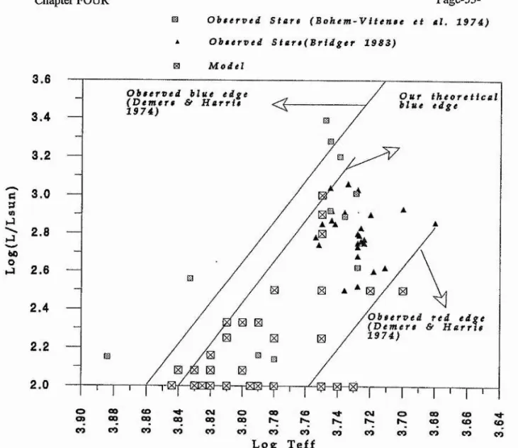
In our work we have used the same parameters that were used by CS82 & CSV81 (models 1 - 20), three models from Bridger 1983 (models 31, 32 and 34), five models from Hubickyj 1983 (models 35 - 39), and the other models have been adopted by the author. Figure 4-1 shows our models in HR diagram, the observed stars - using table 1 in Bohm-Vitense et al 1974 and tables 2-la and b in Bridger 1983 -. Also shown the observed blue and red edges, equations 4-1 and 4-2 respecivly, which have been adopted from Demers & Harris 1974 (these edges only for BL Her and W Vir stars).

lo;s(7:/Z,,un) = -10/75 lojg k43.5 O#-!)

loi,(jL/ I,un) = --10.75 lois 2:# -^4:2.4 (.4-2)

Chapter FOUR Page-53-O bt e r v è d S t a r s ( B o h e m - V i t e n s e e t al. 1 9 7 4 )

O b s e r v e d S t a r s ( B r i d g e r 1 9 8 3 ) M o d e l

3.6

O b s e r v e d blue edge ( D e m e r s & H a r r i s

1 9 7 4 ) O u r t h e o r e t i c a lbl ue edge

3 .4

3.2

bO O

2 .4

O b s e r v e d r e d e d g e ( D e m e r s & H a r r i s 1 9 7 4 )

2.2

2.0

0 0 0 < O ^ C 4 0 a o < 0 ' ^ C N J

c » o o o o Q O Q O Q o r « . r ^ i s . , r ^

c o c o c o c o n o c o c o c o c o

o

r». CO CO

CD CO

L o g T e f f

Figure 4-1. Shows the observed stars, blue edge and red edge, and theoretical blue edge and models.

CO

CO CO CO CO

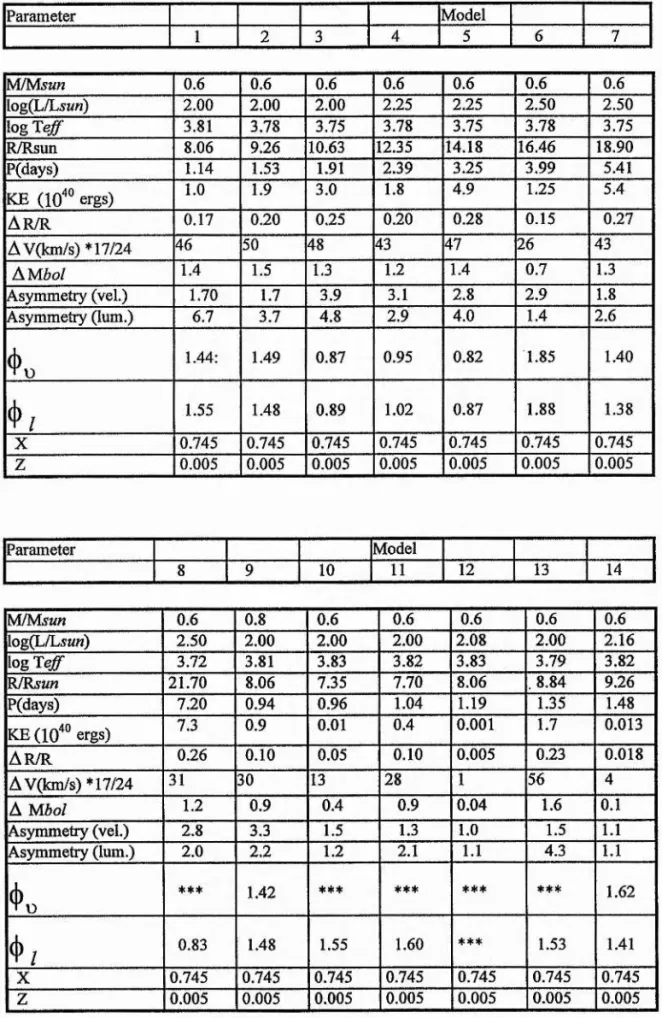
The main results are summarised in table 4-1 which contains the following;

KE ; peak kinetic energy.

A ; full amplitude.

Asymmetry ; time spent on the descending branch of the surface velocity curve (or surface luminosity curve) divided by time spent on the ascending branch.

(j) ; phase after zero velocity on the ascending branch of the surface velocity

curve of the second (not necessarily the secondary) bump on this curve plus unity.

(j)^ ; phase after mean bolometric magnitude on the ascending branch of the

Chapter FOUR

Page-54-Table 4-1. Shows a summary of our models' results.

Parameter Model

1 2 3 4 5 6 7

M/Msun 0.6 0.6 0.6 0.6 0.6 0,6 0.6

log(L/Ljw«) 2.00 2.00 2.00 2.25 2.25 2.50 2.50

log Teff 3.81 3,78 3.75 3.78 3.75 3.78 3.75

R/Rsun 8.06 9.26 10.63 12.35 14.18 16.46 18.90

P(days) 1.14 1.53 1.91 2.39 3.25 3.99 5.41

KE (10^® ergs) 1.0 1.9 3.0 1.8 4.9 1.25 5.4

Ar/r 0.17 0.20 0.25 0.20 0.28 0.15 0.27

AV(km/s) *17/24 46 50 48 43 47 26 43

A M bol 1,4 1.5 1.3 1.2 1.4 0.7 1.3

Asymmetry (vel.) 1.70 1.7 3.9 3.1 2.8 2.9 1.8

Asymmetry (lum.) 6.7 3.7 4.8 2.9 4.0 1.4 2.6

1.44: 1.49 0.87 0.95 0.82 1.85 1.40

1.55 1.48 0.89 1.02 0.87 1.88 1.38

X 0.745 0.745 0.745 0.745 0.745 0.745 0.745

z 0.005 0.005 0.005 0.005 0.005 0.005 0.005

Parameter Model

8 9 10 11 12 13 14

M/Msun 0.6 0.8 0.6 0.6 0.6 0.6 0.6

\og(L/Lsun) 2.50 2.00 2.00 2.00 2.08 2.00 2.16

log Teff 3.72 3.81 3.83 3.82 3.83 3.79 3.82

R/Rsun 21.70 8.06 7.35 7.70 8.06 .8.84 9.26

P(days) 7.20 0.94 0.96 1.04 1.19 1.35 1.48

KE(10^® ergs) 7.3 0.9 0.01 0.4 0.001 1.7 0.013

Ar/r 0.26 0.10 0.05 0.10 0.005 0.23 0.018

AV(km/s) *17/24 31 30 13 28 1 56 4

A Mbol 1.2 0.9 0.4 0.9 0.04 1.6 0.1

Asymmetry (vel.) 2.8 3.3 1.5 1.3 1.0 1.5 1.1

Asymmetry (lum.) 2.0 2.2 1.2 2.1 1.1 4.3 1.1

4 ) . *** 1.42 *** *** *** *** 1.62

0.83 1.48 1.55 1.60 *** 1.53 1.41

X 0.745 0.745 0.745 0.745 0.745 0.745 0.745