A superresolution land cover change detection method using remotely sensed images with different spatial resolutions

A Super-Resolution Land-Cover Change Detection Method Using

Remotely Sensed Images with Different Spatial Resolutions

Xiaodong Li, Feng Ling, Giles M. Foody, IEEE Fellow, and Yun Du

X. Li, F. Ling and Y. Du are with the Key laboratory of Monitoring and Estimate for

Environment and Disaster of Hubei province, Institute of Geodesy and Geophysics,

Chinese Academy of Sciences, Wuhan 430077, PR China (e-mail:

[email protected]). G. M. Foody is with School of Geography, University of

Nottingham, University Park, Nottingham NG7 2RD, U. K.

Abstract—The development of remote sensing has enabled the acquisition of information on land-cover change at different spatial scales. However, a trade-off

between spatial and temporal resolutions normally exists. Fine-spatial-resolution

images have low temporal resolutions, whereas coarse spatial resolution images have

high temporal repetition rates. A novel super-resolution change detection method

(SRCD) is proposed to detect land-cover changes at both fine spatial and temporal

resolutions with the use of a coarse-resolution image and a fine-resolution land-cover

map acquired at different times. SRCD is an iterative method that involves

endmember estimation, spectral unmixing, land-cover fraction change detection, and

super-resolution land-cover mapping. Both the land-cover change/no-change map and

from–to change map at fine spatial resolution can be generated by SRCD. In this

study, SRCD was applied to synthetic multispectral image, Moderate-Resolution

Imaging Spectroradiometer (MODIS) multispectral image and Landsat-8 Operational

Land Imager (OLI) multispectral image. The land-cover from–to change maps are

found to have the highest overall accuracy (higher than 85%) in all the three

experiments. Most of the changed land-cover patches, which were larger than the

coarse-resolution pixel, were correctly detected.

I. I

The detection of Earth’s surface change serves as the basis for global change

studies, and is critical to the understanding of the interactions between human and

environmental systems. Remotely sensed data have become a primary data source for

monitoring land use/cover distribution and its changes at different scales [1]. At the

global scale, the coarse (low) spatial resolution images are the main data for

land-cover monitoring. For instance, land-cover change products based on MODIS

images at annual steps and 500 m spatial resolution for 2001-present have been used

for global monitoring and assessment purposes. Coarse spatial resolution remote

sensing systems have typically a high temporal repetition rate, which allow the timely

detection of land-cover changes. For example, MODIS allows the entire surface of the

earth to be monitored every 1 to 2 days since 2002. However, because of the relatively

coarse spatial resolution of the images acquired the level of spatial detail detected is

low. At the local-regional scale, land-cover change is often detected with the use of

fine (high) spatial resolution remotely sensed images, such as those acquired by the

Landsat Thematic Mapper (TM), Landsat Enhanced Thematic Mapper Plus (ETM+),

and Systeme Pour l'Observation de la Terre (SPOT) sensors. However, owing to the

trade-off between spatial and temporal resolution, fine-resolution images are often

acquired at a relatively low temporal resolution. Thus regional land-cover change

products are typically updated infrequently. For instance, the National Land Cover

Database (NLCD) land-cover change product for the U.S.A. with a spatial resolution

of 30 m is updated every 5 years approximately. Furthermore, fine-resolution images

usually cover a relatively small area, making their use difficult for regional or global

land-cover monitoring due to the great amount of processing time and labor required.

The accurate and timely detection of land-surface changes is a challenging task.

Land-cover change detection is crucial to understand and quantify land-cover change,

which is increasingly recognized as an important driver of global environmental

change [2]. The most widely used land-cover change detection methods are

methods, such as image differencing [3], vegetation index differencing [4], and

change vector analysis [5]. However, these change detection methods are based on

per-pixel comparison and require the same spatial resolution for bi-temporal images.

Different resolution images are usually resampled during the spectral change

detection process. A problem occurs when spectral modalities are different, and

simple change detection (e.g., image differencing and thresholding) is often unreliable

or impossible in case channels do not overlap well in the spectral ranges. Medium- or

fine-resolution images are the main data sources for change detection; however, they

are acquired at low temporal repetition rates, and land-cover changes are detected

infrequently. By contrast, coarse-resolution images, which have high temporal

repetition rates, are the main data sources of land-cover change detection at a global

scale. Unfortunately, the aforementioned per-pixel-based change detection methods

assume homogeneity within a single pixel, resulting in no quantifiable changes at the

sub-pixel level. In fact, most coarse-resolution image pixels are composed of several

land-cover/land-use types, and the mixed pixel problem seriously affects the change

detection accuracy. Spectral unmixing or soft classification algorithms do not assign a

mixed pixel to a single land-cover class but instead generate class area proportion or

fraction images that represent proportional areas of different land-cover classes within

mixed pixels. Spectral mixture analysis can be used to derive land-cover area

proportion images, and changes can be detected by comparing the “before” and “after”

area proportion images of each endmember[6]. Applying spectral unmixing to

bi-temporal or a series of multitemporal images for change detection can potentially

reveal important sub-pixel level information, such as the endmember abundance

variation in a given location [7-10]. Spectral unmixing-based change detection

methods provide the addition/subtraction of an endmember in the abundances and are

based on the images with the same spatial resolution. In addition, He´garat-Mascle et

al. [11] used images with different spatial resolutions to detect sub-pixel land-cover

proportional change. A coarse-resolution image was unmixed and a fine-resolution

image was spatially degraded to generate the bi-temporal class area proportion images.

change in the class proportions of each coarse-resolution pixel was detected. However,

only the coarse-resolution pixel change instead of the fine-resolution pixel change

was detected, because spectral unmixing can only determine the coarse-resolution

pixel land-cover area proportions and does not provide information on class labels at a

sub-pixel scale.

Super-resolution land-cover mapping (SRM) is a technique used to generate

land-cover maps with a finer spatial resolution than the input data. Various algorithms,

such as pixel swapping algorithm [12, 13], Hopfield neural networks-based SRM [14],

Markov-random-field-based SRM [15, 16], the spatial-spectral managed SRM [17,

18], spatial interpolation based SRM [19, 20], direct mapping based SRM [21],

example-based SRM [22] and intelligence system based SRM [23], have been

proposed to address the SRM problem. SRM predicts the spatial distribution of each

class in each coarse-resolution pixel and provides more sub-pixel-scale land-cover

information than spectral unmixing[24]. Traditionally, SRM is applied to a

monotemporal coarse-resolution image to predict a fine-resolution land-cover map for

the time period it represents. SRM is an ill-posed inverse problem because many

fine-resolution land-cover maps can satisfy the SRM constraints, and traditional

methods using a single image are limited in terms of the spatial detail represented and

the accuracy of the final map produced. Additional datasets can, therefore, be adopted

in SRM. A historic fine-resolution land-cover map may, for example, be used to

enhance SRM. Ling et al. [25] first proposed a sub-pixel land-cover change mapping

method by integrating a coarse-resolution image and a fine-resolution land-cover map

that pre-dates the former. In this method, the sub-pixel class labels in the

fine-resolution map with unchanged or increased class area proportions are preserved

in the final fine-resolution land-cover map output from the SRM, and other sub-pixels

are allocated based on the land-cover maximum spatial dependence model. Li et al.

[26] proposed a spatial-temporal Markov-random-field-based SRM, in which the data

on land-cover temporal dependence is the input to the analysis. Xu and Huang [27]

proposed a spatial-temporal pixel-swapping algorithm based SRM, which extended

et al. [28] proposed a spatial-temporal Hopfield neural network based SRM, in which

temporal transition information of sub-pixels was added compared with traditional

Hopfield neural network based SRM.

Although the capability of SRM to extract fine-resolution land-cover information

is increased with the use of a fine-resolution land-cover map that pre-dates the

coarse-resolution image, the existing methods have three major limitations in the

detection of land-cover change at fine spatial and temporal scales:

(1) With current SRM methods, the required information on endmembers, which

can represent the spectral information of land-cover components, is typically assumed

available. However, endmember information is often unavailable; thus, the extraction

of endmembers in SRM is necessitated. Endmembers represent the spectrally pure

components of a given image and are central to SRM. A considerable number of

image endmember extraction algorithms, including the manual endmember selection

tool [29], pixel purity index [30], N-FINDR [31], and automatic methods [32, 33],

have been proposed in the recent years [34]. Manual endmember extraction methods

are laborious, whereas iterative and automatic endmember extraction methods have

been analyzed using only monotemporal imagery. When a fine-resolution land-cover

map that pre-dates or post-dates the coarse-resolution image is available, useful

information about land-cover configurations at a former or later time is available to

facilitate SRM analysis.

(2) Current methods consider only the case wherein the fine-resolution

land-cover map pre-dates the coarse-resolution image. Coarse-resolution remotely

sensed images have been available for decades, particularly from such systems as

MODIS and NOAA Advanced Very High Resolution Radiometer. With the

development of remote sensing technology, remote-sensing systems with enhanced

(finer) spatial resolution are increasing in number. As such, the fine-resolution images

that post-date their corresponding coarse-resolution images may often be available in

land-cover monitoring. However, this scenario has not been studied for current SRM

methods.

predicted by SRM, land-cover change information is not provided. Map-to-map

methods demonstrate a potential in fine-resolution change detection using images of

different spatial resolutions, owing to the capability of SRM to generate land-cover

map of a spatial resolution finer than that of the input image. Land-cover change

information can be derived by comparing the land-cover maps of the same fine spatial

resolution; these land-cover maps are generated from fine-resolution images based on

hard classification and from coarse-resolution images based on SRM. This change

detection method provides land-cover change information and trajectories that users

typically desire, particularly a simple binary change/no-change map and the detailed

from–to change trajectory information [6].

In order to address the above issues, a super-resolution change detection method

(SRCD) is proposed. SRCD uses a combination of a fine-resolution land-cover map

and a coarse-resolution image to detect land-cover change/no-change information and

from–to information at fine spatial and temporal resolutions. The fine-resolution

land-cover map can either pre-date or post-date the coarse-resolution image. The

proposed method is based on the assumption that the land-cover class types are

invariant during the period [35, 36]. The endmembers are estimated and iteratively

updated in SRCD. The remainder of this paper is organized as follows. Section II

introduces the SRCD method. Section III examines the performance of SRCD using

synthetic, MODIS, and Landsat images as well as for scenarios in which the

fine-resolution land-cover map pre-dates and post-dates coarse-resolution image.

Section IV concludes this paper.

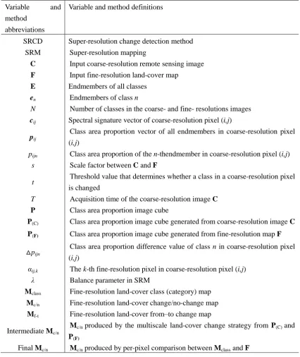
TABLE I.

LIST OF IMPORTANT VARIABLES AND METHOD DEFINITIONS

Variable and

method abbreviations

Variable and method definitions

SRCD Super-resolution change detection method

SRM Super-resolution mapping

C Input coarse-resolution remote sensing image

F Input fine-resolution land-cover map

E Endmembers of all classes

en Endmembers of class n

N Number of classes in the coarse- and fine- resolutions images

cij Spectral signature vector of coarse-resolution pixel (i,j)

pij

Class area proportion vector of all endmembers in coarse-resolution pixel (i,j)

pijn Class area proportion of the n-thendmember in coarse-resolution pixel (i,j)

s Scale factor between C and F

t Threshold value that determines whether a class in a coarse-resolution pixel

is changed

T Acquisition time of the coarse-resolution image C

P Class area proportion image cube

P(C) Class area proportion image cube generated from coarse-resolution image C

P(F) Class area proportion image cube generated from fine-resolution map F

△pijn

Class area proportion difference value of class n in coarse-resolution pixel (i,j)

αij,k The k-th fine-resolution pixel in coarse-resolution pixel (i,j)

λ Balance parameter in SRM

Mclass Fine-resolution land-cover class (category) map

Mc/n Fine-resolution land-cover change/no-change map

Mf-t Fine-resolution land-cover from–to change map

Intermediate Mc/n

Mc/n produced by the multiscale land-cover change strategy from P(C) and

P(F)

Final Mc/n Mc/n produced by per-pixel comparison between Mclass and F

A. SRCD Description

with I × s × J × s pixels with N land-cover classes in it. F can either pre-date or post-date C. The scale factor between F and C is denoted by s, and each coarse-resolution pixel contains s × s fine-resolution pixels. Let Mclass be the fine-resolution land-cover map with I × s × J × s pixels produced by SRM. Endmember matrix E is a B × N matrix, in which each column vector en corresponds

to the spectrum vector of the n-th endmember. Let P be an I × J × N array denoting the class area proportion cube. The N × 1 vector representing the class area proportion of all endmembers in the pixel (i,j) is denoted by pij, and pijn is the area proportion of

the n-th endmember in the pixel (i,j).

SRCD uses a coarse-resolution remotely sensed image C at acquisition time T and a fine-resolution land-cover map F as inputs. SRCD outputs a fine-resolution land-cover change/no-change map Mc/n and a fine-resolution from–to change map

Mf-t. Both Mc/n and Mf-t are produced by comparing F with the estimated fine-resolution land-cover map Mclass at time T.

Central to the proposed SRCD method is the estimation of Mclass from C. Mclass and the endmember matrix E are the two interactive variables in SRCD. If E is known,

Mclass can be produced from C using SRM [25]. Frequently, E is an unknown variable and is estimated from C, given the land-cover area proportion image cube P with the

use of spectral unmixing [11, 37]. P can be derived by spatially degrading Mclass, which is also an unknown variable in SRCD and is iteratively estimated and updated

by determining E [11]. An iterative approach is used in SRCD to solve the endmember matrix E and fine-resolution land-cover map Mclass coupling problem, that is, both variables E and Mclass are estimated and updated iteratively.

The iterative SRCD starts from the estimation of the endmember matrix E at time T. At the first iteration, F, which pre-dates or post-dates C, is used as a substitute of Mclass at time T, which would be accurate if all fine-resolution pixels are unchanged in the time period covered. At each iteration, the estimation of E is solved using a pseudo-inverse method, which employs C and Mclass as inputs. Once E is estimated,

are re-estimated and updated with each iteration. SRCD is iteratively run until

convergence is achieved. Once SRCD converges, Mclass is compared with the input F to produce the final land-cover change/no-change map Mc/n and from–to change map

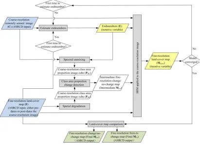
Mf-t. The flowchart of SRCD is shown in Fig. 1.

Fig. 1. The flowchart of the proposed SRCD method.

B. Endmember Matrix E Estimation

In SRCD, the endmember matrix E is estimated based on C and Mclass at time T.

Mclass is degraded into the coarse-resolution land-cover area proportion image cube P by dividing the number of fine-resolution pixels of each class by the total number of

fine-resolution pixels in a coarse-resolution pixel (i.e., s2). The pixel spectrum is the result of a mixture of different endmember spectral signatures. We assume that the

observed signals can be decomposed linearly (linear mixing assumption) and the

measured contributions of the endmembers are proportional to their surface areas[38].

Based on the linear mixing assumption, the spectral signature cij for pixel (i,j) can be

ij E ij

c p  (1)

where  is an error term accounting for any noise in the imaging chain and other

model inadequacies. In accordance with the mean square error minimization criterion,

E in the image is estimated by searching for the solutions that minimize the squared error between the observed spectrum cij and the approximated spectrum, i.e.,

2

1 1 1

[ ] argmin

I J N ij ijn n i j n

p

  

 _{ } 

 _{ }  _ _

 







E c e . (2)

Equation (2) is a pseudo-inverse problem. The endmember matrix E can be estimated according to the class area proportion image cube P and the coarse-resolution image C in (2).

C. Fine-Resolution Land-Cover Map M

Estimation

Once E is estimated, Mclass at time T can be derived using SRM applied to C. In SRCD, SRM does not label all fine-resolution pixels in the image as traditional SRM

methods do. Instead, it only updates the labels of changed fine-resolution pixels

according to an intermediate fine-resolution change/no-change map (intermediate

Mc/n). The generation of Mclass involves the production of the intermediate Mc/n and SRM. More specifically, the production of the intermediate Mc/n involves the generation of bi-temporal coarse-resolution images, the establishment of a multiscale

land-cover change strategy to downscale these bi-temporal class area proportion

image cubes to fine-resolution scale, and the determination of the class area

proportion change thresholds in the bi-temporal class area proportion image cubes to

quantify area proportion change in each coarse-resolution pixel. The procedures are

explained below.

1) Coarse-Resolution Land-Cover Class Area Proportion Estimation

The coarse-resolution land-cover area proportion image cube P at time T is estimated using spectral unmixing, given the coarse-resolution image C and

model[39]. Based on the mean square error minimization criterion, the class area

proportion vector pij in the coarse-resolution pixel (i,j) is estimated by searching for

the solutions that minimize the following expressions:

2 1

[ ] argmin

N

ij ij ijn n n

p 

 

 _  _





p c e (3)

0 p_ijn 1, n1, ,N (4)

1

1 N

ijn n

p 





Equation (3) is a constrained inverse problem, and two constraints in (4) and (5)

are imposed on the objective function of (3) [40]. Then, C is unmixed and transformed into the class area proportion image cube P(C) according to the linear mixture model.

F is spatially degraded into the class area proportion image cube P(F). In the generation of P(F), the class area proportion values of each class in each coarse-resolution pixel are calculated by dividing the number of fine-resolution pixels

of each class by the total number of fine-resolution pixels in the coarse-resolution

pixel (i.e., s2).

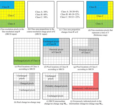
Fig. 2. Production of the intermediate change/no-change map (intermediate Mc/n)

With bi-temporal coarse-resolution class area proportion image cubes P(C) and

P(F), a multiscale land-cover change strategy is applied to downscale these class area

proportion image cubes to produce the intermediate Mc/n by incorporating the input map F. The SRCD method is based on a simplistic view of land-cover change trajectory; this method compares the change in the class area proportion of each class

from the fine-resolution map F to the coarse-resolution image C. If the area proportion of a class in a coarse-resolution pixel appears to be unchanged (e.g., Class

A in Fig. 2), then the number and location of the fine-resolution pixels of that class in

F are unchanged in C. If the area proportion of a class in a coarse-resolution pixel appears to have increased from F to C (e.g., Class B in Fig. 2), then the fine-resolution pixels of that class in F are unchanged, and some fine-resolution pixels in F from class(es) that decreased in class area proportion have transformed into that class in the coarse-resolution image pixel. If the area proportion of a class in a

then the fine-resolution pixels of that class in F include those that may have transformed into fine-resolution pixels of other classes, and no fine-resolution pixels

in F are assumed to have transformed from other classes into that class in the coarse-resolution image pixel. Thus, the fine-resolution pixels of a class in F that decrease in area proportion probably contain the set of changed pixels. As a result, in

F, the fine-resolution pixels with unchanged and increased class area proportions from

F to C (e.g., Class A and Class B in Fig. 2) are probably the unchanged fine-resolution pixels, whereas the fine-resolution pixels with decreased class area proportions from

F to C (e.g., Class C in Fig. 2) are probably the changed fine-resolution pixels in the coarse-resolution pixel. In addition, some unchanged fine-resolution pixels may be

erroneously indicated as being changed pixels in the SRCD intermediate Mc/n (e.g., Class C in Fig. 2 (j)). Thus, SRCD may have overestimated the number of changed

pixels but underestimated the number of unchanged pixels. As a result, the SRCD

intermediate Mc/n contains commission errors of changed pixels and omission errors of unchanged pixels.

3) Iterative Determination Method for Class Area Proportion Change Threshold

In Fig. 2, the omission errors of unchanged pixels are permitted, whereas the

commission errors of unchanged pixels are forbidden. This difference is because the

SRM in SRCD only updates the fine-resolution pixel labels that are changed in the

intermediate Mc/n. If the commission error of unchanged pixels is large, the SRM in SRCD is essentially a traditional SRM that labels all fine-resolution pixels, and the

information in F is merely used. The discrimination of unchanged fine-resolution pixels in the intermediate Mc/n is thus important and is implemented by injecting a threshold t to quantify the amount of unchanged pixels in each coarse-resolution pixel. SRCD employs an iterative class area proportion change thresholding approach,

commission errors of unchanged pixels in the intermediate Mc/n. Through the SRCD iterations, the endmember matrix E is re-estimated, and the accuracy of class area proportion image cube P increases. More potential unchanged fine-resolution pixels should be determined in the intermediate Mc/n. The SRCD is iterated until the completion of a predefined number of iterations.

The iterative SRCD class area proportion change thresholding scheme is

implemented. Let p_ijn be the area proportion difference value of class n in the

coarse-resolution pixel (i,j). It is calculated by subtracting the area proportion value of class n in the pixel (i,j) in the class area proportion image cube P(F) from that in the

class area proportion image cube P(C). Let treal (treal 0) be the real threshold value

for detecting class area proportion change. On the basis of the multiscale land-cover

change strategy, the fine-resolution pixels with unchanged class area proportion

(p_ijn [ t_real,t_real]) or increased class area proportion (p_ijn(t_real,1]) from F to C

are labeled as unchanged in the intermediate Mc/n. Let tini be the initial threshold

value and t be the iterative threshold value. The threshold value t is iteratively decreased from a high value that approximates the higher bound of 1 to a low value

that approximates the lower bound of t_real at an interval of t (t <0) to

gradually detect the increased and unchanged pixels. Initially, t is set to a high value, and fine-resolution pixels with progressively increasing class area proportion from F

to C(p_ijn t) are labeled as unchanged in the intermediate Mc/n. Then, t _{is gradually}

decreased at an interval of t, and more fine-resolution pixels with increased or unchanged class area proportion are labeled as unchanged based on the criterion

ijn t

p

  . When t approximates the t_real value, the p_ijn t criterion ensures that

all the fine-resolution pixels with increased class area proportion (p_ijn(t_real,1]) and

unchanged class area proportion (p_ijn [ t_real,t_real]) are correctly detected and

fine-resolution pixels are gradually reduced.

4) SRM

SRM in SRCD is used to produce the fine-resolution land-cover map Mclass by updating fine-resolution pixels which are changed in the intermediate Mc/n. In SRCD, the spatial-spectral managed algorithm proposed by Ling et. al [18] is modified only

to label changed fine-resolution pixel labels. This SRM is simple implement and has

fast convergence rate. In addition, this SRM has the similar objective function with

the Markov-random-field-based SRM, yet it does not require the endmembers

covariance matrix information as Markov-random-field-based SRM does [15].

The SRM algorithm comprises a spatial term, a spectral term, and a balance

parameter. The spatial term encodes prior knowledge on land-cover spatial patterns

assuming that spatially proximate observations of a given property are more similar

than distant observations. The spectral term measures the spectral difference between

the observed and synthetic pixel spectra. The balance parameter is utilized to balance

the contributions of the spatial and spectral terms.

The objective function (E) of SRM is characterized as

(1 )

spatial spectral

E  E   E (6)

where spatial

E is the spatial term, spectral

E is the spectral term, and  is the balance

parameter.

The SRM spatial term aims to maximize the spatial dependence of neighboring

fine-resolution pixels based on the maximal spatial dependence model, given that the

spatially proximate observations of a given property are more similar than more

distant observations [41]. The spatial term for the k-th(k1, ,s2) fine-resolution pixel in coarse-resolution pixel (i,j), a_{ij k,} , is computed as





_

_{ }



ij k ij k l

l a ij k l

E c a c a c a

d a a  





N

. (7)

,

inside a square window whose center is a_{ij k,} (a_{ij k,} itself is not included in the

window), and a_l is a neighborhood fine-resolution pixel of a_{ij k,} in N(a_{ij k,} ). Here,

the size of the neighborhood N(a_{ij k,} ) was set to 2×s-1 [16, 42]. d a





class labels for fine-resolution pixels a_{ij k,} and a_l. 





,

( _{ij k}) ( )_l

c a c a and 1 otherwise.

The spectral term is utilized to link the observed remotely sensed image to the

fine-resolution labeled map being modeled. The area proportion of class n in pixel (i,j), pijn, is calculated by spatially degrading the fine-resolution label map Mclass according to the scale factor. The SRM spectral term for coarse-resolution pixel (i,j) is expressed as

 

1 1

,

N N

spectral

ij ijn n ij ijn n

n n

E i j p p

 

   

_  _{ }  _

c





Therefore, the objective function (E) of SRM is calculated as





 

2

,

1 1 1 1 1

( ) (1 ) ,

I J s I J

spatial spectral ij k

i j k i j

E  E c a  E i j

    

 





The accuracy of SRM is dependent on the balance parameter that balances the

spatial and spectral terms. When the balance parameter yields a relatively low value

for the spatial term, the land-cover class area proportions barely change, and the prior

land-cover spatial patterns have little influence on Mclass. Conversely, when the balance parameter yields a relatively high value for the spatial term, Mclass may be oversmoothed, and the spectral information provided by the observed remotely sensed

image may be lost [42].

An adaptive balance parameter estimation method for SRM in SRCD is proposed.

The optimal balance parameter is estimated based on the energy balance analysis

proposed by Tolpekin and Stein [42]. If a fine-resolution pixel label, with its true label

,

( _{ij k})

in the spatial term becomes spatial

E

 , and that in the spectral term becomes spectral

E



simultaneously. Therefore, to generate the correct class label on this fine-resolution

pixel, the local contribution on the goal energy from the considered fine-resolution

pixel should be lower for c a( _{ij k,} ) than for c a( _{ij k,} ), and it necessitates the

contribution of the spectral term to compensate for the gain of the spatial term. The

limiting value of  is determined to balance the changes in the spatial and spectral

terms in (10).

spatial spectral

E E

   (10)

The change in the spatial term spatial

E_

 is formulated as





l l l

l a

E_ q  a   c a   c a q 

 



where

,

N( _{ij k}) ( ) 1l

l a  a 



weights of the spatial term. The parameter  depends on the neighborhood system

size and the configuration of class labels ( )c a_l in the neighborhood N(a_{ij k,} ). The

parameter  _{value can be set as a constant [16, 42] or be estimated automatically}

[43]. In this paper, the parameter  _{is set to 0.03 according to [16, 42] for simplicity.}

The change in the spectral term spectral

E_

 before and after the update of the pair of

fine-resolution pixel labels can be formulated as

T 2 2 spectral E s s             _{    }    

e e e e

. (12)

Once spatial

E

 and spectral

E

 are calculated, a range of the balance parameters

that all satisfy (10) can be derived. Solving spatial spectral

E_ E_

   and recalling

/ (1 )

q q

  , the optimal value * is acquired as

* 1 1 _spectral E_   _  

If   *, the model will result in oversmoothing. On the other hand, an extremely low value of  does not fully utilize the spatial information in the model.

The value of spectral

E_

 is related to the class spectral separability, and the average

value Espectral is suggested to be used as a substitute for spectral

E

 when class

separability values for different pairs of classes are different [42].

1 1 1 ( 1) 2 N N spectral a spectral E E N N        

 

 

Equation (13) is then rewritten as

* 1 1 spectral E   _  

. (15)

5) SRCD Energy Minimization

The optimal Mclassis generated by minimizing the SRCD objective function in (6). The SRM problem is characterized by a large solution space. Simulated annealing has

been proposed to solve various global optimization problems, and avoid being trapped

in the local minimum by controlling the acceptance of some inferior solutions which

increase the objective function's value [44]. The acceptance of inferior solutions is

dependent on a parameter κm. κm is iteratively changed according to

1

m m

    _ . (16)

The parameter (0,1) controls the rate of temperature decrease. With the

decrement of κm, the inferior solutions will be accepted with low probability, and

simulated annealing terminates when κm is very small where the global minimum of

the objective function is reached. The initial temperature κm was set to 3, the maximal

iteration number was set to 120, and the parameter  was set to 0.9 [16, 42].

SRCD is iterated until the threshold value reaches a predefined value or a

predefined number of iteration has been completed. Once SRCD converged, Mclass is compared with F to generate the fine-resolution land-cover change/no-change map

SRCD Method

Objective: Estimate fine-resolution change/no-change map Mc/n and from–to

change map Mf-t

Input: Fine-resolution land-cover map F, coarse-resolution image C, scale factor

s between F and C. 1. Initialization:

Set the initial threshold t_ini, step threshold t, the initial iteration number ite=0 and total iteration number itetotal

2. Using F as the initial Mclass

3. Iteratively SRCD do

{

ite=ite+1

Spatially degrade Mclass to class area proportion image cube P(M)(class

area proportion image cube calculated from Mclass) according to scale factor s

Estimate endmember matrix E using C and P(M) based on linear mixture

model

Unmix C based on E to P(C) (class area proportion image cube calculated

from C)

Spatially degrade F to class area proportion image cube P(F) (class area

proportion image cube calculated from F) according to scale factor s Calculate class area proportion difference image P(C)- P(F)

Update threshold t value: t=t_iniite t

Detect the area proportion change of each class in each coarse-resolution pixel

Generate the intermediate Mc/n based on threshold t

Use SRM to update labels of fine-resolution pixels in Mclass which are

changed in the intermediate Mc/n

}

until ite= itetotal

4. Producing the final Mc/n and Mf-t

Per-pixel comparison of F and Mclass

Result: Mc/n and Mf-t

E. Accuracy Metric

The pixel-based quality metrics were used to assess the accuracy of Mc/n and Mf-t by comparing the result change maps with the reference data. The accuracies of the

accuracies of the different land-cover from–to changes in Mf-t were also assessed. The accuracies of the changed and unchanged pixels in the intermediate Mc/n produced by the multiscale land-cover change strategy from P(C) and P(F) or final Mc/n produced by per-pixel comparison between Mclass and F were measured using the omission error, commission error, and F1-score. The F1-score is the harmonic mean of precision,

which represents the measure of exactness or quality, and recall, which represents the

measure of completeness or quantity [46]. The per-class accuracies of different

land-cover from–to changes in Mf-t were assessed using the producer’s and user’s accuracies.

III. E

A

R

Experiments using synthetic multispectral image, real MODIS multispectral

remotely sensed image and real Landsat-8 multispectral image were conducted in

order to assess the proposed SRCD method. The fine-resolution map post-dated the

coarse-resolution image in the synthetic image experiment, and pre-dated the

coarse-resolution image in the MODIS and Landsat-8 image experiments. SRCD is

not compared with other methods, because there is, to our knowledge, no other

method focusing on the extraction of fine-resolution land-cover change information

using different spatial resolution images without prior endmember information.

A. Synthetic Image Experiment

1) Data Preparation

A synthetic multispectral image was used in this experiment. The test data were

obtained based on NLCD in 2001 and 2006, respectively. NLCD is a land-cover

classification scheme that has been applied consistently at a spatial resolution of 30 m

across the U.S.A.. NLCD is based primarily on the unsupervised classification of

Landsat satellite data. NLCD 2001 and 2006 are geo-registered to the Albers Equal

Area projection grid [47]. There are 16 land-cover classes in NLCD. Introducing too

many classes would affect the spectral unmixing accuracy for linear mixture model

reclassified into 4 classes, namely, Water-Wetlands (WW), Developed-Barren (DB),

Shrubland-Herbaceous (SH), and Planted/Cultivated (PC).

The reference fine-resolution map was generated from NLCD 2001, and the

input fine-resolution map was generated from NLCD 2006. Both maps contain 800 ×

800 pixels located in Charlotte (Fig. 3). The changed fine-resolution pixels account

for 7.8% of all pixels in the study area. The input coarse-resolution multispectral

image was simulated from the fine-resolution reference map. A fine-resolution

multispectral image was produced first. The number of bands was set to 6 to

accommodate for a dimensionality constraint in spectral unmixing. The 4 endmember

signature digital number (DN) values were set to [750, 400, 225, 20, 80, 130]T, [310,

70, 107, 390, 360, 330] T, [160, 295, 455, 605, 720, 960] T, and [440, 520, 750, 890,

980, 520] T. T is the transposition operator. The covariance matrices for all the classes

were set to A·I, where A=500 is a constant and I is 6 by 6 identity matrix [42]. The fine-resolution multispectral image was first produced according to the reference map

and class endmembers. The spectral response of each class was normally distributed

in each waveband. The fine-resolution multispectral image was then spatially

degraded to the coarse-resolution multispectral image with the scale factor s=10. The reference fine-resolution land-cover change/no-change map and from–to change map

were produced by a per-pixel comparison of the NLCD 2001 and 2006 land-cover

Fig. 3. SRCD input and reference images of synthetic image experiment. The zoomed area contains 100 × 100 fine-resolution pixels.

The initial SRCD parameters were set. The initial class area proportion change

threshold value, t_ini, can be set between 0 and 1. A high t_ini value would extend the

SRCD convergence time, whereas a low tini value would eliminate small-sized

unchanged land-cover patches in the intermediate change/no-change map. Thus, the

initial class area proportion change threshold value was set to t_ini 0.5. A low t

value would extend the SRCD convergence time, whereas a high t _{value would} reduce the number of unchanged land-cover patches in the intermediate and final

change/no-change maps. Thus, the step class area proportion change threshold value

was set to   t 0.05. The number of total iterations was set to itetotal= 20. SRCD is

terminated with a class area proportion change threshold value of

0.5

ini total

tt ite   t . The SRCD results are shown in Fig. 4.

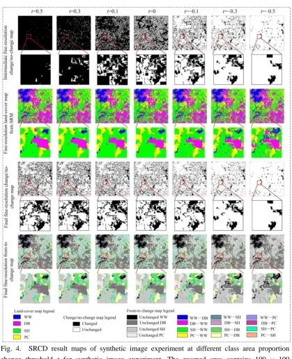
Fig. 4. SRCD result maps of synthetic image experiment at different class area proportion

change threshold t for synthetic image experiment. The zoomed area contains 100 × 100

fine-resolution pixels.

Fig. 4 summarizes the SRCD results, highlighting the intermediate

fine-resolution change/no-change maps used for SRM, the fine-resolution land-cover

maps generated by SRM, and the final output fine-resolution change/no-change maps

and from–to change maps at different class area proportion change threshold t values. More fine-resolution pixels were indicated as having changed labels in the

intermediate change/no-change map than in the final output change/no-change maps

to the fine-resolution pixels indicated as changed in the intermediate

change/no-change map, which indicated parts of the changed pixels in the

intermediate change/no-change map as unchanged pixels in the final

change/no-change map.

The performance of SRCD varied with the class area proportion change

threshold t. When the threshold is t0.3, most fine-resolution pixels were indicated as having changed in the intermediate change/no-change map. The changed

fine-resolution pixel labels were determined by SRM. Many rounded patches were

evident in the subset images because SRM adopted the land-cover maximum spatial

dependence model, which could have oversmoothed the land-cover patches. With the

decrease in threshold t, more fine-resolution pixels were detected as unchanged in the intermediate change/no-change map, and more land-cover patches in the input

fine-resolution map, which were identified as unchanged, were preserved in the

land-cover map produced by SRM. More unchanged fine-resolution pixels were also

observed in the final fine-resolution change/no-change and from–to change maps.

When the threshold is t  0.3, most fine-resolution pixel labels in the input fine-resolution map with unchanged class area proportion were preserved in the

land-cover map, and the final change/no-change and from–to change maps were

approximate to the reference maps.

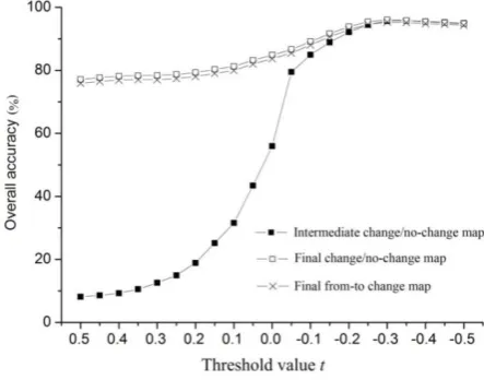
Fig. 5. Overall accuracies of intermediate change/no-change maps, final change/no-change maps, and final from–to change maps for synthetic image.

well as the final from–to change maps, are shown in Fig. 5. The overall accuracies of

all the maps increased gradually with a decrease in threshold t when t is higher than −0.3 and decreased with a decrease in threshold t when t is lower than −0.3. The final

change/no-change maps exhibited a higher overall accuracy than the intermediate

change/no-change maps for each threshold t value. This result is due to difference in the data sources used for generating these maps: the intermediate change/no-change

map was produced using the class area proportion information at the coarse-resolution

scale, whereas the final change/no-change map was produced by comparing

land-cover maps at the fine-resolution scale. The highest overall accuracies of the

final change/no-change map and the from–to change maps were 96.00% and 95.28%,

respectively, when t 0.3.

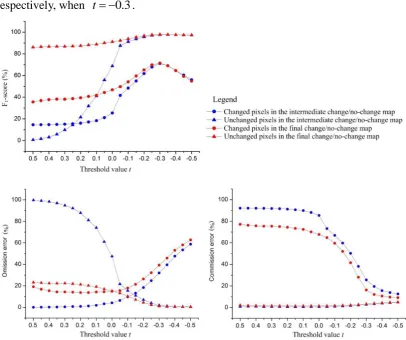
Fig. 6. The F1-scores, omission errors, and commission errors of unchanged and changed

fine-resolution pixels in the intermediate and final fine-resolution change/no-change maps for the synthetic image experiment.

The accuracies of the intermediate and final change/no-change maps were

in Fig. 6. The F1-score for the changed pixels in the intermediate and final

change/no-change maps increased gradually with a decrease in threshold t when t is higher than −0.3, and decreased when the threshold t is lower than −0.3 because many

changed pixels were erroneously identified as unchanged pixels. The intermediate and

final change/no-change maps have the highest F1-score (higher than 71%) for changed

pixels when the threshold t 0.3. The F1-scores for unchanged pixels in the intermediate and final change/no-change maps increased gradually with a decrease in

threshold t when t is higher than −0.3 and remained almost unchanged when the threshold t is lower than −0.3. The highest F1-score for unchanged pixels was higher than that for changed pixels in the intermediate and final change/no-change maps.

This is because most pixels were unchanged in the study area, and the majority of

pixels were identified as unchanged by SRCD when the threshold t 0.3. The final change/no-change maps produced by comparing land-cover maps at the

fine-resolution scale have higher F1-scores for changed and unchanged pixels than the

intermediate change/no-change maps produced using the class area proportion

information at the coarse-resolution scale at most threshold t values.

The omission errors of unchanged pixels decreased with a decrease in threshold t. This result is because most unchanged fine-resolution pixels were initially indicated

as having changed; however, with a decrease in threshold t, the detected unchanged fine-resolution pixels increased, and more unchanged fine-resolution pixels were

correctly detected. By contrast, the omission errors of changed pixels increased with a

decrease in threshold t because almost all fine-resolution pixels were initially detected as having changed. With a decrease in threshold t, the detected changed fine-resolution pixels decreased, and more actually changed pixels were erroneously

identified as unchanged.

The commission errors of changed pixels decreased with a decrease in threshold

t. This result is because almost all the fine-resolution pixels were initially detected as having changed; however, with a decrease in threshold t, the detected changed fine-resolution pixels decreased, and many of the initially erroneously detected

errors of unchanged pixels were low and remained almost unchanged with a decrease

in threshold t. When threshold t is lower than −0.3, the commission errors of the unchanged pixels increased, whereas the commission errors of the changed pixels

decreased with a decrease in threshold t. Therefore, more changed pixels were erroneously detected as unchanged, and less unchanged pixels were erroneously

detected as changed.

Fig. 7. The producer's accuracy and user's accuracy of different land-cover from–to changes for synthetic image experiment.

The producer’s accuracy and user’s accuracy of different land-cover from–to

changes for the synthetic image experiment are shown in Fig. 7. The producer’s

accuracies of WW—WW, DB—DB, SH—SH, and PC—PC increased with a decrease

in threshold t, whereas the producer’s accuracies of the other land-cover changes decreased with a decrease in threshold t. The number of correctly detected unchanged classes increased, whereas the number of correctly detected changed classes

decreased. The producer’s accuracies of DB—PC and WW—SH were 0% because

only 13 fine-resolution pixels had a DB—PC change and 62 fine-resolution pixels had

a WW—SH change in the 2001–2006 reference from–to change map. These changed

patches were smaller than a coarse-resolution pixel, which contained s2=100 fine-resolution pixels. The producer’s accuracies of unchanged classes have a

dominant effect on the global accuracy in the from–to change map because more than

accuracies of unchanged classes decreased, whereas those of the changed classes

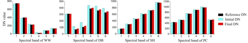
increased with a decrease in threshold t. Fig. 8 shows the reference endmember signatures, extracted initial endmember signatures at t0.5, and extracted final endmember signatures at t 0.3 . A good match between the reference and estimated endmember signatures was observed at t 0.3.

Fig. 8. Reference endmember signatures (reference DN), estimated endmember signatures at 0.5

t  (initial DN) and at t  0.3 (final DN) for the synthetic image experiment.

B. MODIS Image Experiment

1) Data Preparation

MODIS multispectral images were adopted to assess SRCD based on real

remotely sensed images. The study area is located near Sorriso (12º33'21"S and

55º42'31"W) in Mato Grosso State, Brazil. This area is in the Brazilian Amazon Basin,

and is mainly covered by tropical forests but which has undergone a deforestation in

recent years. The experiment data include a Landsat-5 TM image with a spatial

resolution of 30 m acquired on August 13, 2000, a Landsat-7 ETM+ image with a

spatial resolution of 30 m acquired on July 18, 2005, and a single eight-day surface

reflectance MODIS product (MOD09A1) with a spatial resolution of 463 m taken in

July 2005. The TM image was geo-registered to the ETM+ image. The TM image

acquired in 2000 was digitized to the input fine-resolution land-cover map with forest

and nonforest in it, and the ETM+ image acquired in 2005 was digitized to the

reference map. The MODIS image comprising 7 spectral bands (620 nm - 2055 nm)

was used as the SRCD input coarse-resolution image. The MODIS image was

re-projected into the Universal Transverse Mercator coordinate system and then

resampled to a spatial resolution of 450 m using the nearest neighbor algorithm. A

ETM+ images were adopted (Fig. 9). The scale factor s is set to 15. The changed fine-resolution pixels account for 22.8% of all pixels in the study area.

SRCD was implemented for the scenarios in which the fine-resolution map

pre-dated the coarse-resolution image. The reference fine-resolution land-cover

change/no-change map and from–to change map were produced by a per-pixel

comparison of the 2000 and 2005 land-cover maps. The SRCD parameters were set as

in the synthetic image experiment: t_ini 0.5,   t 0.05, and itetotal=20.

Fig. 9. SRCD input and reference images of MODIS image experiment. The zoomed area contains 300 × 300 fine-resolution pixels.

Fig. 10. Experimental results of MODIS image experiment

The input images, reference maps, and result maps are shown in Fig. 9 and Fig.

10. Deforestation occurred in the region during the periods represented. Some of the

deforestations exhibited a fishbone pattern because of the expansion of the nonforest

patch (such as the left zoomed area), whereas some of the deforestations were in

clear-cut areas (such as the right zoomed area). More pixels were detected as

unchanged pixels with a decrease in threshold t. As a result, the changed pixels marked in black decreased, whereas the unchanged pixels marked in white increased

in the intermediate and final change/no-change maps. The changed land-cover

trajectories marked in blue and red decreased, whereas the unchanged land-cover

trajectories marked in gray increased in the from–to change maps with a decrease in

threshold t. In the reference from–to change map in Fig. 9, forest–nonforest change trajectory patches marked in red were more than nonforest–forest change trajectory

trajectory in the study area. Most of the spatial patterns of the changed land-cover

trajectories were correctly mapped onto the from–to change map when t 0.3. The forest–nonforest patches were mapped with rounded shape, and some of the spatial

details were lost. This result is attributed to the use of the land-cover maximal spatial

dependence model by SRM in producing the changed land-cover patches; this model

could oversmooth class boundaries.

Fig. 11. The F1-scores for changed and unchanged pixels in the intermediate and final

fine-resolution change/no-change maps for MODIS image experiment.

Fig. 11 shows the F1-scores for changed and unchanged pixels in the

intermediate and final fine-resolution change/no-change maps. For changed pixels,

the intermediate change/no-change maps obtained F1-scores lower than 50% when

0

t  and obtained F1-scores higher than 60% when t0. For unchanged pixels, the F1-scores obtained by the intermediate change/no-change maps were lower than 50%

when t 0 and higher than 80% when t0. The final change/no-change maps have F1-scores higher than 60% for changed pixels and higher than 90% for

unchanged pixels. The highest F1-score of the final change/no-change map is

Fig. 12. The producer's accuracy and user's accuracy of different land-cover from–to changes for MODIS experiment.

Fig. 12 shows the producer’s and user’s accuracies of different land-cover

from–to changes at different threshold t values. The producer’s accuracies of nonforest–nonforest and forest–forest changes increased, whereas the producer’s

accuracies of forest–nonforest and nonforest–forest changes decreased because more

fine-resolution pixels were detected as unchanged with a decrease in threshold t. The producer’s accuracies of nonforest–nonforest and forest–forest changes were higher

than those for forest–nonforest and nonforest–forest changes. This result is because

the unchanged pixel labels were determined by the input fine-resolution land-cover

map, whereas the changed pixel labels were determined by SRM. The producer’s

accuracy of forest–nonforest change was higher than that for nonforest–forest change.

The main reason is that the forest–nonforest patches were usually larger than the

coarse-resolution pixel; thus, SRM with the maximum land-cover spatial dependence

model was suitable for mapping these patches [24]. By contrast, nonforest–forest

patches were usually found along patch boundaries with linear shapes wherein the

SRM may have oversmoothed the patches. The pixel number of the nonforest–forest

change accounts for 2.0% of all the pixels, and the pixel number of the

forest–nonforest change accounts for 20.7% of all the pixels in the 2000–2005

reference fine-resolution from–to change map. Thus, the forest–nonfores change

detection accuracy has a more dominant effect on the overall change detection

whereas those of changed classes increased with a decrease in threshold t. This result is because the number of pixels of changed classes marked in blue and red decreased,

whereas the number of pixels of unchanged classes marked in gray increased with a

decrease in threshold t. The overall accuracy of the form–to change map increased from 83.27% when t0.5 to 87.15% when t  0.3 and then decreased to 85.98% when t  0.5.

C. Landsat-8 OLI Image Experiment

1) Data Preparation

A Landsat multispectral images was adopted as the coarse-resolution image in

this experiment. The study area is located in Wuhan (30º21'70"N and 114º15'19"E),

China. A Landsat-8OLI image acquired on June 13, 2013 was selected as the relative

coarse-resolution image. The Landsat-8 OLI image has 9 multispectral bands. The

first 7 bands of OLI image with a spatial resolution of 30 m were selected as the

coarse-resolution image for SRCD input. The 8th band (panchromatic band) of OLI

image was not used because it has a spatial resolution of 15 m, and the 9th band (cirrus

band) of OLI image was not used because it is not suitable for detecting land-covers.

Two Google Earth optical images with fine spatial resolution, which were acquired on

August 14, 2010 and on June 13, 2013 were selected. The Google Earth optical

images were geo-registered to the ETM+ image. The 2010 Google Earth image was

digitized to the SRCD input previous fine-resolution land-cover map, and the 2013

Google Earth image was digitized to the reference map. There are 4 land-cover

classes in the fine-resolution maps, which are water, grass, impervious surface and

bareland. A subset of 40 × 40 pixels Landsat-8 OLI image was used as the SRCD

input coarse-resolution image. The previous and reference land-cover maps contains

200 × 200 pixels (Fig. 13). The scale factor s is set to 5. The changed fine-resolution pixels account for 12.5% of all pixels in the study area. The reference fine-resolution

land-cover change/no-change map and from–to change map were produced by a

were set as in the synthetic and MODIS image experiments: tini 0.5,   t 0.05,

and itetotal=20.

Fig. 13. SRCD input and reference images of Landsat-8 OLI image experiment.

2) Results

Fig. 14. Experimental results of Landsat-8 OLI image experiment.

in subsets A to F in the reference from–to change map. The grass–bareland changes in

subsets C, D, and E were mainly caused by the expansion of the previously bareland.

Other land-cover changes were unremarkable, such as in subset G. In Fig. 13, more

pixels were identified as unchanged pixels with a decrease in threshold t. In the final change/no-change maps, the changed pixels marked in black decreased, whereas the

unchanged pixels marked in white increased with a decrease in threshold t. In the final from–to change maps, the land-cover changes marked in color decreased with a

decrease in threshold t. The erroneously detected from–to changes (bareland–grass and water–grass) in the bottom-left corner of the image appeared when t 0.3 and disappeared when t 0.3. This result may be attributed to the fact that the bareland and water patches in the bottom-left corner were small in the reference map and were

detected as changed and oversmoothed by SRM when t 0.3. The grass–bareland changes in subsets A to E were detected in the from–to change maps when t 0.5. The shapes of the changed patches were smoothed because of the spatial smoothing

effect of SRM. As a result, the grass–bareland changes in subsets A and B had

rounded shapes; being smaller than the coarse-resolution pixel, grass–bareland

changes in subset F were eliminated in the from–to change map because of the

oversmoothing effect of SRM. The grass–bareland changes in subset C were detected

as having a linear shape when t  0.5 and were similar to those in the reference from–to change map in Fig. 13. Some of the changed patches that were smaller than

Fig. 15. The F1-scores for changed and unchanged pixels in the intermediate and final

fine-resolution change/no-change maps for Landsat image experiment.

Fig. 15 shows the F1-scores for changed and unchanged pixels in the

intermediate and final fine-resolution change/no-change maps. The F1-scores for

changed pixels in the intermediate and final change/no-change maps increased

gradually with a decrease in threshold t when t  0.3, and decreased when the 0.3

t  . The F1-score for unchanged pixels in the intermediate and final change/no-change maps gradually increased with a decrease in threshold t when

0.3

t  and remained almost unchanged when t 0.3. The highest F1-score for changed pixels was 56.39% in the intermediate change/no-change map when

0.3

t  and 61.37% in the final change/no-change map when t 0.3.