remote sensing
Article
Assessing a Temporal Change Strategy for Sub-Pixel
Land Cover Change Mapping from Multi-Scale
Remote Sensing Imagery
Feng Ling1,2,*, Giles M. Foody2, Xiaodong Li1, Yihang Zhang1and Yun Du1
1 Key Laboratory of Monitoring and Estimate for Environment and Disaster of Hubei Province, Institute of Geodesy and Geophysics, Chinese Academy of Sciences, Wuhan 430077, China; [email protected] (X.L.); [email protected] (Y.Z.); [email protected] (Y.D.) 2 School of Geography, University of Nottingham, University Park, Nottingham NG7 2RD, UK;
* Correspondence: [email protected]; Tel.: +86-27-6888-1901
Academic Editors: Parth Sarathi Roy and Prasad S. Thenkabail
Received: 31 May 2016; Accepted: 1 August 2016; Published: 6 August 2016
Abstract:Remotely sensed imagery is an attractive source of information for mapping and monitoring land cover. Fine spatial resolution imagery is typically acquired infrequently, but fine temporal resolution systems commonly provide coarse spatial resolution imagery. Sub-pixel land cover change mapping is a method that aims to use the advantages of these multiple spatial and temporal resolution sensing systems. This method produces fine spatial and temporal resolution land cover maps, by updating fine spatial resolution land cover maps using coarse spatial resolution remote sensing imagery. A critical issue for sub-pixel land cover change mapping is downscaling coarse spatial resolution fraction maps estimated by soft classification to a fine spatial resolution land cover map. The relationship between a historic fine spatial resolution map and a contemporary fine spatial resolution map to be estimated at a more recent date plays an important role in the downscaling procedure. A change strategy based on the assumption that the change for each land cover class in a coarse spatial resolution pixel is unidirectional was shown to be a promising means to describe this relationship. This paper aims to assess this change strategy by analyzing the factors that affect the accuracy of the change strategy, using six subsets of the National Land Cover Database (NLCD) of USA. The results show that the spatial resolution of coarse pixels, the time interval of the previous fine resolution land cover map and the current coarse spatial resolution images, and the thematic resolution of the used land cover class scheme have considerable influence on the accuracy of the change strategy. The accuracy of the change strategy decreases with the coarsening of spatial resolution, an increase of time interval, and an increase of thematic resolution. The results also indicate that, when the historic land cover map has a 30 m resolution, like the NLCD, the average accuracy of the change strategy is still as high as 92% when the coarse spatial resolution data used had a resolution of ~1000 m, confirming the effectiveness of the change strategy used in sub-pixel land cover change mapping for use with popular remote sensing systems.
Keywords: sub-pixel mapping; spatial scale; temporal change pattern; land cover change; change strategy
1. Introduction
Land cover change has been considered as one of the most important drivers of the global environmental change [1–3]. Timely and accurate monitoring of these changes is crucial for many scientific research fields such as ecology, agriculture and hydrology. Presently, it has been widely recognized that remote sensing is an attractive source of information on land cover change [4–6].
Remote sensing provides the ability to acquire images of the Earth’s surface at a range of scales, notably in the spatial and temporal domains. Systems such as the Moderate Resolution Imaging Spectroradiometer (MODIS) provide data at a fine temporal resolution but coarse spatial resolution, while others such as Landsat sensors provide imagery with a relatively fine spatial but coarse temporal resolution. By using a variety of remote sensing systems it should be possible to use multi-scale data to monitor land cover at fine spatial and temporal scales [7]. Generally, once a baseline fine spatial resolution land cover map has been generated from fine spatial resolution images, it then should be possible to update it in a timely manner through the use of coarse spatial resolution images, if the limitation of their coarse spatial resolution can be reduced.
When coarse spatial resolution remote sensing images are used to generate land cover data, a critical issue is the mixed pixel problem [8–11]. Because the sensor’s instantaneous field-of-view (IFOV) includes more than one land cover class on the ground, the spectral characteristics of mixed pixels are not representative of any single land cover class. In this situation, a mixed pixel cannot be appropriately represented by conventional hard classification technologies that consider a pixel to be a unit comprised of a single land cover class. Soft classification can overcome this problem to some extent, by indicating the class composition (e.g., the areal percentage cover of land cover classes in each coarse resolution pixel) [12–14]. The comparison of a time series of soft classifications allows a richer representation of land cover change, as it allows fractional land cover conversions and modifications to be characterized. However, a fuller appreciation of land cover change needs not only information on the quantity of land cover class coverage in the area represented by pixels but also on the spatial configuration of landscapes in the region mapped [15,16]. In practice, when a coarse spatial resolution image is used to detect land cover change by comparing with a previous fine spatial resolution image, a popular method is applying soft classification on the coarse spatial resolution image and spatially degrading the fine spatial resolution image to generate two coarse spatial resolution area proportion images. By comparing the bi-temporal area proportion images, the change in the class proportions of each coarse spatial resolution pixel is detected. However, with this approach, only the coarse spatial resolution area change instead of the fine spatial resolution location change was detected, and the spatial information included in the fine spatial resolution image is not used. Thus, in order to better understand the nature and impacts of land cover change, it is necessary to determine the spatial configuration of land cover classes at the fine spatial resolution.
In the remote sensing community, the method used to determine the spatial land cover configuration at a finer spatial resolution than that at which the source imagery were acquired is often called as sub-pixel mapping [17]. Sub-pixel mapping can be considered to be a post-processing stage of soft classification, in which the fraction images produced by soft classification are used as input to estimate a hard land cover map with fine spatial resolution [18]. A variety of sub-pixel mapping algorithms have been proposed, such as Hopfield neural networks [19–21], pixel-swapping algorithm [22], Markov random field [23], spatial attraction algorithms [24–28], vectorial boundary based algorithms [29,30], computational intelligence algorithms [31–33], and spatial regularization algorithm [34–37]. Sub-pixel mapping has been successfully used in many applications, such as the mapping urban trees [38], lakes [39], burned area [40] as well as in the refinement of ground control point location [41] and in the calculation of landscape pattern indices [42].
Most sub-pixel mapping algorithms have been applied to single date remotely sensed imagery. Thus, to update a historic fine resolution land cover map with contemporary coarse fraction map, an intuitive method is to directly generate a fine resolution land cover map from the coarse fraction map using sub-pixel mapping algorithms and undertaking a post-classification comparison to indicate the change. Although this approach seems sensible, it fails to take account of the initial land cover pattern in the historic dataset.
Remote Sens.2016,8, 642 3 of 23
modeling [43,44]. In land use change models, such as the CLUE-S model [45], land use scenarios are simulated by using socio-economical and biophysical driving factors. The simulated land use scenarios typically have a very coarse spatial resolution and need to be downscaled to a fine resolution. For a typical downscaling algorithm, the relationships between driving factors (such as elevation, distance to river, etc.) and land use patterns are first estimated. The relationships are then used when simulating the competition between land use types for a specific location at the fine spatial resolution. Special land use type or location specific decision rules can also be specified by the user according to the historic fine resolution land use map. Finally, the historic fine resolution map is updated with these relationship and the simulated land use map at a more recent date obtained.
The advantages of the scenario downscaling algorithms in land use change modeling lies in the relationships between driving factors and land cover patterns, and the decision rules. However, for sub-pixel mapping algorithms used with remote sensing imagery, this relationship is often unavailable and the land cover change rules are often difficult to specify. In order to overcome this problem, Ling et al. [46] proposed a sub-pixel land cover change mapping model, which aims to generate a new fine spatial resolution land cover map, by updating a historic fine resolution land cover map using contemporary coarse resolution fraction images directly. This approach not only exploits the general concept of sub-pixel mapping, but also relates the target fine spatial resolution land cover map that we aim to estimate with available historic fine resolution land cover map, through a land cover change strategy.
A sub-pixel land cover change mapping model generally consists of two different sub-models [46,47]. The first is the spatial sub-model, which is the spatial prior model used to describe the spatial pattern of land cover classes in traditional sub-pixel mapping algorithms. The second is the temporal sub-model, which is used to describe the relationship between the historic and current fine resolution land cover maps. In order to construct a suitable temporal sub-model in the sub-pixel land cover change mapping model, an effective land cover change strategy is required. At present, the change strategy proposed by Ling et al. [46] is widely used [47–54]. This change strategy is referred to as the unidirectional change strategy in this paper; because it is generally based on an assumption that the landscape keeps relative stability, and supposes that only unidirectional change exists within a small area. With this unidirectional change strategy, various temporal sub-models can be constructed and used in sub-pixel land cover change mapping [46–54].
Both the spatial and temporal sub-models play important roles in the sub-pixel land cover change mapping model. Compared with the spatial sub-model that has been widely studied in sub-pixel mapping, however, the temporal sub-model has attracted relatively little attention in the literatures. Although previous studies have illustrated the effectiveness of sub-pixel land cover change mapping, the individual impact of the temporal sub-model on the result has not been reported. Regarding the significant role of the temporal sub-model in sub-pixel land cover change mapping, and the unidirectional change strategy is again the basis of most exiting temporal sub-models, this paper aims to assess the unidirectional change strategy thoroughly. By analyzing the fundamental principle behind the unidirectional change strategy, the main factors that influence the accuracy of the change strategy were explored, in order to provide guidance for its practical application.
2. The Unidirectional Change Strategy
2.1. Sub-Pixel Mapping
land cover class. The resulting fine spatial resolution land cover map thus containspSˆMq ˆ pSˆNq
pixels, whose labels are defined to a unique land cover class.
The objective of sub-pixel mapping is to make the fine spatial resolution land cover map honor a pre-defined spatial pattern model, according to the number of fine spatial resolution pixels within each coarse spatial resolution pixel provided by the input fraction images. Therefore, the final fine spatial resolution land cover map should be produced according to an area constraints and a spatial model. The area constraints is used to restrict the estimated fine spatial resolution land cover map to the input coarse spatial resolution fraction images, and the spatial model is used to incorporate prior information about the land cover distribution. From the viewpoint of optimization, the sub-pixel mapping problem can be expressed as the following minimization problem:
MinEpxq “Eareapxq `λEspatialpxq (1)
whereEareapxqis the area constraints term andEspatialpxqis the spatial model term.λis the parameter used to balance the area constraints term and the spatial model term.
Various methods have been proposed to construct both terms, leading to different sub-pixel mapping models. For the area constraints term, in some models, the number of sub-pixels for each land cover class in each mixed pixel is restricted so that it corresponds with input area fractions [22,55], while other models relax the constraints caused by fraction images in order to eliminate the fraction errors caused by soft classification [19,21,34]. For the spatial model term, the spatial dependence model that aims to make the fine spatial resolution land cover map have the maximal spatial dependence is widely used [19,22,34,56]. The spatial model can also be constructed through the incorporation of information provided by additional dataset [57,58], or learned from the training image [59–61]. A comprehensive review of these models is beyond the scope of this paper, and more information can be found in relative literatures.
2.2. Sub-Pixel Land Cover Change Mapping
Sub-pixel land cover change mapping is an extension of sub-pixel mapping. Suppose that there is another historic fine spatial resolution land cover map of the region available, besides the current coarse spatial resolution fraction images generated via a soft classification analysis. The aim of sub-pixel land cover change mapping is to determine the change information of each pixel in the historic fine resolution map with the aid of current coarse resolution fraction images. If the current coarse resolution fraction images can be downscaled to a fine resolution map, the land cover change information can be simply obtained by directly comparing both fine resolution land cover maps. In other words, sub-pixel land cover change mapping is also a sub-pixel mapping problem. A special feature is that, when producing the current fine spatial resolution map, not only the current coarse spatial resolution fraction images, but also the land cover information included in the historic fine spatial resolution map are considered.
Generally, in order to use the information provided by the historic fine resolution land cover map, a temporal model needs to be defined to represent the relationship between the historic fine resolution land cover map and the current coarse resolution fraction images. Based on the sub-pixel mapping model as shown in Equation (1), the sub-pixel land cover change mapping problem can be extended as the following minimization problem:
MinEpxq “Eareapxq `λEspatialpxq `γEtemporalpxq (2)
whereEtemporalpxqis the temporal model term andγis the balance parameter.
Remote Sens.2016,8, 642 5 of 23
resolution pixel labels are not allowed to change as the analysis proceeds, and remaining fine spatial resolution pixel labels are estimated by traditional sub-pixel mapping algorithms. An alternative approach first generated transfer probabilities between all land cover classes in each coarse spatial resolution pixel, which was then used to produce the temporal model term used in the optimization model [47].
In general, the relationship between the historic fine spatial resolution land cover map and the current spatial coarse resolution fraction images can be described by a land cover change strategy, because the spatial land cover configuration at the current time is affected by the historic configuration. The unidirectional change strategy [46], which is widely used at present, is presented as follow.
2.3. The Unidirectional Change Strategy
GivenSis the scale factor, which is the ratio between the coarse and fine resolution pixels, there are S2fine resolution pixels within the area represented by a coarse resolution pixel. LetLbe a current coarse resolution pixel andHbe its corresponding historicS2fine resolution pixels. For each coarse resolution pixel, there is a set of fraction values representing the area percentage for each land cover class contained in the pixel. The current land cover fractionsfpLqcan be estimated by soft classification, and the historic land cover fractionsfpHqcan also be extracted through spatially degradingHusing a mean filter with anSˆSfine resolution window.
By comparing the fractions in fpHqand fpLq, three categories of fractional change can be defined: class(es) of unchanged fraction, class(es) that decrease in fractional coverage and class(es) that increase in fractional coverage of the geographical area represented by a coarse resolution pixel. The unidirectional change strategy then defines different change rules for each of these three land cover change categories. For the class of unchanged fraction, no change is permitted. Thus, fine resolution pixels belonging to this class in H should be absolutely preserved. For a class that decreases in fractional coverage, fine resolution pixels belonging to this class inHcan be changed to other classes, and fine resolution pixels belonging to other classes inHshould not be changed to this class. Finally, for the class that increases in fractional coverage, fine resolution pixels belonging to this class are all preserved, and some fine resolution pixels belonging to other classes are changed to this class.
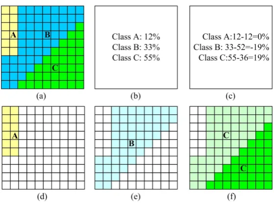
A simple example is used to illustrate the change strategy in Figure1. In this example, the scale factor is 10 and hence a coarse resolution pixel contains 10ˆ10 fine resolution pixels. There are three land cover classes: A, B and C. By considering those fine resolution pixels as a coarse resolution pixel, the fractions of class A, B and C are 12%, 52% and 36%, respectively. Accordingly, there are 12 fine resolution pixels labeled as class A, 52 fine resolution pixels labeled as class B and 36 fine resolution pixels labeled as class C (Figure1a). With the passage of time, land cover may change from that depicted in the historic fine resolution pixels. Suppose that the current fractions of class A, B and C become 12%, 33% and 55% (Figure1b). The fraction changes of each class are computed using the fractions in the historic and current coarse resolution pixels (Figure1c). However, the result in Figure1c can show only the fractional coverage and not the geographical distribution of the classes. To study land cover change in detail, the geographical location of the fractions and their change in time needed to be determined by sub-pixel land cover change mapping.
Remote Sens. 2016, 8, 642; doi:10.3390/rs8080642 6 of 23
Figure 1. An example of land cover change and allocation of fine resolution pixel labels according to the change strategy: (a) historic 10 × 10 fine resolution pixels in a coarse resolution pixel; (b) corresponding current coarse resolution mixed pixel, where class fractions of each class are denoted; (c) fraction change of each class; (d) fine resolution pixel locations of class A marked in yellow color in the current fine resolution map; (e) potential fine resolution pixel locations of class B marked in light blue color in the current fine resolution map; and (f) fine resolution pixel locations of class C marked in dark green color and potential fine resolution pixel locations for the rest of class C marked in light green color in the current fine resolution map.
2.4. The Scale Issue
According to the unidirectional change strategy, for any land cover class, fine resolution changed-in and changed-out pixels do not appear within the area of a coarse resolution pixel at the same time. The scale factor between the coarse and fine resolution pixels is expected to strongly affect the performance of the change strategy. In extreme cases, if the scale factor equals to 1, which means the historic fine resolution map and current coarse resolution map have the same spatial resolution, all fine resolution pixels obey the change strategy. Conversely, if the scale factor is extremely high, a coarse resolution pixel may cover thousands of kilometers and millions of fine resolution pixels, increasing the possibility of change within the pixel area not being unidirectional. Therefore, in which situation the change strategy is obeyed becomes a critical issue for its practical application.
3. Dataset and Methods
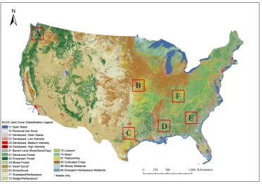
The National Land Cover Database (NLCD) was used to assess the change strategy. The NLCD contains raster-based land cover maps with a 30 m × 30 m spatial resolution over all 50 states and Puerto Rico across the conterminous United States of America [62,63]. NLCD 2001, NLCD 2006 and NLCD 2011 are based primarily on decision-tree classifications of Landsat satellite data acquired in circa 2001, 2006 and 2011, respectively, and include 16 land cover classes modified from the Anderson land-use and land-cover classification system (Table 1). The study areas selected are six subsets of NLCD maps, each 240 km × 240 km (8000 pixels × 8000 pixels) in size (Figure 2). The land cover change percentage, which is calculated through a per-pixel comparison of land cover types, is presented in Table 2. The six areas each experienced land cover change but of differing magnitude and spatial distribution. Areas A, D and E experienced a high land cover change during 2001–2006 and 2001–2011, whereas area F experienced the least land cover change. In Figure 3, the changed land cover pixels are relatively centralized in area A and B. In areas D and E, the changed land cover pixels are not represented as aggregated patches, but are spatially distributed across the entire map. By contrast, large parts of the map do not contain changed pixels in areas C and F.
Figure 1.An example of land cover change and allocation of fine resolution pixel labels according to the change strategy: (a) historic 10ˆ10 fine resolution pixels in a coarse resolution pixel; (b) corresponding current coarse resolution mixed pixel, where class fractions of each class are denoted; (c) fraction change of each class; (d) fine resolution pixel locations of class A marked in yellow color in the current fine resolution map; (e) potential fine resolution pixel locations of class B marked in light blue color in the current fine resolution map; and (f) fine resolution pixel locations of class C marked in dark green color and potential fine resolution pixel locations for the rest of class C marked in light green color in the current fine resolution map.
2.4. The Scale Issue
According to the unidirectional change strategy, for any land cover class, fine resolution changed-in and changed-out pixels do not appear within the area of a coarse resolution pixel at the same time. The scale factor between the coarse and fine resolution pixels is expected to strongly affect the performance of the change strategy. In extreme cases, if the scale factor equals to 1, which means the historic fine resolution map and current coarse resolution map have the same spatial resolution, all fine resolution pixels obey the change strategy. Conversely, if the scale factor is extremely high, a coarse resolution pixel may cover thousands of kilometers and millions of fine resolution pixels, increasing the possibility of change within the pixel area not being unidirectional. Therefore, in which situation the change strategy is obeyed becomes a critical issue for its practical application.
3. Dataset and Methods
Remote Sens.2016,8, 642 7 of 23
Remote Sens. 2016, 8, 642; doi:10.3390/rs8080642 7 of 23
Figure 2. Locations of the six study areas as shown in the National Land Cover Database (NLCD) 2011 land cover map.
[image:7.595.113.486.88.349.2]Figure 3. Land cover maps (240 km × 240 km, 8000 pixels × 8000 pixels with the 30 m spatial resolution) and corresponding land cover change map (black indicates the changed pixels) for the six study areas.
The NLCD is available with 16 classes. As land cover change studies often focus on a relatively low number of classes, the original 16 classes were aggregated to form two new data sets with eight and four classes, respectively (Table 1), to assess the impact of the thematic resolution on the accuracy of change mapping. Table 2 shows the land cover change ratio, which represents the
Figure 2.Locations of the six study areas as shown in the National Land Cover Database (NLCD) 2011 land cover map.
Remote Sens. 2016, 8, 642; doi:10.3390/rs8080642 7 of 23
Figure 2. Locations of the six study areas as shown in the National Land Cover Database (NLCD) 2011 land cover map.
[image:7.595.111.488.398.700.2]Figure 3. Land cover maps (240 km × 240 km, 8000 pixels × 8000 pixels with the 30 m spatial resolution) and corresponding land cover change map (black indicates the changed pixels) for the six study areas.
The NLCD is available with 16 classes. As land cover change studies often focus on a relatively low number of classes, the original 16 classes were aggregated to form two new data sets with eight and four classes, respectively (Table 1), to assess the impact of the thematic resolution on the accuracy of change mapping. Table 2 shows the land cover change ratio, which represents the
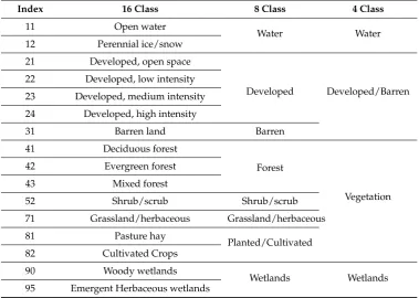
Table 1.The land cover class grouping strategy.
Index 16 Class 8 Class 4 Class
11 Open water
Water Water
12 Perennial ice/snow
21 Developed, open space
Developed Developed/Barren 22 Developed, low intensity
23 Developed, medium intensity 24 Developed, high intensity
31 Barren land Barren
41 Deciduous forest
Forest
Vegetation
42 Evergreen forest
43 Mixed forest
52 Shrub/scrub Shrub/scrub
71 Grassland/herbaceous Grassland/herbaceous
81 Pasture hay
Planted/Cultivated
82 Cultivated Crops
90 Woody wetlands
Wetlands Wetlands
95 Emergent Herbaceous wetlands
Table 2.Land cover changed area percentages for different areas during 2001–2006 and 2001–2011.
2001–2006 2001–2011
16 Class 8 Class 4 Class 16 Class 8 Class 4 Class
A 5.99% 5.94% 0.93% 11.33% 10.78% 4.12%
B 1.10% 1.08% 0.99% 2.22% 1.44% 1.26%
C 1.32% 1.28% 0.55% 4.83% 4.26% 2.12%
D 7.25% 6.98% 0.91% 14.16% 13.13% 1.42%
E 7.05% 6.92% 1.62% 13.96% 13.05% 2.74%
F 0.59% 0.58% 0.31% 1.92% 1.28% 0.74%
The NLCD is available with 16 classes. As land cover change studies often focus on a relatively low number of classes, the original 16 classes were aggregated to form two new data sets with eight and four classes, respectively (Table1), to assess the impact of the thematic resolution on the accuracy of change mapping. Table2shows the land cover change ratio, which represents the percentage of pixels with changed classes (a high value means the study area has a highly dynamic landscape during the period). The changed area percentages for the 16-class scheme in different areas are only slightly higher than those for the eight-class scheme. The changed area percentages for the four-class scheme decreased compared with those of 16-class and eight-class schemes in the different study areas, because the inter-class changes for 16-class and eight-class schemes become intra-class changes for the four-class scheme. The highest changed area percentage was 14.16% for the 16-class scheme in area D during 2001–2011, and the lowest changed area percentage was 0.31% for the four-class scheme in area F during 2001–2006.
[image:8.595.152.445.417.520.2]Remote Sens.2016,8, 642 9 of 23
current fine spatial resolution land cover maps directly. Simulating coarse spatial resolution fraction images can avoid extra fraction errors caused by the soft classification and the spatial registration error between fine and coarse spatial resolution images. Moreover, the original fine spatial resolution land cover maps can be used as the reference to assess the result.
In each case, the NLCD 2001 subsets were used as the previous fine spatial resolution land cover maps, and NLCD 2006 or NLCD 2011 subsets were used to simulate what is described here as the current coarse resolution fraction images, respectively. When the coarse fraction images were simulated, different thematic resolution (4, 8 and 16 classes) and different scale factors including 4, 8, 10, 16, 33, 50, 100, 200, 500 and 1000, which correspond to the spatial resolution of 120 m, 240 m, 300 m, 480 m, 990 m, 1.5 km, 3 km, 6 km, 15 km, and 30 km, respectively, were applied. Therefore, in this experiment, the total number of simulated cases is 360: 6 (study area)ˆ2 (NLCD 2006 or NLCD 2011)ˆ3 (thematic resolution)ˆ10 (scale factor). In each case, the coarse resolution fraction images can be produced by spatial degradation processing, by dividing the number of fine resolution pixels of each class by the total number of fine resolution pixels in a coarse resolution pixel, according to used dataset and parameters.
The change strategy accuracy (Acs) value that represents the percentage of fine resolution pixels obeying the change strategy was used to assess the accuracy of the change strategy in each scenario. Let fpLqcbe the fraction of class c in the current coarse resolution pixel and fpHqcbe that in the corresponding historic coarse resolution pixel that is degraded from fine resolution pixels. The fraction change of class c in current and historic coarse resolution pixels, called∆fc, is determined as∆fc “ fpLqc´fpHqc. Assuming the label of a historic fine resolution pixeliis classc, whether the fine resolution pixeliobeys the change strategy is determined according to the class label of its corresponding current fine resolution pixeljas the following:
(1) If ∆fc = 0, the fraction of classcis unchanged. According to the change strategy about the unchanged-fraction class, fine resolution pixels belonging to this class in historic and current maps should be the same. Then, if the current fine resolution pixeljis also classc, the corresponding fine resolution pixeliin the historic map obeys the change strategy. If, however, pixeljbelongs to another class than that depicted for pixeli, the change strategy is disobeyed.
(2) If∆fc> 0, the fraction of classcincreases. According to the change strategy, all fine resolution pixels belonging to this class in the historic map need to be preserved in the current map. Then, if the current fine resolution pixeljis classc, the fine resolution pixeliobeys the change strategy. Otherwise, pixelidisobeys the change strategy.
(3) If∆fc< 0, the fraction of classcdecreases. In this case, if the current fine resolution pixel jis also classc, the fine resolution pixeli obeys the change strategy. In addition, fine resolution pixels belonging to classes that decreased in fraction may change to the increased-fraction class according to the change strategy. Then, if the current fine resolution pixeljbelongs to the class that has increased fraction, the fine resolution pixelialso obeys the change strategy.
Figure5e obey the change strategy and the pixels shown as black in Figure5e do not obey the change strategy. In summary, there are seven pixels in the fine spatial resolution map that do not obey the change strategy, as shown in FigureRemote Sens. 2016, 8, 642; doi:10.3390/rs8080642 5f. 10 of 23
Figure 4. The flowchart used to judge whether a fine resolution pixel within a coarse resolution pixel obeys the change strategy or not.
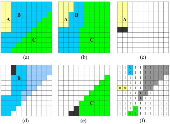
[image:10.595.159.438.492.696.2]Figure 5. An example of
A
cs calculation: (a) Historic fine resolution pixels within a coarse resolution pixel. The scale factor is 10; (b) Corresponding current fine resolution pixels; (c–e) Fine resolution pixels of class A, B and C, as shown in (a), respectively. Pixels marked in color obey the change strategy, and pixels marked in black do not obey the change strategy; (f) The final indicator map, where 1 means that the pixel obeys the change strategy, and 0 means that the pixel does not obey the change strategy. Pixels marked in color and grey are changed pixels.Figure 4.The flowchart used to judge whether a fine resolution pixel within a coarse resolution pixel obeys the change strategy or not.
Remote Sens. 2016, 8, 642; doi:10.3390/rs8080642 10 of 23
Figure 4. The flowchart used to judge whether a fine resolution pixel within a coarse resolution pixel obeys the change strategy or not.
Figure 5. An example of
A
cs calculation: (a) Historic fine resolution pixels within a coarse resolution pixel. The scale factor is 10; (b) Corresponding current fine resolution pixels; (c–e) Fine resolution pixels of class A, B and C, as shown in (a), respectively. Pixels marked in color obey the change strategy, and pixels marked in black do not obey the change strategy; (f) The final indicator map, where 1 means that the pixel obeys the change strategy, and 0 means that the pixel does not obey the change strategy. Pixels marked in color and grey are changed pixels.Remote Sens.2016,8, 642 11 of 23
According to the aforementioned steps,Acsis calculated according to the number of fine resolution pixels that obey the change strategy. Moreover, in order to better represent the ability of the change strategy to describe the land cover change scenario, and to avoid the bias caused by different changed area percentages, only fine resolution pixels whose land cover labels in the historic and current maps are different, are included to calculate the value ofAcsas:
Acs“ nc
´nd
nc (3)
wherendis the number of pixels that disobey the change strategy, andncis the number of pixels that changed class label. Take Figure5as an example,ndequals to 7 andncequals to 29, including the pixels as shown in grey in Figure5f. Thus, the value ofAcsis 0.759% or 75.9%. TheAcsvalue represents the percentage of fine spatial resolution pixels obeying the change strategy in all changed fine spatial resolution pixels, and a higherAcsvalue indicates that the change strategy represents the temporal land cover change pattern better.
4. Results
The change mapping approach was applied to the NLCD data for each time period and each study area. The resultingAcsvalues are shown in Table3. Moreover, Figure6shows theAcsvalues for six study areas with land cover maps of NLCD during 2001 and 2006, and Figure7shows those during 2001 and 2011. Generally,Acsvalues vary with the scale factor, the thematic resolution and the changed area percentage.
Remote Sens. 2016, 8, 642; doi:10.3390/rs8080642 11 of 23
According to the aforementioned steps,
A
cs is calculated according to the number of fine resolution pixels that obey the change strategy. Moreover, in order to better represent the ability of the change strategy to describe the land cover change scenario, and to avoid the bias caused by different changed area percentages, only fine resolution pixels whose land cover labels in the historic and current maps are different, are included to calculate the value ofA
cs as:c d cs
c
n
n
A
n
−
=
(3)where
n
d is the number of pixels that disobey the change strategy, andn
c is the number of pixels that changed class label. Take Figure 5 as an example,n
d equals to 7 andn
c equals to 29, including the pixels as shown in grey in Figure 5f. Thus, the value ofA
cs is 0.759 or 75.9%. TheA
cs value represents the percentage of fine spatial resolution pixels obeying the change strategy in all changed fine spatial resolution pixels, and a higherA
cs value indicates that the change strategy represents the temporal land cover change pattern better.4. Results
[image:11.595.85.516.386.644.2]The change mapping approach was applied to the NLCD data for each time period and each study area. The resulting
A
cs values are shown in Table 3. Moreover, Figure 6 shows theA
cs values for six study areas with land cover maps of NLCD during 2001 and 2006, and Figure 7 shows those during 2001 and 2011. Generally,A
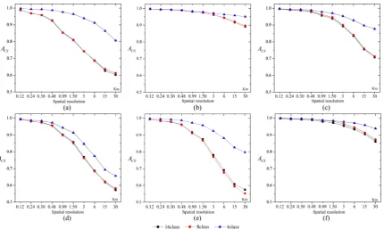
cs values vary with the scale factor, the thematic resolution and the changed area percentage.Figure 6. The
A
cs values during 2001–2006 with different land cover class schemes. (a–f) Represent the results of the study areas A to F, respectively.Table 3.Acsvalues for six study areas with different spatial resolution of coarse pixels, land cover class schemes and time spans.
Area TimeSpan Class Scheme
Spatial Resolution of Coarse Pixels 120 m
(S= 4)
240 m (S= 8)
300 m (S= 10)
480 m (S= 16)
990 m (S= 33)
1.5 km (S= 50)
3 km (S= 100)
6 km (S= 200)
15 km (S= 500)
30 km (S= 1000)
A
2001–2006
16 class 0.987 0.967 0.957 0.925 0.855 0.809 0.742 0.686 0.627 0.602
8 class 0.987 0.967 0.956 0.923 0.853 0.808 0.742 0.688 0.637 0.613
4 class 0.998 0.994 0.993 0.987 0.975 0.963 0.938 0.912 0.864 0.806
2001–2011
16 class 0.961 0.928 0.913 0.876 0.804 0.761 0.696 0.641 0.585 0.555
8 class 0.962 0.929 0.914 0.876 0.804 0.762 0.696 0.643 0.586 0.555
4 class 0.954 0.922 0.909 0.879 0.819 0.776 0.698 0.629 0.564 0.513
B
2001–2006
16 class 0.997 0.994 0.992 0.988 0.980 0.975 0.960 0.943 0.916 0.892
8 class 0.997 0.993 0.992 0.988 0.979 0.973 0.960 0.943 0.921 0.897
4 class 0.997 0.994 0.993 0.990 0.983 0.979 0.970 0.962 0.957 0.950
2001–2011
16 class 0.991 0.981 0.977 0.965 0.941 0.920 0.873 0.822 0.770 0.731
8 class 0.997 0.993 0.992 0.988 0.979 0.974 0.960 0.944 0.921 0.897
4 class 0.996 0.992 0.989 0.984 0.971 0.962 0.946 0.929 0.914 0.900
C
2001–2006
16 class 0.996 0.989 0.986 0.978 0.955 0.938 0.893 0.835 0.755 0.707
8 class 0.996 0.991 0.989 0.981 0.961 0.945 0.899 0.840 0.760 0.712
4 class 0.998 0.994 0.993 0.989 0.977 0.970 0.952 0.927 0.897 0.877
2001–2011
16 class 0.979 0.958 0.948 0.924 0.871 0.833 0.761 0.699 0.637 0.596
8 class 0.984 0.967 0.959 0.938 0.887 0.849 0.778 0.717 0.654 0.617
4 class 0.991 0.977 0.972 0.956 0.920 0.895 0.845 0.798 0.739 0.692
D
2001–2006
16 class 0.992 0.980 0.974 0.956 0.903 0.857 0.767 0.688 0.618 0.572
8 class 0.992 0.980 0.974 0.954 0.898 0.851 0.761 0.685 0.621 0.582
4 class 0.994 0.986 0.983 0.972 0.943 0.914 0.846 0.773 0.693 0.656
2001–2011
16 class 0.980 0.957 0.946 0.915 0.837 0.782 0.693 0.629 0.587 0.559
8 class 0.984 0.963 0.953 0.921 0.843 0.788 0.701 0.637 0.585 0.573
4 class 0.991 0.981 0.977 0.963 0.926 0.897 0.828 0.757 0.685 0.627
E
2001–2006
16 class 0.993 0.984 0.978 0.962 0.917 0.875 0.781 0.692 0.608 0.575
8 class 0.993 0.983 0.978 0.961 0.912 0.867 0.769 0.678 0.594 0.552
4 class 0.997 0.994 0.992 0.987 0.973 0.958 0.925 0.881 0.827 0.798
2001–2011
16 class 0.982 0.962 0.952 0.924 0.858 0.807 0.721 0.661 0.613 0.588
8 class 0.987 0.969 0.961 0.934 0.869 0.820 0.736 0.683 0.644 0.625
4 class 0.996 0.991 0.988 0.981 0.965 0.952 0.924 0.892 0.852 0.841
F
2001–2006
16 class 0.997 0.993 0.991 0.988 0.979 0.972 0.954 0.934 0.905 0.860
8 class 0.998 0.996 0.995 0.993 0.986 0.981 0.965 0.945 0.914 0.872
4 class 0.999 0.997 0.996 0.993 0.987 0.984 0.978 0.970 0.958 0.939
2001–2011
16 class 0.971 0.944 0.935 0.912 0.872 0.846 0.796 0.740 0.667 0.626
8 class 0.994 0.988 0.985 0.978 0.961 0.943 0.905 0.863 0.812 0.791
4 class 0.997 0.993 0.991 0.986 0.976 0.964 0.943 0.920 0.903 0.892
Remote Sens.2016,8, 642 13 of 23
[image:13.595.86.512.86.349.2]Remote Sens. 2016, 8, 642; doi:10.3390/rs8080642 14 of 23
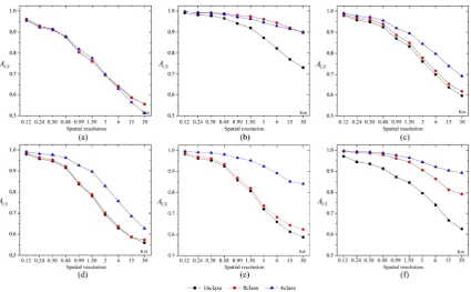
Figure 7. The
A
cs values during 2001–2011 with different land cover class schemes. (a–f) Representthe results of the study areas A to F, respectively.
4.1. The Spatial Resolution
As shown in Figures 6 and 7,
A
cs values decrease with the increase of the spatial resolution ofcoarse pixels. That is, the coarsening of the spatial resolution of coarse pixels results in more pixels not obeying the change strategy. When the spatial resolution of coarse pixels is 120 m, that is, the
scale factor is 4, the average
A
cs value is 0.989, meaning that 98.9% changed pixels obey the changestrategy. When the spatial resolution of coarse pixels is 990 m (
S
=
33
), the averageA
cs value isstill as high as 0.92. The
A
cs value at the 990 m spatial resolution of coarse pixels is different indifferent study areas, the highest one is 0.987, and the lowest one is 0.804. With the further increase
of the spatial resolution of coarse pixels, however, the
A
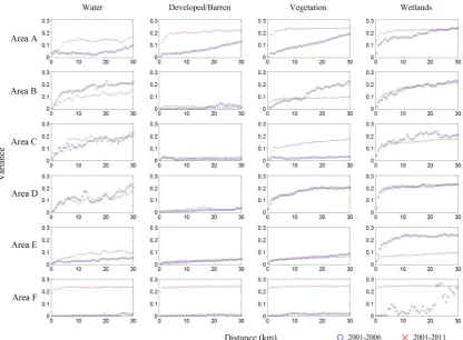
cs values decrease rapidly.The spatial pattern of land cover is important for sub-pixel mapping [64]. For sub-pixel land cover change mapping, the spatial pattern of temporal land cover change also affects the accuracy of the change strategy. According to the fundamental principle of the change strategy, for each land cover class within a coarse resolution pixel, only unidirectional changes exist and changed-out and changed-in pixels do not exist simultaneously. Figure 8 shows the scatter plot of variance values versus the distance of changed-out and changed-in pixels for each land cover class during 2001–2006 and 2001–2011 in the four-class scheme result and Figure 9 shows those in the eight-class scheme. A larger variance value means that more bidirectional land cover changes exist.
In general, the variance values are small with a small distance for all these scenarios. For example, most of the first variance values calculated with the distance of 0.6 km are much less than 0.1 in all scenarios. This means that, for a random changed fine spatial resolution pixel, the probability that another changed pixel with a distance of 0.6 km to it has the same change direction is larger than 90%. From another point of view, in a coarse pixel with the spatial resolution of 0.6 km, more than 90% of changed pixels have the same change direction. The variance value becomes larger with the increment of distance. This tread means that more fine spatial resolution pixels have different change directions when their spatial distance becomes larger. In other words, with the increment of the spatial resolution of coarse pixels, more bidirectional changes exist in a coarse
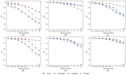
Figure 7.TheAcsvalues during 2001–2011 with different land cover class schemes. (a–f) Represent the results of the study areas A to F, respectively.
4.1. The Spatial Resolution
As shown in Figures6and7,Acsvalues decrease with the increase of the spatial resolution of coarse pixels. That is, the coarsening of the spatial resolution of coarse pixels results in more pixels not obeying the change strategy. When the spatial resolution of coarse pixels is 120 m, that is, the scale factor is 4, the averageAcsvalue is 0.989, meaning that 98.9% changed pixels obey the change strategy. When the spatial resolution of coarse pixels is 990 m (S“33), the average value is still as high as 0.92. TheAcsvalue at the 990 m spatial resolution of coarse pixels is different in different study areas, the highest one is 0.987, and the lowest one is 0.804. With the further increase of the spatial resolution of coarse pixels, however, theAcsvalues decrease rapidly.
The spatial pattern of land cover is important for sub-pixel mapping [64]. For sub-pixel land cover change mapping, the spatial pattern of temporal land cover change also affects the accuracy of the change strategy. According to the fundamental principle of the change strategy, for each land cover class within a coarse resolution pixel, only unidirectional changes exist and changed-out and changed-in pixels do not exist simultaneously. Figure8shows the scatter plot of variance values versus the distance of changed-out and changed-in pixels for each land cover class during 2001–2006 and 2001–2011 in the four-class scheme result and Figure9shows those in the eight-class scheme. A larger variance value means that more bidirectional land cover changes exist.
Remote Sens.resolution pixel. This explains the result that the 2016,8, 642
A
cs values decrease with the coarsening of the 14 of 23 spatial resolution of coarse pixels. [image:14.595.91.508.87.393.2]Figure 8. The variance values for the six study areas during 2001–2006 and 2001–2011 with different land cover classes in the four-class scheme.
Figure 9. The variance values for the six study areas during 2001–2006 and 2001–2011 with different land cover classes in the eight-class scheme.
Figure 8.The variance values for the six study areas during 2001–2006 and 2001–2011 with different land cover classes in the four-class scheme.
Remote Sens. 2016, 8, 642; doi:10.3390/rs8080642 15 of 23
resolution pixel. This explains the result that the
A
cs values decrease with the coarsening of thespatial resolution of coarse pixels.
[image:14.595.90.508.457.723.2]Figure 8. The variance values for the six study areas during 2001–2006 and 2001–2011 with different land cover classes in the four-class scheme.
Figure 9. The variance values for the six study areas during 2001–2006 and 2001–2011 with different land cover classes in the eight-class scheme.
Remote Sens.2016,8, 642 15 of 23
From Figures6and7, it also noticed that the decline rates of theAcsvalues are much different in different scenarios. This is mainly caused by the pattern of variance values. As shown in Figures8and9, with the increase of the distance, the variance values show various change patterns. In some scenarios, such as the area B in 2001–2006 in the four-class scheme, the variance values decline at a near-linear trend for the vegetation and wetlands classes. As a result, theAcsvalue has a near-linear decline rate. By contrast, in the area D in 2001–2006 in the four-class scheme, the variance values for the vegetation and wetlands classes first decline rapidly within about 2 km, and then decline slowly. As a result, theAcsvalue has a much higher decline rate at the beginning.
4.2. The Time Interval
The time interval between the previous fine spatial resolution land cover map and the current coarse spatial resolution images affects the accuracy of the change strategy. As shown in Figures6and7, theAcsvalues are different at the 2001–2006 and 2001–2011 periods. The changed area percentages in all six areas during 2001–2006 and 2001–2011 are shown in Table2. For a certain area, the changed area percentage during 2001–2011 was always higher than that during 2001–2006, as the area would have more possibility to change if it experiences a longer period of time (Table2). As a result, almost allAcs values for 2001–2011 (Figure7) were lower than the correspondingAcsvalues for 2001–2006 (Figure6).
From Figures8and9, it is noticed that the time interval had an important role on the variance values. In most cases, the variance values during 2001–2011 were larger than those during 2001–2006. During 2001–2011, the number of fine spatial resolution pixels that changed their class labels was much larger than that during 2001–2006. This made the land cover change pattern more complex and the inter-change of land cover classes more popular, leading to a larger variance value. For different land cover classes, the variance values were also different. For example, in the area A in the four-class scheme, the variance value of the developed/barren class almost equals to zero during 2001–2006, but increased rapidly during 2001–2011. As a result, theAcsvalue during 2001–2011 is much lower than that during 2001–2006 in the area A.
4.3. The Thematic Resolution
As shown in Figure6, for the land cover change during 2001–2006, theAcsvalues decrease with the increment of the thematic resolution. The simplest four-class land cover scheme was always associated with the highest Acs values. TheAcs values observed for analyses with the eight-class and 16-class schemes are basically the same, and both much lower than that of the four-class scheme. For the land cover change during 2001–2011 (Figure7), a similar trend was noticed where the scheme with lowest number of land cover classes often obtained highAcsvalues. In some areas, however, the difference between the eight-class and 16-class schemes becomes distinguishable.
In general, the changed area percentage is larger when the thematic resolution increases, as shown in Table2. It is noteworthy that the four-class scheme was generated from the eight-class scheme, which was again generated from the 16-class scheme in this experiment. For a class changed to another class in the eight-class scheme, the change still existed in the four-class scheme if these two classes belonged to different classes in the four-class scheme. While these two classes belonged to the same class in the four-class scheme, the changed area became the same class and the change did not exist in the four-class scheme. When the thematic resolution was 4, the changed area percentages for all study areas were less than those of the eight-class and 16-class schemes, and the correspondingAcsvalues are mostly higher than those of the eight-class and 16-class schemes.
Remote Sens.2016,8, 642 16 of 23
It is also noticed that theAcsvalues of the four-class scheme are not always higher than those of the eight-class and 16-class schemes. For example, in the area B during the 2001–2011, theAcsvalues of the four-class scheme are lower than those of the eight-class scheme when the spatial resolution of coarse pixels ranges from 1 km to 15 km. This is mainly caused by two reasons. First, the changed area percentage was 1.44% for the eight-class scheme and 1.26% for the four-class scheme. Using the four-class scheme did not much reduce the change area. Second, combining several classes in the eight-class scheme to one class in the four-class scheme may change the used rule of the change strategy. For example, if one class with increased area and another class with decreased area in the eight-class scheme were combined to one class in the four-class scheme, the change strategy becomes ineffective for at least one class in the eight-class scheme, leading to a decreasedAcsvalue.
4.4. Per-Class Analysis
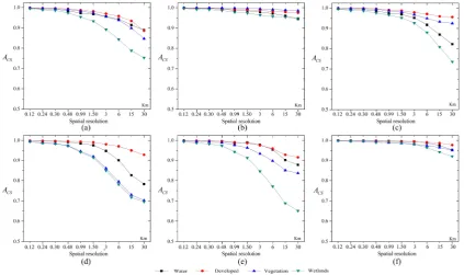
Figures10and11show theAcsvalues obtained for different land cover classes at the four-class scheme, and Table4shows the land cover class transfer matrices in all these areas. Overall, for all land cover classes, the trends of theAcsvalues at the category level are similar with those at the map level discussed above; that is, theAcsvalues decrease with the increase of the scale factor and the increase of the change area.
As shown in Table 2, for all six areas during the 2001–2006 period and most areas during the 2001–2011 period, the changed area percentages of the eight-class and 16-class schemes were very close. This indicated that land cover that changed in the 16-class scheme also changed in the
eight-class scheme. In this situation, the
A
cs values were almost the same for the eight-class and16-class schemes. During 2001–2011, however, the changed area percentages of the eight-class
scheme were different with those of the 16-class scheme in the areas B and F, making the
A
csvalues different.
It is also noticed that the
A
cs values of the four-class scheme are not always higher than thoseof the eight-class and 16-class schemes. For example, in the area B during the 2001–2011, the
A
csvalues of the four-class scheme are lower than those of the eight-class scheme when the spatial resolution of coarse pixels ranges from 1 km to 15 km. This is mainly caused by two reasons. First, the changed area percentage was 1.44% for the eight-class scheme and 1.26% for the four-class scheme. Using the four-class scheme did not much reduce the change area. Second, combining several classes in the eight-class scheme to one class in the four-class scheme may change the used rule of the change strategy. For example, if one class with increased area and another class with decreased area in the eight-class scheme were combined to one class in the four-class scheme, the change strategy becomes ineffective for at least one class in the eight-class scheme, leading to a
decreased
A
cs value.4.4. Per-Class Analysis
Figures 10 and 11 show the
A
cs values obtained for different land cover classes at the four-classscheme, and Table 4 shows the land cover class transfer matrices in all these areas. Overall, for all
land cover classes, the trends of the
A
cs values at the category level are similar with those at themap level discussed above; that is, the
A
cs values decrease with the increase of the scale factor andthe increase of the change area.
Figure 10. The
A
cs values during 2001–2006 for different land cover classes with the four-class [image:16.595.86.510.335.586.2]scheme. (a–f) Represent the results of the study areas A to F, respectively.
Figure 10.TheAcsvalues during 2001–2006 for different land cover classes with the four-class scheme. (a–f) Represent the results of the study areas A to F, respectively.
Remote Sens.2016,8, 642 17 of 23
the ratio of pixels, this abrupt land cover change percentage greatly affected the performance of the change strategy.
Remote Sens. 2016, 8, 642; doi:10.3390/rs8080642 18 of 23
The
A
cs values obtained differed between land cover classes. In most cases, theA
cs values ofthe vegetation and wetlands classes were lower than those of the water and developed/barren classes. One reason for this difference was that the change areas for the vegetation and wetlands classes were larger than those of the water and developed/barren classes (Table 4). Another reason was the stability of land cover classes. In general, water and developed/barren areas were more stable temporally than the vegetation and wetland classes and the change strategy is then more
effective in the water and developed/barren areas. In Figure 11, however, it is apparent that the
A
csvalue decreased in 2001–2011 in area B for the developed/barren class. This is because the number of changed pixels from developed/barren to vegetation rapidly increased in this area from 1758 during
the period 2001–2006 to 41,219 during the period 2001–2011. Because the
A
cs value is a relativevalue that reflects the ratio of pixels, this abrupt land cover change percentage greatly affected the performance of the change strategy.
Figure 11. The
A
cs values during 2001–2011 for different land cover classes with the four-class [image:17.595.82.513.126.383.2]scheme. (a–f) Represent the results of the study areas A to F, respectively.
Table 4.Transfer matrixes for six study areas with the four-class scheme during 2001–2006 and 2001–2011.
2006
Land Cover Water Db Veg Wet Land Cover Water Db Veg Wet
2001
A
Water 3,116,366 19,357 5684 1972
B
Water 791,233 3035 3376 1586
DB 3583 6,994,948 357,820 2611 DB 1766 5,583,533 1758 551
Veg 2195 111,536 51,560,188 49,568 Veg 106,367 131,085 56,076,531 359,721
Wet 2794 11,649 29,473 1,730,256 Wet 15,115 2442 4117 917,784
C
Water 1,098,440 1988 12,326 3043
D
Water 836,413 2735 39,937 4810
DB 2847 5,268,490 8899 290 DB 301 3,612,785 9169 84
Veg 17,128 251,552 54,120,307 32,403 Veg 23,396 87,385 51,442,482 167,987
Wet 5577 7094 7991 3,161,625 Wet 6373 6780 235,585 7,523,778
E
Water 1,176,054 3577 5167 1700
F
Water 891,964 15,936 4019 910
DB 15,803 6,991,968 160,834 1564 DB 1601 4,744,077 3166 269
Veg 36,129 566,439 49,514,204 105,917 Veg 8944 160,284 57,966,901 2199
Wet 9544 8435 1,185,92 5,284,073 Wet 215 1035 2990 195,490
2011
2001
A
Water 3,103,034 29,721 6086 4538
B
Water 789,631 3743 3466 2390
DB 35,254 6,957,042 357,365 9301 DB 3187 5,541,891 41,219 1311
Veg 60,571 535,507 50,392,410 734,999 Veg 110,823 244,845 55,949,346 368,690
Wet 35,572 67,682 761,702 909,216 Wet 16,406 3324 5918 913,810
C
Water 1,092,348 3428 15,598 4423
D
Water 818,683 4333 54,076 6803
DB 3187 5,226,750 50,176 413 DB 571 3,607,785 13,782 201
Veg 41,648 569,663 53,647,536 162,543 Veg 37,792 258,647 51,176,048 248,763
Wet 7673 16,427 483,952 2,674,235 Wet 8707 12,276 263,869 7,487,664
E
Water 1,170,098 6654 6792 2954
F
Water 888,202 15,517 8030 1032
DB 17,851 6,948,926 198,717 4675 DB 2930 4,712,826 33,251 282
Veg 45,980 1,064,314 48,794,496 317,899 Veg 10,992 393,906 57,728,264 5205
Wet 9065 13,020 65,380 5,333,179 Wet 240 1256 3227 194,840
Remote Sens.2016,8, 642 19 of 23
5. Discussion
Sub-pixel land cover change mapping is a relatively new technology in the field of multi-temporal land cover change analysis. This technology expands existing land cover change analysis methods from the pixel to the sub-pixel scale. By using sub-pixel land cover change mapping, a historic fine resolution land cover map can be updated with information from current coarse resolution images. Because coarse resolution remotely sensed imagery often have a high temporal resolution, this new technology enables high spatial and temporal resolution land cover change analysis. Sub-pixel land cover change mapping can be considered as a special sub-pixel mapping method. A key feature of this method is that an existing historic fine spatial resolution land cover map should be incorporated in the sub-pixel mapping model. This historic fine spatial resolution land cover map provides valuable information about the spatial distribution of the various land cover classes in mixed coarse resolution pixels in coarse imagery acquired at a later date.
To use the information provided by the historic fine resolution land cover map, a sub-pixel land cover change mapping model often includes a spatial sub-model and a temporal sub-model. The spatial prior model used in existing sub-pixel mapping algorithms, such as the maximal spatial dependence, can be used directly as the spatial sub-model. The temporal sub-model can provide the information of land cover pattern included in the historic map to the current map, and ensure the consistency of multi-temporal fine resolution land cover maps. Therefore, although the change strategy itself cannot absolutely determine the class labels of current fine resolution pixels, it still plays a very important role in sub-pixel land cover change mapping.
The results of the experiments reported above show that the performance of the change strategy is substantially affected by the spatial resolution of coarse pixels, the time interval of the previous fine spatial resolution land cover map and the current coarse spatial resolution images, and the thematic resolution of the used land cover class scheme. According to the experiments, firstly, the accuracy of the change strategy decreases with the coarsening of the spatial resolution of coarse pixels. If the fine resolution map have a resolution of ~30 m, like the NLCD, the average accuracy of the change strategy is about 92% when the coarse spatial resolution data used had a resolution of ~1000 m. Secondly, the accuracy of the change strategy decreases with the increment of the time interval between the fine spatial resolution land cover map and the coarse spatial resolution images, with which there are often more changed areas. Therefore, in the area with rapid land cover changes, more recently high spatial resolution land cover maps should be collected as the baseline for land cover change mapping, in order to improve the accuracy of the change strategy. Thirdly, the accuracy of the change strategy decreases with the increment of the number of land cover classes. In practice, the soft classification, which is used to estimate fraction maps, often uses a simple land cover class scheme comprising a low number of classes. For example, in the linear mixture model, the number of classes should be less than the bands of data used. This situation is consistent with the usage of the change strategy.
6. Conclusions
Fine spatial and temporal resolution land cover datasets are valuable information for many scientific research fields. Sub-pixel land cover change mapping is a recently proposed method that aims to update a fine spatial resolution land cover dataset using coarse spatial resolution remote sensing images with a high temporal resolution. In sub-pixel land cover change mapping models, the temporal model plays a crucial role to the result. The unidirectional change strategy is a popular method to describe the relationship between the historic fine resolution map and current coarse resolution fraction images, and to construct the temporal model in sub-pixel land cover change mapping. In this paper, the factors that affect the accuracy of the unidirectional change strategy were analyzed, in order to provide guidance for the practical application of the approach to sub-pixel land cover change mapping from multi-scale remote sensing images.
The experiment was performed by using six subsets of the NLCD maps, each 240 kmˆ240 km in size. The results of experiments indicate the accuracy of the change strategy is mainly affected by the spatial resolution of coarse pixels, the time interval of the previous fine spatial resolution land cover map and the current coarse spatial resolution images, and the thematic resolution of the used land cover class scheme. With the coarsening of the spatial resolution, the percentage of the changed pixels that obeys the change strategy decreases because the spatial dependence of changed-out and changed-in pixels decreases with the increase of distance between changed pixels. An increase of the time interval or the thematic resolution often increases the changed area and the variance values of land cover change, leading to a decrease of the accuracy of the change strategy, In the future, more experiments should be performed in various areas with different kinds of remote sensing imagery to further assess the change strategy. The application of the change strategy in the sub-pixel land cover change mapping models also needs further study.
Acknowledgments: This work was supported in part by the National Basic Research Program (973 Program) of China under Grant 2013CB733205; in part by the State Key Laboratory of Resources and Environmental Information and System of China; and in part by the Distinguished Young Scientist Grant of the Chinese Academy of Sciences.
Author Contributions:Feng Ling and Giles M. Foody conceived the main idea and designed the experiments. Xiaodong Li and Yihang Zhang performed the experiments; Yun Du contributed the results analysis. The manuscript was written by Feng Ling and Giles M. Foody and was improved by the contributions of all of the co-authors.
Conflicts of Interest:The authors declare no conflict of interest.
References
1. Jung, M.; Henkel, K.; Herold, M.; Churkina, G. Exploiting synergies of global land cover products for carbon cycle modeling.Remote Sens. Environ.2006,101, 534–553.
2. Levy, P.E.; Cannell, M.G.R.; Friend, A.D. Modelling the impact of future changes in climate, CO2 concentration and land use on natural ecosystems and the terrestrial carbon sink.Glob. Environ. Chang. Hum Policy Dimens.2004,14, 21–30.
3. Veldkamp, A.; Verburg, P.H. Modelling land use change and environmental impact.J. Environ. Manag.2004,
72, 1–3. [CrossRef] [PubMed]
4. Richards, J.A.; Jia, X. Remote Sensing Digital Image Analysis: An Introduction; Springer Verlag: Berlin, Germany, 2006.
5. Bonnett, R.; Campbell, J.B.Introduction to Remote Sensing, 3th ed.; Taylor & Francis: New York, NY, USA, 2002. 6. Hansen, M.C.; Loveland, T.R. A review of large area monitoring of land cover change using Landsat data.
Remote Sens. Environ.2012,122, 66–74. [CrossRef]
7. Petitjean, F.; Inglada, J.; Gancarski, P. Assessing the quality of temporal high-resolution classifications with low-resolution satellite image time series.Int. J. Remote Sens.2014,35, 2693–2712. [CrossRef]
8. Fisher, P. The pixel: A snare and a delusion.Int. J. Remote Sens.1997,18, 679–685. [CrossRef]
Remote Sens.2016,8, 642 21 of 23
10. Lu, D.; Weng, Q. A survey of image classification methods and techniques for improving classification performance.Int. J. Remote Sens.2007,28, 823–870. [CrossRef]
11. Foody, G.M. Status of land cover classification accuracy assessment.Remote Sens. Environ.2002,80, 185–201. [CrossRef]
12. Wang, F. Fuzzy supervised classification of remote sensing images.IEEE Trans. Geosci. Remote Sens.1990,28, 194–201. [CrossRef]
13. Foody, G.M.; Cox, D.P. Sub-pixel land cover composition estimation using a linear mixture model and fuzzy membership functions.Int. J. Remote Sens.1994,15, 619–631. [CrossRef]
14. Quintano, C.; Fernandez-Manso, A.; Shimabukuro, Y.E.; Pereira, G. Spectral unmixing.Int. J. Remote Sens.
2012,33, 5307–5340. [CrossRef]
15. Levin, S.A. The problem of pattern and scale in ecology.Ecology1992,73, 1943–1967. [CrossRef]
16. Fahrig, L. Effects of habitat fragmentation on biodiversity.Annu. Rev. Ecol. Evol. Syst.2003,34, 487–515. [CrossRef]
17. Atkinson, P.M. Mapping Sub-pixel Boundaries from Remotely Sensed Images. InInnovations in GIS 4; Taylor and Francis: London, UK, 1997; pp. 166–180.
18. Ge, Y.; Jiang, Y.; Chen, Y.; Stein, A.; Jiang, D.; Jia, Y. Designing an Experiment to Investigate Subpixel Mapping as an Alternative Method to Obtain Land Use/Land Cover Maps.Remote Sens.2016,8, 360. [CrossRef] 19. Tatem, A.J.; Lewis, H.G.; Atkinson, P.M.; Nixon, M.S. Super-resolution target identification from remotely
sensed images using a Hopfield neural network. IEEE Trans. Geosci. Remote Sens. 2001,39, 781–796. [CrossRef]
20. Muad, A.M.; Foody, G.M. Impact of land cover patch size on the accuracy of patch area representation in HNN-based super resolution mapping.IEEE J. Sel. Top. Appl. Earth Obs. Remote Sens. 2012,5, 1418–1427. [CrossRef]
21. Ling, F.; Du, Y.; Xiao, F.; Xue, H.P.; Wu, S.J. Super-resolution land-cover mapping using multiple sub-pixel shifted remotely sensed images.Int. J. Remote Sens.2010,31, 5023–5040. [CrossRef]
22. Atkinson, P.M. Sub-pixel target mapping from soft-classified remotely sensed imagery.Photogramm. Eng. Remote Sens.2005,71, 839–846. [CrossRef]
23. Kasetkasem, T.; Arora, M.K.; Varshney, P.K. Super-resolution land cover mapping using a Markov random field based approach.Remote Sens. Environ.2005,96, 302–314. [CrossRef]
24. Mertens, K.C.; De Baets, B.; Verbeke, L.P.C.; De Wulf, R.R. A sub-pixel mapping algorithm based on sub-pixel/pixel spatial attraction models.Int. J. Remote Sens.2006,27, 3293–3310. [CrossRef]
25. Ge, Y.; Li, S.; Lakhan, V.C. Development and testing of a subpixel mapping algorithm.IEEE Trans. Geosci. Remote Sens.2009,47, 2155–2164.
26. Ling, F.; Li, X.D.; Du, Y.; Xiao, F. Sub-pixel mapping of remotely sensed imagery with hybrid intra- and inter-pixel dependence.Int. J. Remote Sens.2013,34, 341–357. [CrossRef]
27. Tong, X.H.; Zhang, X.; Shan, J.; Xie, H.; Liu, M.L. Attraction-repulsion model-based subpixel mapping of multi-/hyperspectral imagery.IEEE Trans. Geosci. Remote Sens.2013,51, 2799–2814. [CrossRef]
28. Xu, X.; Zhong, Y.F.; Zhang, L.P. A sub-pixel mapping method based on an attraction model for multiple shifted remotely sensed images.Neurocomputing2014,134, 79–91. [CrossRef]
29. Ge, Y.; Chen, Y.H.; Li, S.P.; Jiang, Y. Vectorial boundary-based sub-pixel mapping method for remote-sensing imagery.Int. J. Remote Sens.2014,35, 1756–1768. [CrossRef]
30. Ge, Y.; Chen, Y.; Stein, A.; Li, S.; Hu, J. Enhanced Subpixel Mapping With Spatial Distribution Patterns of Geographical Objects.IEEE Trans. Geosci. Remote Sens.2016,54, 2356–2370. [CrossRef]
31. Wang, Q.M.; Wang, L.G.; Liu, D.F. Particle swarm optimization-based sub-pixel mapping for remote-sensing imagery.Int. J. Remote Sens.2012,33, 6480–6496. [CrossRef]
32. Zhong, Y.F.; Zhang, L.P. Remote sensing image subpixel mapping based on adaptive differential evolution.
IEEE Trans. Syst. Man Cybern. Part B Cybern.2012,42, 1306–1329. [CrossRef] [PubMed]
33. Xu, X.; Zhong, Y.F.; Zhang, L.P. Adaptive subpixel mapping based on a multiagent system for remote-sensing imagery.IEEE Trans. Geosci. Remote Sens.2014,52, 787–804. [CrossRef]
34. Ling, F.; Li, X.D.; Xiao, F.; Du, Y. Superresolution Land Cover Mapping Using Spatial Regularization.
IEEE Trans. Geosci. Remote Sens.2014,52, 4424–4439. [CrossRef]
35. Hu, J.; Ge, Y.; Chen, Y.; Li, D. Super-resolution land cover mapping based on multiscale spatial regularization.