Design of Hanman Entropy Network from Radial Basis Function Network

(1)

https://www.scirp.org/journal/jmp ISSN Online: 2153-120X ISSN Print: 2153-1196

DOI: 10.4236/jmp.2019.1013100 Nov. 13, 2019 1505 Journal of Modern Physics

Design of Hanman Entropy Network from

Radial Basis Function Network

M. Hanmandlu1, Rao Shivansh2, Shantaram Vasikarla3

1_{CSE Department MVSR Engg. College, Nadergul, Hyderabad, India} 2_{Pennsylvania State University State College, PA, USA}

3_{CSE Department California State University Northridge, CA, USA}

Abstract

Different learning algorithms have been developed in the literature for train-ing the radial basis function network (RBFN). In this paper, a new neural network named as Hanman Entropy Network (HEN) is developed from RBFN based on the Information set theory that deals with the representation of possibilistic uncertainty in the attribute/property values termed as infor-mation source values. The parameters of both HEN and RBFN are learned using a new learning algorithm called JAYA that solves the constrained and unconstrained optimization problems and is bereft of algorithm-specific pa-rameters. The performance of HEN is shown to be superior to that of RBFN on four datasets. The advantage of HEN is that it can use both information source values and their membership values in several ways whereas RBFN uses only the membership function values.

Keywords

RBFN, HEN, Gradient Descent (GD), Pseudo-Inverse, JAYA

1. Introduction

The artificial neural networks (ANNs) that include back propogation (BP) networks [1], radial basis function networks (RBFNs) [2], counter propagation networks [3] to mention a few show their power in data classification, pattern recognition and function approximation. In this paper, we are mainly concerned with incorporating a new learning agorithm, called JAYA into the architecture of RBFN to mitigate the drawbacks of its gradient descent learning.

A radial basis function network (RBFN) [4][5] is a three-layer feed-forward neural network. Each hidden layer neuron evaluates its kernel function on the How to cite this paper: Hanmandlu, M.,

Shivansh, R. and Vasikarla, S. (2019) De-sign of Hanman Entropy Network from Radial Basis Function Network. Journal of Modern Physics, 10, 1505-1521.

https://doi.org/10.4236/jmp.2019.1013100

Received: August 25, 2019 Accepted: November 10, 2019 Published: November 13, 2019

http://creativecommons.org/licenses/by/4.0/

(2)

DOI:10.4236/jmp.2019.1013100 1506 Journal of Modern Physics

incoming input. The network output is simply a weighted sum of the values of the kernel functions in the hidden layer neurons. The value of a kernel function is highest when the input falls on its center and decreases monotonically as it moves away from the center. A Gaussian function is normally used as the kernel function. The training of an RBFN is done by finding the centers and the widths of the kernel functions and the weights connecting the hidden layer neurons to the output layer neurons.

Next, we will foray into the learning domain. Finding the global optimum of a function is the main task of many of the scientific applications. Gradient descent approach is widely used but it suffers from local minima. Another limitation is that it cannot be used in optimization problems that have non-differentiable objective functions. Many modern population based heuristic algorithms focus on finding a near optimum solution to overcome this requirement of differentiability associated with gradient descent learning.

A brief survey of the population based heuristic algorithms will enlighten the readers how much work has been done in the domain of learning. These algorithms can be clubbed into two important groups: evolutionary algorithms (EA) and swarm intelligence (SI) based algorithms. Some of the recognized evolutionary algorithms are: Genetic Algorithm (GA), Evolution Strategy (ES), Evolution Programming (EP), Differential Evolution (DE), Bacterial Foraging Optimization (BFO), Artificial Immune Algorithm (AIA), etc. Some of the well known swarm intelligence based algorithms are: Particle Swarm Optimization (PSO), Shuffled Frog Leaping (SFL), Ant Colony Optimization (ACO), Artificial Bee Colony (ABC), Fire Fly (FF) algorithm, etc. Besides the evolutionary and swarm intelligence based algorithms, there are some other algorithms that work on the principles of different natural phenomena. Some of them are: Harmony Search (HS) algorithm, Gravitational Search Algorithm (GSA), Biogeography-Based Optimization (BBO), Grenade Explosion Method (GEM), etc. All the evolutionary and swarm intelligence based algorithms are probabilistic algorithms that require common controlling parameters like population size, number of generations, elite size, etc. Besides the common control parameters, different algorithms require their own algorithm-specific control parameters. A recent meta-heuristic learning method called Human Effort for Achieving Goals (HEFAG) by Jyotsana and Hanmandlu contains the comparison of several learning methods in [6]. A new learning algorithm called JAYA is developed in

[7] to overcome the need for the algorithm-specific parameters but the need for the common control parameters still exists. This algorithm helps the initial solutions move towards the best solution by avoiding the worst solution.

2. Design of RBFN

(3)

DOI: 10.4236/jmp.2019.1013100 1507 Journal of Modern Physics

simplying computational burden involved in MLP; hence it is widely used [9] for the traditional classification problems. A comparison between the traditional neural networks and RBFN is presented in [10].

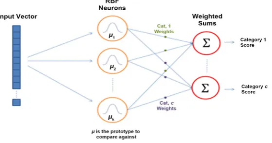
RBFN deals with attrubute/feature values that are clustered. The attribue values in a cluster are fitted with the radial basis function which is another name for Gaussian function. RBFN fuzzifies the attribute values in a cluster into the membership function values. Each RBFN neuron stores a cluster centre or centroid, which is initially taken to be one of the samples from the training set. When we want to classify a new input, each neuron computes the Euclidean distance between the input and its centroid and computes the membership function using the standard deviation or width of the Gaussian function. The output of the RBFN is a weighted sum of the membership function values as shown in Figure 1. In this µi denotes the ith membership

function (MF) of a neuron. The MF vector is of size k and each value of this vector is multiplied with the output weight and then summed up to get the computed output.

2.1. The Derivation of the Model of RBFN

We will derive an input-output relation underlying the architecture of RBFN in

Figure 1 in which prototype refers to the cluster centre. In this architecture there are two phases. The first phase is fuzzification and second phase is regression. For the fuzzification let us assume a cluster consisting of feature vectors of dimension k. Let ith_feature_X_ui_{in this vector X}_u_{be fuzzified using the i}th membership function µi and u stands for uth input vector-output pair. Thus

we have k fuzzy sets. Here we have as many neurons as the number of the input feature values. We don’t require any equation for this phase. In the regression phase we employ Takagi-Sugeno-Kang fuzzy rule [8] on k-input fuzzy sets and one output as:

If Xu1 is A1 and Xu2 is A2 and ∙∙∙ Xuk is Ak then

0 1 1 2 2

u u u k uk

Y = +b b X +b X + + b X (1)

where the fuzzy set Ai=

{

Xui,Pui

}

|u=1,, ;m i=1, 2,,k. Now substituting

the fuzzified inputs, i.e. Pui=µi

( )

Xui , for the inputs we get

0 1 1 2 2

u u u uk

Y =b +b P +b P + + b (2)

This equation is valid if there is one class. We now extend this equation to the multi-class case. We feed the input vector of size k denoted by Xu and the neurons compute the membership function values Puj. Let the number of classses be c. The regression equation that computes the outputs Yl in multi-class is framed as:

0 1 1 2 2 ; 1, ,

l l l u l u kl uk

Y =w +w P +w P + + w P l=  c (3)

where we have replaced the weight vector {bi} by the weight matrix {wil} to account for multi-class. This is the governing equation for the architecture in

Figure 1. The calculation of the output weights is deferred to Section III. The

(4)

[image:4.595.235.515.74.221.2]

DOI:10.4236/jmp.2019.1013100 1508 Journal of Modern Physics Figure 1. Architecture of RBFN.

2.2. Procedure for Learning of Weights

Consider first the problem of Iris flower recognition. In this we have 4 features. That is each feature vector is 4 dimensional. Assume that these are clustered into say, 3. It means that each cluster contains some number of feature vectors. According to the fuzzy set theory, we can form 4 fuzzy sets in each cluster corresponding to four features. Now each fuzzy set is defined by its attribute values and their membership function values. As we are using clustering, we can obtain mean values as well as scaling factors that are functions of variances involved in MFs of the fuzzy sets resulting from clustering. Our attempt is to focus on learning of weights.

Let us assume that we are feeding each feature vector of a cluster. Then we will have four neurons that convert four feature values of the feature vector into four membership function values. Then these membership values will be summed up. As we have assumed three clusters for one class (each flower type of Iris), this procedure is repeated on all feature vectors of the remaining two clusters. By this, we get three sumswhich will be multiplied with three weights (i.e. forming one weight vector) and the weighted sum is the computed output that represents one class.

The above procedure is repeated for the other three classes and the three weight vectors so obtained correspond to the remaining three flower types. There will also be three weighted sums called the computed outputs. In this paper, we are concerned with one cluster per class for simplicity.

3. Training of RBFN

The training process for RBFN consists of finding the three sets of parameters: the centrods of clusters, scaling parameters for each of the neurons of RBFN, and a set of the output weight vectors between the neurons and the output nodes of RBFN. The approaches for finding the centriods and their variances are discussed next.

3.1. Cluster Centrods

(5)

selection of centroids, Clustering based approach and Orthogonal Least Squares (OLS). We have selected the K-means clustering for the computation of centroids of clusters or cluster centres from the training setr. Note that this clustering method partitionsn observations into K number of clusters such that each observation having its value closest to the cluster centre belongs to that cluster.

3.2. Scaling Parameters

Camped with the centoid of each cluster, the variance is computed as the average distance between all points in the cluster and the centrod.

(

)

2

1

1 m

i u Xui Ci

m

σ =

∑

₌ − ₍₄₎

Here, Ci is the centroid of ith cluster, m is the number of training samples

belonging to this cluster, Xui is the uth training sample in the ith cluster. Next we use 2

i

σ _{to compute the scaling parameters denoted by} _i 1₂

i

β σ = _.

3.3. Output Weights

In the literature, there are two popular methods for the determination of the output weights: one learning method called gradient descent [11] and another computational method called pseudo inverse [12] [13]. As gradient descent learning has problems of slow convergence to local minima, we embark on a new learning algorithm called JAYA. Prior to using JAYA for learning the parameters of RBFN, we will discuss how the weights can be determined by Pseudo-inverse (PINV) method.

Consider an input vector which is generally a feature vector of some dimension n. When all the feature vectors are clustered, we will have C number of clusters (Note that c denotes the number of classes). In some datasets such as Iris dataset, we can easily separate out all the feature vectors belonging to each class of one flower type. Thus the feature vectors belonging to a class form a cluster. Out of these feature vectors some are selected for training and the rest for testing.

Let

{

Xu,Zu

}

;u=1,,m be the set of feature vectors with each feature vector

having the size of n, i.e. k u

X ∈R with target, Zul∈Rc, and Puj =µi

( )

Xuj be

the membership function of the jth_{basis radial function}

j

µ with the uth_feature vector. Xuj is the jth component of the feature vector Xu and Zul is the lth target output. Note that this formulation is meant for one cluster per one class. After the fuzzification of Xuj into Puj, we can form a matrix P by taking u=1,,m;

1, 2, ,

j=  k. The matrix Q is written as

P11 P12 ∙∙∙ P1k

P21 P22 ∙∙∙ P2k

.. ∙∙∙ ..

(6)

As we have Wl =

[

w w1l, 2l,,wkl

]

; Z ll; =1, 2,,c; Z =

[

Z Z1, 2,,Zc

]

. Let

us denote Q=

[

P P1, 2,,Pm

]

with Pu=

[

Pu1,Pu2,,Puk

]

and

[

1, 2, , k

]

W = W W W . The objective function to be minimized is given by:

(

)

2

, ,

f W Q Z = W Q∗ −Z (5)

where Y =W Q∗ with Y =

[

Y Y1, 2,,Yc

]

as per Equation (3). The solution to

the above equation lies in the assumption that be Y =W Q∗ =Z which leads to W =Q Z+ where Q+ denotes the pseudo inverse matrix of Q, defined as follows:

(

_T

)

1 _T

0

lim Q Q _n

Q I Q

α γ

− →

+ ₌ ₊ ₍₆₎

where Ik is the k-dimensional unity matrix and γ is a small positive constant.

The pseudo inverse

(

_T

)

1 _T

Q+= Q Q − Q exists if (QTQ) is nonsingular. After

calculating the weights at the output layer, all the parameters of RBFN with its 3-layered architecture in Figure 1 can be determined.

4. Learning of the Output Weights by JAYA

We will now discuss JAYA algorithm to be used for learning the parameters of RBFN.

Description of the JAYA Algorithm

It is a simple and powerful learning method for solving the constrained and unconstrained optimization problems. As mentioned above JAYA algorithm is the offshoot of Teacher-Learner Based Optimization (TLBO) algorithm proposed in [14][15]. This needs only the common controlling parameters like population size and number of iterations. The guidelines for fixing these parameters can be seen in [15]. Here we have fixed the population size as 10 and the number of iterations as 3000.

Let f W Q Z

(

, ,

)

be the objective function to be minimized. Let the best

candidate be the one associated with the least value of the function (i.e.

(

, ,

)

best

f W Q Z ) and the worst candidate is the one with the highest value of the

function (i.e. fworst

(

W Q Z, ,

)

) in all the candidate solutions. We choose B to

stand for the weights W when the cluster centres and scale parameters are found separately. In case we use to learn all the parameters, B includes the cluster centres, scaling parameters and the output weights, i.e. B=

[

C, ,β W

]

.

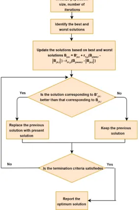
At any run of the algorithm, assume that there are ‘j’ design variables and ‘k’ candidate solutions and ‘i’ iterations. So to fit B into the JAYA algorithm, it is denoted by Bj k i, , which is the value of the jth variable of the kth candidate during the ith_iteration.

, ,

j k i

B is updated to B_{j k i}′_{, ,} during the iteration as,

(

)

(

)

, , , , 1, , , , , , 2, , , , , ,

j k i j k i j i j best i j k i j i j worst i j k i

B′ =B +r B − B −r B − B (7)

where Bj best i, , is the value of the jth variable for the best candidate, Bj worst i, , is the value of the jth_{variable for the worst candidate at i}th_{iteration and}

1, ,j i

r and

2, ,j i

r are the two random numbers in the range 0 to 1 for the jth variable at the ith

(7)

to the best solution whereas the term r2, ,j i

(

Bj worst i, , − Bj k i, ,

)

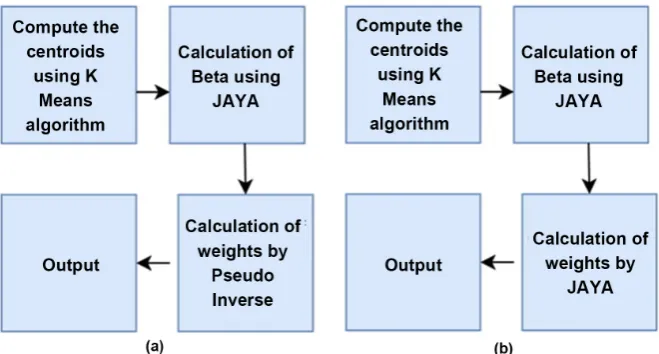
indicates the tendency to avoid the worst solution. B′j k i, , is accepted if its function value is better than that of Bj k i, , . All the accepted function values at the end of iteration are retained and these values become the input to the next iteration. The flowchart of JAYA algorithm is shown in Figure 2. Unlike TLBO algorithm that has two phases (i.e. teacher and learner), JAYA algorithm has only one phase and it is comparatively simpler to apply. Rao et al. [16] have used TLBO algorithm in the machining processes. A tea-category identification (TCI) system is developed in [17] and it uses a combination of JAYA algorithm and fractional Fourier entropy on three images captured by a CCD camera. In two studies involving heat transfer and pressure drop, i.e. thermal resistance and pumping power, two objective functions are used to ascertain the performance of the micro-channel heat sink. Multi-objective optimization aspects of plasma arc machining (PAM), electro-discharge machining (EDM), and micro electro-discharge machining (μ-EDM) processes are investigated in [18]. These processes are optimized while solving the multi-objective optimization problems of machining processes using MO-JAYA algorithm.

There are three learning parameters, viz., the cluster centers Ci, the scaling parameters (βi) and the output weights W between the hidden and output

layers. The learning of these parameters is depicted in Figure 3. The first parameter is found using K-means clustering algorithm.

We make use of JAYA algorithm for learning the second parameter, βi. The

weights are learned by optimizing the objective function using JAYA algorithm. The RBFN model so obtained can then be used for both classification and function approximation.

5. Design of Hanman Entropy Network

[image:7.595.208.538.513.690.2]

As the RBFN is not geared up to take care of the uncertainty in the input which may be an attribute or property value, we will make use of the Information set

(8)

[image:8.595.233.517.78.505.2]

DOI:10.4236/jmp.2019.1013100 1512 Journal of Modern Physics Figure 3. Flowchart of JAYA algorithm.

(9)

5.1. Definition of Information Set and Generation of Features Consider a fuzzy set constructed from the feature values {Xuj} termed as the Information source values and their membership function values which we take as the Gaussian function values {Puj}. If the information source values do not fit the Gaussian function, we can choose any other mathematical function to describe their distribution. Thus each pair (Xuj, Puj) consisting of information source value and its membership value is an element of a fuzzy set. Puj gives the degree of association of Xuj and the sum of Puj values doesn’t provide the uncertainty associated with the fuzzy set. In the fuzzy domain, only Puj is used in all applications of fuzzy logic thus ignoring Xuj altogether. This limitation is eliminated by applying the information theoretic entropy function called the Hanman-Anirban function [22] to the fuzzy set. This function combines the pair of values Xuj and Puj into a product termed as the information value given by

uj uj uj

H =X P (8)

The above relation owes its derivation to the non-normalized Hanman-Anirban entropy function expressed as

(

3 2

)

1 e

uj uj uj

aX bX cX d n

uj j

H=

∑

₌ X − + + + (9)

where a, b, c and d are the real-valued parameters. In this equation normalization by n is not needed as the number of attributes is very small (less than 10 in the databases used) but needed if the value of H exceeds more than 1.

With the choice of parameters: a=0, 1₂

2

b

σ

= _, 2 ₂

2

X c

σ

= − _and 2₂

2

X d

σ

=

where X is the mean value and σ2 is the variance of the information source

values Xuj , the exponential gain function is converted into the Gaussian

function Pu. As a result, Equation (9) is modified to

1

n uj uj j

H =

∑

₌ X P (10)

The set of information values constitutes the information set denoted by

{ } {

Huj X Puj uj

}

= =

 whereas the corresponding fuzzy set is simply {Xuj, Puj}. Consider another entropy function called Mamta-Hanman entropy function [20]

which is a generalized form of Hanman-Anirban entropy function, expressed as:

(

)

e cXuj d

MH uj

H X

ρ γ

α − +

=

∑

₍₁₁₎

Substituting c 1

σ

= _and d X

σ

= − _{in (11) modifies} H_MH to the following:

1

n

MH j uj uj

H =

∑

₌ X Gα (12)

where Guj is the generalized Gaussian function given by

e uj X X uj G ρ γ σ  −    −      =

(10)

Assuming each information value as a unit of information, we can derive several modified information sets. For instance application of sigmoid function on

uj uj

X Gα leads to

1

1 e uj uj

n

j _{X G}

S ₌ _α

−

=

+

∑

(13)

In Equations (9)-(13) the information values are the ones inside the summation sign. Thus a family of information forms can be deduced from both Hanman-Anirban and Mamta-Hanman entropy functions for dealing with different problems. For the derivation of different forms of H and HMH the readers may refer to [19] and [21] respectively.

5.2. The Hanman Transform and its Link to Intuitionistic Set This is a higher form of information set. To derive this transform, we have to consider the adaptive form of Hanman-Anirban entropy function in which the parameters in the exponential gain function are taken to be varaibles. Assuming

0

a= = =b d and c=P_uj in (9) we obtain the Hanman Transform [21]:

1 e 1 e

uj uj uj

n X P n H

T j uj j uj

H =

∑

₌ X − =

∑

₌ X − (14)

Note that the exponentional gain function in (14) is a function of the information value. This transform acts as an evaulator of information values based on the information values obtained on them. The higher form of information set

{

e Huj

}

uj

X − isrecursive because r.h.s of (14) can be rewritten as

(

)

( )

e Hujold

uj uj

H new =X − (15)

An interesting result termed as Shannon transform emerges from Hanman transform by changing the substitution such that d = −1 instead of 0 in (9) and then simplifying the resulting exponential function as follows:

1

1 e 1 log

uj

n H n

Sh j uj j uj uj

H =

∑

₌ X − =

∑

₌ X H (16)

Let us consider the adaptive Hanman-Anirban entropy function involving the membership functions alone. Then we have

( ) ( ) ( ) ( )

(

_. 3 _. 2 _. _.

)

1 e

uj uj uj

a P b P c P d n

uj j

H =

∑

₌ P − + + + (17)

This gives the uncertainty in the membership function values. This is useful when a mathematical function describing the information source values is not appropriate thus leading to error in the fuzzy modeling. Now with a particular substitution of values for a

( )

. =b

( )

. =d

( )

. =0 and c

( )

. =Xuj. Equation (14)

takes the form

1 e

uj

n H

T j uj

H =

∑

₌ P − (18)

(11)

(

)

( )

e Hujold

uj uj

P new =P old − (19)

On the lines of derivation of (19), we can have another derivation from (11) as follows:

(

)

( )

e Hujold

uj uj

P new =Pα old − (20)

This is a useful relation becuase it can be used to make RBFN adaptive by changing the membership function. At this juncture we can make an interesting connection between the modified membership function in Equation (19) and hesitancy function in the Intuitionistic fuzzy set [23]. The hesitancey function is defined as follows:

1

uj uj ucj

h = −P −P (21)

where Pucj = −1 Puj, the complemetary of Puj. The hesitancy function reflects the

uncertainty in the modeling of Puj and Pucj. As Equation (19) bestows the way to evaluate Puj, we can use the new values of Puj and Pucj in determining the updated value of huj as follows:

(

)

1

(

)

(

)

uj uj ucj

h new = −P new −P new (22)

where

(

)

( )

e Hucj( )old

ucj ucj

P new =P old − and H_ucj =X P_uj _ucj . We can use this

hesitancy function for the design of a new network in future.

5.3. Properties ofInformation Set

We will now present a few useful properties of Information set.

1) In the information set, the product of the complementary membership function value and the information source value gives the complementary information value.

2) Information values are natural variables just as signals received by biological neuron from visual cortex after modification by synapse.

3) The information values can be modified by applying various functions to provide effective features.

4) Higher form of information values like Hanman Transform provides a better representation of the information source values.

5) The fuzzy rules can be easily aggregated using the information set concept.

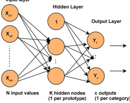
5.4. The Architecture and Model of Hanman Entropy Network We will now discuss the architecture of HEN in Figure 4.

The architecture of HEN is the same as that of RBFN but for the function ϕi,

which assumes the specified form of an entropy function of the input. In HEN each n-input vector needs to be categorized into any one of “c” classes. The ith function denoted by ϕi converts all the values of the input vector into the

entropy function values. This will be clear if we consider the Takagi-Sugeno-Kang fuzzy rule for multi-class case:

(12)

[image:12.595.263.480.77.249.2]

DOI:10.4236/jmp.2019.1013100 1516 Journal of Modern Physics Figure 4. The Architecture of HEN.

0 1 1 2 2

v v v u v u vn un

Y =b +b X +b X + + b X (23)

As mentioned above that at the fuzzification phase we replace bvj with Pvj and set Pv0 to 0 in (23) to get the neuron output as:

1 1 2 2 ; 1,

v u v u v

v P X P X P Xn un v

ϕ = + + + =  (24) On substituting Huj for the information values in (24) we get:

1 2 ; 1, 2, ,

v v vn

v H H H v k

ϕ = + + +_ = _ ₍₂₅₎ Thus the fuzzification phase in HEN is different from that of RBFN. In HEN the input feature vectors of size n are clustered into k clusters but in RBFN there is a single cluster for each feature of a feature vector. Each neuron in RBFN of

Figure 1 has only one radial basis function whereas each neuron in HEN has k

radial basis functions in Figure 4. So in Equation (25) k sums ϕ1 to ϕk will be

multiplied with the corresponding weights w1l to wkl to yield the lth output Yl in the regression phase as follows:

1

1 2 2

0 ; 1, ,

l l l l kl k

Y =w +w ⋅ +ϕ w ⋅ϕ + + w ⋅ϕ l=  c (26)

Here ϕ0=1 and ϕ=

[

1,ϕ ϕ1, 2,,ϕk

]

; Wl =

[

w0l,w1l,,wkl

]

. This is the

governing equation of Hanman Entropy Network in Figure 4. The objective function to be optimized by the JAYA + HEN combination is different. In view of this, the objective function becomes:

(

)

2

, _l, _l _l _l

f ϕW Z = W ∗ −ϕ Z (27)

Instead of µj in RBFN, we will now use ϕj in HEN. In the general case

j

ϕ can be taken as any relation linking the information source values to their membership function values. Thus, we can assume the following relations for this function:

{

uj uj

}

MH

j u X G

α

ϕ =

_∑

_or

S

1

1 e Xuj uj

u − αG

 

 

 

 

 + 

∑

or

{

}

T

e Huj

u

u X j

−

∑

or

{

log

}

_Sh

u Xuj Huj

(13)

where subscripts MH, S, T and Sh indicate Mamta-Hanman, Sigmoid, Hanman transform and Shannon transform respectively. Note that RBFN network simply responds to the pattern in the input vector but the Hanman entropy network responds not only to the pattern but also to the uncertainty associated with it.

6. Results of Case Studies

The experimentation is conducted on four datasets: IRIS, Wine, and Waveform from UCI repository and Signature dataset [24] in two phases. In the first phase, we have entirely dealt with the performance analysis of RBFN and in the second phase only with that of Hanman Entropy Network (HEN). We have split up our computations into two cases. In Case-1 which is applicable only to RBFN, the learning/computation of the output weights is delinked from the computation of centriods and scaling parameters. Next, we have employed two learning methods such as Genetic algorithm (GA) and Gradient Descent (GD) and one computational method called Pseudo inverse (PINV) for the weights and K-means clustering for the centriods and scaling parameters.

There is another combination, JAYA + PINV + RBFN wherein JAYA is used for learning scaling parameters and PINV is used for computing the output weights. Of course, the centroids are found by K-means clustering.

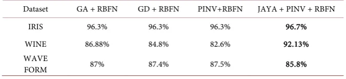
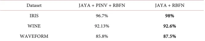
The notations GA + RBFN, GD + RBFN, PINV + RBFN and JAYA +P INV refer to the learning of weights of RBFN by Genetic Algorithm, Gradient descent, Pseudo-Inverse, JAYA + PINV combination respectively. The results of classification accuracy with these four methods GA, GD, PINV and JAYA + PINV along with RBFN are given in Table 1. The last combination gives the best results. Table 2 gives the comparison of JAYA + PINV + RBFN with JAYA + RBFN where the latter shows the best results.

A brief exposition on how to form fuzzy sets from which information sets are formed is the need of the hour. Assuming n feature types of an object, say, signature we form n fuzzy sets by collecting all the feature values of each feature type and fitting the radial basis function with the help of centroid (mean value of feature values) and scaling parameter (variance). Then conversion of this fuzzy set to information set is a simple matter.

The dataset-wise discussion of results follows the next.

[image:13.595.203.541.650.727.2]

IRIS dataset: This dataset consists of three classes with 50 samples for each class. There are four attributes for each sample. These are: sepal length, sepal

Table 1. A comparison of the Classification accuracy of RBFN using several learning methods on different datasets.

Dataset GA + RBFN GD + RBFN PINV+RBFN JAYA + PINV + RBFN

IRIS 96.3% 96.3% 96.3% 96.7%

WINE 86.88% 84.8% 82.6% 92.13%

WAVE

(14)

[image:14.595.207.541.102.170.2]

DOI:10.4236/jmp.2019.1013100 1518 Journal of Modern Physics Table 2. A comparison of the Classification accuracy of RBFN using JAYA for the learning of all parameters.

Dataset JAYA + PINV + RBFN JAYA + RBFN

IRIS 96.7% 98%

WINE 92.13% 92.6%

WAVEFORM 85.8% 87.5%

width, petal length and petal width all in cms. The classes are: Setosa, Versicolour and Virginica. It may be noted that GA, GD and PINV learning methods yield the classification accuracy of 96.3% when used for learning the weights of RBFN by classifying 144 instances out of 150. However, the combination symbolized by JAYA + PINV + RBFN gives the accuracy of 96.7% which uses 1) JAYA to learn the scaling parameters and 2) PINV to learn the weights of RBFN. This is the best result among all the results obtained on this dataset by the methods compared.

WINE dataset: The dataset consists of three classes with class 1, class 2, class 3 having 59, 71, 48 samples repectively. Each sample has 13 attribultes that include Alcohol, Malic acid, Ash, Alcalinity of ash, Magnesium, Total phenols, Flavanoids, Nonflavanoid phenols, Proanthocyanins, Color intensity, Hue, OD280/OD315 of diluted wines and Proline. The classification accuracies of 84.8% and 82.6% are achieved with GD and PINV respectively when these are used for the determination of the output weights of RBFN whereas GA + RBFN combination gives an accuracy of 86.88%. However, the best accuracy of 92.13% is achieved with JAYA-RBFN combination.

WAVEFORM dataset: The dataset consists of 5000 samples with each sample comprising 22 attributes. Each class is generated from a combination of 2 out of 3 “base” waves and each instance is generated by adding noise (mean 0, variance 1) to every attribute. RBFN classifies 4350 instances correctly out of 5000 instances with an accuracy of 87% with GA. The weights of RBFN computed using GD and PINV yield the best accuracies of 87.4% and 87.5% respectively but with JAYA + RBFN combimation the accuracy comes down to 85.8% in

Table 2.

As can be seen from the results, the efficiency of the classification task increases when we use JAYA algorithm even for learning the weights of the network in comparison to learning the scaling parameters of the membership function. When the concept of information set is incorporated into our approach, the output is computed as Weights*Information values, i.e. Wl∗ϕ. If

the parameter vector, B also includes the centrods and the scaling parameters in addition to the weights then these parameters modify Pu indirectly. Then we will write ϕ ϕ′ =

(

C,β

)

. Accordingly the objective function is modified as:

(

)

2

, _l, _l _l _l

f ϕ′W Z = W∗ϕ′−Z (29)

(15)

[image:15.595.207.541.89.124.2]

DOI: 10.4236/jmp.2019.1013100 1519 Journal of Modern Physics Table 3. A comparison of Verification accuracy on Signature dataset.

Dataset JAYA + PINV + RBFN JAYA + RBFN HEN

SVC2004 90.7% 99.6% 99.8%

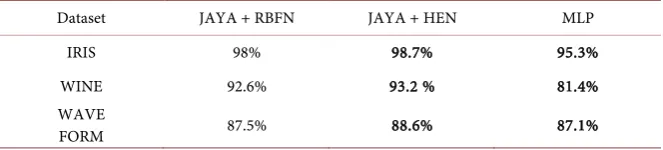
Table 4. Comparison of Classification accuracy.

Dataset JAYA + RBFN JAYA + HEN MLP

IRIS 98% 98.7% 95.3%

WINE 92.6% 93.2 % 81.4%

WAVE

FORM 87.5% 88.6% 87.1%

(

)

2

, ,

i l l l i l

f P W Z′ = W ∗P′−Z (30)

Applying JAYA on (29) and (30) learns B.

SIGNATURE dataset: This dataset (SVC2004) in [24] has been used for a competition and it consists of 20 skilled forgeries and 20 genuine signatures of 40 users. Each signature in the dataset is represented as a sequence of points containing X and Y co-ordinates, time stamp and pen status (pen up or down) along with the additional information like azimuth, altitude and pressure. The text file contains a sequence of 7-dimensional measurements (feature types) for each signature. Our previous work on signature verification using Information set features on this dataset shows the effectiveness of these features [25]. We have used JAYA for learning both scaling parameters and the output weights of Hanman Entropy network (HEN) just as in JAYA + RBFN combination. The results of classification accuracy with JAYA + HEN are slightly better than those of JAYA + RBFN. But with JAYA + PINV + RBFN combination the results are very poor as shown in Table 3. The power of Hanman Entropy network can only be realized when the dataset is very large.

On conducting tests on three datasets as shown in Table 4, we find that the performance of JAYA + RBFN combination is somewhat inferior to that of JAYA + HEN combination on three datasets (Iris, Wine and Waveform) but the performance of Multi-layer perceptron (MLP) network is the worst. The use of high level information set features may help improve the performance of JAYA + HEN.

7. Conclusions

[image:15.595.208.540.158.233.2]

(16)

As HEN is based on information set theory that caters to uncertainty representation; there is so much flexibility in the choice of information forms. This advantage is missing in RBFN where only the membership function values rule the roost. The only silver lining with RBFN is that we can use Type-2 fuzzy sets where the membership function values can be varied by changing the variance parameter of Gaussian membership function.

The present work opens up different directions to change the information at the hidden neurons of HEN.

Acknowledgements

The authors acknowledge the comments of anonymous reviewers, which helped improve the paper.

Conflicts of Interest

The authors declare no conflicts of interest regarding the publication of this paper.

References

[1] Rumelhart, D.E., Hinton, G.E. and Williams, R.J. (1986) Nature, 323, 533-536. https://doi.org/10.1038/323533a0

[2] Moody, J. and Darken, C.J. (1989) Neural Computation, 1, 281-294. https://doi.org/10.1162/neco.1989.1.2.281

[3] Hecht-Nielsen, R. (1987) Applied Optics, 26, 4979-4984. https://doi.org/10.1364/AO.26.004979

[4] Bullinaria, J.A. (2015) Radial Basis Function Networks: Algorithms, Neural Com-putation: Lecture 14. http://www.cs.bham.ac.uk/~jxb/INC/l14.pdf

[5] Poggio, T. and Girosi, F. (1990) Proceedings of IEEE, 78, 1481-1497. https://doi.org/10.1109/5.58326

[6] Grover, J. and Hanmandlu, M. (2018) Applied Intelligence, 48, 3394-3410. https://doi.org/10.1007/s10489-018-1154-x

[7] Rao, R.V. (2016) International Journal of Industrial Engineering Computations, 7, 19-34.https://doi.org/10.5267/j.ijiec.2015.8.004

[8] Jang, J.S.R., Sun, C.T. and Mizutani, E. (2009) Neuro-Fuzzy and Soft-Computing: A Computational Approach to Learning and Machine Intelligence. PHI Learning Pri-vate Limited, New Delhi.

[9] Orr, M.J.L. (1995) Neural Computation, 7, 606-623. https://doi.org/10.1162/neco.1995.7.3.606

[10] Xie, T.T., Yu, H. and Wilamowski, B. (2011) Comparison between Traditional Neural Networks and Radial Basis Function Networks. Industrial Electronics (ISIE).

IEEE International Symposium, Gdansk, 27-30 June 2011, 1194-1199.

[11] Parappa, S.N. and Pratap Singh, M.P. (2013) International Journal of Advancements

in Research & Technology, 2, 112-125.

(17)

https://doi.org/10.1016/S0893-6080(01)00027-2

[14] Rao, R.V. and Patel, V. (2013) Scientia Iranica, 20, 710-720. https://doi.org/10.1016/j.scient.2012.12.005

[15] Rao, R.V., Savsani, V.J. and Vakharia, D.P. (2011) Computer-Aided Design, 43, 303-315.https://doi.org/10.1016/j.cad.2010.12.015

[16] Rao, R.V. and Kalyankar, V.D. (2012) Journal of Materials and Manufacturing

Processes, 27, 978-985.https://doi.org/10.1080/10426914.2011.602792

[17] Zhang, Y., Yang, X., Cattani, C., Rao, R.V. and Wang, S. (2016) Entropy, 18, 77. https://doi.org/10.3390/e18030077

[18] Rao, R.V., Rai, D.P., Ramkumar, J. and Balic, J. (2016) Advances in Production

En-gineering & Management, 11, 271-286.https://doi.org/10.14743/apem2016.4.226

[19] Hanmandlu, M. (2013) Expert Systems with Applications, 40, 6478-6490. https://doi.org/10.1016/j.eswa.2013.05.020

[20] Hanmandlu, M. (2014) Engineering Applications of Artificial Intelligence, 36, 269-286.https://doi.org/10.1016/j.engappai.2014.06.028

[21] Sayeed, F. and Hanmandlu, M. (2017) Knowledge and Information Systems, 52, 485-507.

[22] Hanmandlu, M. and Das, A. (2011) Defence Science Journal, 61, 415-430. https://doi.org/10.14429/dsj.61.1177

[23] Xu, Z. (2007) IEEE Transactions on Fuzzy Systems, 15, 1179-1187. https://doi.org/10.1109/TFUZZ.2006.890678

[24] Chang, W. and Shin, J. (2008) DPW Approach for Random Forgery Problem in Online Handwritten Signature Verification. 4th International Conference on

Net-worked Computing and Advanced Information Management, Gyeongju, 2-4

Sep-tember 2008, 347-352.https://doi.org/10.1109/NCM.2008.118