ABSTRACT
YURGEC, MATTHEW JOSEPH. A Rheological Analysis of Shear on a Model Emulsion System. (Under the direction of Dr. Christopher Daubert.)
Shear work and shear power intensity are two rheological terms developed to quantify the amount of shear energy that a fluid is exposed to during processing. In this study, the effect of shear work and shear power intensity on a model corn oil-in-water emulsion was evaluated. Results revealed that when the model emulsion was
homogenized at a constant shear work, the median particle size was statistically identical even though the homogenization pressures or shear power intensities required to achieve that shear work level were different. Median particle size was considered a function of the shear work input and the surfactant concentration, and a simple mathematical model using a power function was formulated. Median particle size decreased initially as shear work was applied, but at some critical value, the median particle no longer reduced, maintaining a constant level. Using a statistical piece-wise linear or “hockey-stick” model, an isolated critical value for shear work and the corroborating median particle size was found with a fit accounting for greater than 90% of the variability.
Viscosity results from this study showed that Newtonian viscosities were not significantly different when shear work or shear power intensity were different. There was some evidence that increasing the shear power intensity increased the viscosity slightly, but not significantly. In this study, surfactant concentration was critical to median particle size.
A Rheological Analysis of Shear on a Model Emulsion System
by
Matthew Joseph Yurgec
A thesis submitted to the Graduate Faculty of North Carolina State University
in partial fulfillment of the requirements of the Degree of
Master’s of Science
Food Science Raleigh, NC
2009
APPROVED BY:
__________________________ _________________________ E. Allen Foegeding, Ph.D. Mitzi Montoya, Ph. D. Co-Advisor
DEDICATION
I would like to dedicate this thesis to my wonderful girlfriend, Katie Wagner. You have been, without a doubt, the most supportive person during my time here at N.C. State. I can’t believe it has been two years since we were saying our goodbyes at a Manhattan street corner as I made my final preparations for my move to North Carolina. I didn’t think anything could top going with you to the Red Lion, Panchito’s or the Caves in NY/NJ, but in NC we found Mac’s, Napper Tandy’s trivia, and Bloomsbury. I am so fortunate that I have you and I am so appreciative of you for moving away from your family and friends to join me here in North Carolina. You have provided me with countless meals and have kept me from ever having to open a can of tuna or a box of ramen noodles. You kept me from slacking off and kicked my rear end when it was time to do research, study, or hit the gym. Thank you for the countless hours you listened to me worrying about a test, a class project, my thesis, the homogenizer, and most
BIOGRAPHY
Matthew Joseph Yurgec was born on August 5, 1983 in Pittsburgh, PA and grew up in South Park, PA. He graduated from South Park High School in 2001 and entered college at Penn State University in August of 2001, where he majored in Food Science. While at Penn State, Matthew was an active member of the Penn State Food Science Club, which he was president of during his senior year. Matthew also was a Resident Assistant during his junior year in Simmons Hall and enjoyed playing golf as a member of the Penn State Golf Club. During his matriculation at Penn State, he had two
ACKNOWLEDGMENTS
- To Dr. Daubert for being a wonderful adviser. You helped me become a much better scientist and helped me “see the forest through the trees”. You also showed patience every week as I tried to learn how to be a writer and a scientist. Every weekly meeting helped set my mind straight and allowed me to keep moving forward with my research. Most importantly, thanks for our in-depth discussion of Penn State football (among other sports). WE ARE…..PENN STATE. - To Mom and Dad for providing me with support throughout graduate school.
Without your emergency trip to PNC, my belongings may forever have been in the possession of the moving company. I also really appreciate the groceries and gas that you have provided me, the flights home you paid for, and the occasional meal that you gave me.
- To my sister Alexis and brother-in-law Mike for giving me a place early on where there were people I knew. Thank you for letting me stay at your place that first weekend when my other option would have been sleeping on the floor in an empty apartment. Oh yeah, thanks for all those meals, too.
- To Sharon Ramsey, the person who keeps the Rheology Lab running and so many other activities afloat. Thanks for your help with my research, the “cheese
project”, and helping me with TA’ing last fall. You are certainly one person who deserves a long vacation.
- To Dr. Foegeding for being a world-class teacher and scientist. Your class was extremely useful and it gave me a new understanding of the world of food and colloidal chemistry. You gave me an appreciation for the skills that are required for being a thorough and thoughtful scientist.
- To Dr. Mitzi Montoya, Minor Thesis Advisor for being part of my committee. Thank you for your help in selecting classes for my Minor in Business
Administration. It was a pleasure getting to know you.
- To Dr. Jason Osborne from the N.C. State Department of Statistics for his help with the statistical analysis involved in this project.
- To Dr. Jim Steffe for helping to develop the rheological shear values that much of this project revolves around.
TABLE OF CONTENTS
LIST OF TABLES ... viii
LIST OF FIGURES ... ix
LITERATURE REVIEW ... 1
1.1. Shear-Sensitivity of Fluids... 2
1.2 Overview of Rheology... 3
1.2.1 Definition of Rheology ... 3
1.2.2 Stress and Strain... 4
1.2.3 Fluid Rheology... 5
1.2.4 Rotational Viscometry ... 7
1.2.5 Pipeline Design Calculations ... 9
1.3 Rheological Values for Shear Energy... 10
1.3.1 Shear Work: Quantification of shear history ... 11
1.3.2 Shear Power Intensity ... 12
1.3.3 Differences between Shear Work and Power Intensity ... 14
1.4 Emulsions... 17
1.4.1 Water: Continuous Phase... 18
1.4.2 Oil: Dispersed Phase ... 19
1.5 Emulsifiers ... 21
1.5.1 Surfactants... 22
1.5.1.1 Critical Micelle Concentration... 26
1.5.1.2 Cloud point... 26
1.5.2 Tween-series surfactants... 27
1.6 Emulsion Formation... 29
1.6.1 Homogenization... 31
1.6.1.1 Droplet Disruption ... 33
1.6.1.2 Droplet Coalescence ... 35
1.7 Emulsion Stability/Instability ... 36
1.7.1 Creaming and Sedimentation... 38
1.7.2 Coalescence... 40
1.7.3 Flocculation... 42
1.7.4 Phase Inversion ... 43
1.7.5 Ostwalt Ripening ... 44
1.8 Emulsion Rheology... 45
1.9 Conclusion ... 50
QUANTIFICATION OF SHEAR EFFECTS AND IDENTIFICATION OF
CRITICAL SHEAR VALUES OF A MODEL EMULSION SYSTEM ... 55
2.1 Introduction... 56
2.1.1 Background ... 56
2.1.2 Shear Work and Shear Power Intensity Defined ... 59
2.2 Materials and Methods... 63
2.2.1 Coarse Emulsion Preparation... 63
2.2.2 Homogenization... 64
2.2.3 Particle Size Analysis ... 64
2.2.4 Rheological Measurements... 66
2.2.5 Calculation of Shear Work (Ws) ... 66
2.2.6 Experimental Design Matrix... 67
2.2.7 Shear Work Critical Limit Determination ... 69
2.2.8 Mathematical Model of Data ... 69
2.3 Results and Discussion: ... 70
2.3.1 Particle Size Results... 70
2.3.1.1 Particle size as a function of shear work and power intensity ... 71
2.3.1.2 Median Particle Size as only Shear Work is Increased... 76
2.3.1.3 Median Particle Size at Constant Shear Work ... 79
2.3.1.4 Median Particle Size Response... 82
2.3.1.5 Statistical Description of Data ... 85
2.3.1.6 Critical Values for Shear Work... 85
2.3.1.7 Formulation and Testing of a Mathematical Model ... 89
2.3.2 Rheological Characteristics Results... 94
2.4 Conclusion ... 100
2.5 References... 103
EFFECT ON EMULSION PROPERTIES OF THE POSITIONING OF SHEAR DURING A HOMOGENIZATION PROCESS... 105
3.1 Introduction... 106
3.2. Materials and Methods... 109
3.2.1 Coarse Emulsion Preparation... 109
3.2.2 Homogenization... 109
3.2.3 Particle Size Analysis ... 111
3.2.4 Rheological Measurements... 112
3.3 Results and Discussion ... 113
3.3.1 Particle Size Results... 113
3.3.2 Rheology Results ... 115
3.4 Conclusion ... 116
BUSINESS IMPLICATIONS... 120
4.1 Shearing Problems in Food Industry... 121
4.2 Discarding or Recalling Products ... 121
4.3 Under-quality Products and Consumer Acceptance ... 122
4.4 Solutions to Shear Damaged Products... 123
4.5 Implementing the Solution... 125
4.6 Implementation Costs ... 125
4.7 Benefits ... 126
4.8 References... 127
CONCLUSIONS ... 128
APPENDICES ... 135
APPENDIX A ... 136
APPENDIX B ... 137
LIST OF TABLES LITERATURE REVIEW
Table 1.1: Variations of the Herschel-Bulkley model ... 7
Table 1.2: Shear work, shear power intensity and volume calculations for a typical System. ... 13
Table 1.3: Common surfactants and their associated HLB values. ... 25
Table 1.4: The action and type of emulsion formed at various HLB values. ... 26
Table 1.5: Properties of Tween series surfactants ... 29
QUANTIFICATION OF SHEAR EFFECTS AND IDENTIFICATION OF CRITICAL SHEAR VALUES OF A MODEL EMULSION SYSTEM Table 2.1: Shear work, shear power intensity, and volume calculations for a typical system ... 61
Table 2.2: Shear work values (MJ/kg) at each tested homogenization parameter... 68
Table 2.3: Identification of inflection points for shear work and minimum particle size reached at each Tween 20 surfactant concentration (w/w). ... 89
Table 2.4: Testing of mathematical model using random homogenization settings to achieve random shear workS and surfactant concentrations ... 92
Table 2.5: Comparison of models predicting particle size of 0.2% Tween 20 emulsions at 1 pass. ... 94
Table 2.6: Middle 68% of data range in particle size distributions. ... 100
EFFECT ON EMULSION PROPERTIES OF THE POSITIONING OF SHEAR DURING A HOMOGENIZATION PROCESS Table 3.1: Particle size results after first and second pass for each sample... 114
Table 3.2: Newtonian viscosity results after each pass is completed. ... 116
APPENDICES APPENDIX A: Complete table of median particle size results ± 1 st. dev... 136
APPENDIX B: Complete listing of Newtonian viscosities for sample treatments with 1 standard deviation... 137
LIST OF FIGURES LITERATURE REVIEW
Figure 1.1: a) Normal stress when force is applied perpendicular to surface; b) Shear stress when force is applied tangentially to surface... 4 Figure 1.2: Comparison of shear work and shear power intensity ... 15 Figure 1.3: From Tcholakova et al, linear relationship between particle size (ln
d32) and energy dissipation (ln pQ/Vs). ... 17 Figure 1.4: Emulsifier interaction at an oil/water interface... 22 Figure 1.5: Drawing of surfactant structures: I-anionic (sodium dodecyl sulfate);
2-cationic (dodecyltrimethylammonium bromide); and 3-non-ionic [n-dodecyl tetra (ethylene oxide)]... 23 Figure 1.6: Structure of Tween 20... 28 Figure 1.7: Description of Fg and Ff forces that drive stokes law... 39 Figure 1.8: Depiction of coalescence: 1) Droplets approach and collide with each
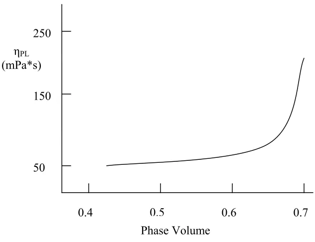
other, 2) Collision force is great enough to disrupt membrane, or there is insufficient emulsifier coverage and the droplets stick to one another, 3) Coalescence occurs, with two smaller droplets becoming one larger droplet. ... 41 Figure 1.9: Viscosity increase as phase volume fraction is increased, where ηpL
is relative viscosity of emulsion to pure continuous phase... 47 Figure 1.10: Viscosity of petroleum-in-oil emulsion under a shear stress ramp .. 48 QUANTIFICATION OF SHEAR EFFECTS AND IDENTIFICATION OF
CRITICAL SHEAR VALUES OF A MODEL EMULSION SYSTEM
Figure 2.1: Comparison of shear power intensity and shear work for two similar tanks with equal volumes of product. ... 63 Figure 2.2: Median particle size as pressure is increased at various number of
passes. ... 72 Figure 2.3: Median particle size as Tween 20 surfactant concentration was
increased at selected shear work levels... 75 Figure 2.4: Median particle size as the number of passes is increased at various
pressure settings... 77 Figure 2.5: Median Particle size using different homogenization treatments to
reach the same shear work value ... 80 Figure 2.6: Median particle size as shear work input is increased to the emulsion
Figure 2.8: Real median particle size data plotted versus predicted median particle size calculated from mathematical model with linear
regression to test for accuracy... 91 Figure 2.9: Newtonian viscosities of various homogenization treatments with an
identical shear work value. ... 97
EFFECT ON EMULSION PROPERTIES OF THE POSITIONING OF SHEAR DURING A HOMOGENIZATION PROCESS
Figure 3.1: Schematic for position of highest shear point during homogenization ... 110 Figure 3.2: Median particle size results of cycling emulsion through
homogenizer twice, with homogenization pressure at the first and second pass... 113
CONCLUSIONS
LITERATURE REVIEW
Matthew Yurgec
Department of Food, Bioprocessing, and Nutrition Sciences
1.1. Shear-Sensitivity of Fluids
Shear energy is found throughout food processing operations. Every unit operation
along the processing pipeline causes fluid agitation and mixing (Steffe and Daubert, 2006).
The shear energy input can be intentional, such as in mixing tanks or during homogenization.
However, the shear energy input is often unintentional, unaccounted for, or underestimated,
such as input occurring in centrifugal pumps, valves, and other ordinary pipeline
components. This shear energy input, as is the case during homogenization, can often be
extremely intense.
In the processing of foods and other biological fluids, shear energy is applied through
a variety of mechanisms. In some cases, for instance, during the homogenization of milk or
cream, shear is intentional and required to stabilize the emulsion created by milk-fat and
serum. Homogenization requires that shear energy disrupt and reduce fat globule size,
thereby increasing fat/serum interfacial area. The new interface is rapidly covered with milk
protein (Walstra et al, 1999). The reduction in fat globule size lowers the rate of creaming,
and the milk protein membrane layer protects against coalescence or aggregation of fat
droplets. In many other cases, however, shear energy can have a negative impact. Excessive
shearing of the same cream product, for example, can diminish the capacity to form a good
foamed product, such as whipped cream. Shear energy can negatively impact microbial
colonies during an industrial fermentation or cause damage to particulates during processing.
Over-shearing can also destabilize an emulsion. Excessive shearing can damage the
fat globules come in contact and form a larger fat globule. Excessive shear can also promote
destabilization by reducing fat droplet size to a degree that creates a surface area unable to be
adequately coated by an emulsifier (McClements, 2005). In vegetable oil-in-water emulsions
stabilized by polysorbate and sodium caseinate, fat particle structure is initially improved as
shear time is increased. However, beyond an optimal time and rate, the lipid structure begins
to degrade (Xu et al, 2005). Shear impact on a food product can be positive or negative,
depending on the intensity and magnitude of shear energy applied.
1.2 Overview of Rheology
1.2.1 Definition of Rheology
According to Steffe (1996), rheology is the “science of the deformation and flow of
matter; the study of the manner in which materials respond to applied stress and strain.”
Rheology is needed in the food industry for several reasons, including process engineering
calculations, determining ingredient functionality, evaluating product quality control and
shelf-life testing, correlating food texture to sensory data, and analyzing rheological
constitutive equations (Steffe, 1996). Many different instruments and types of analyses exist
for making rheological measurements, and these can be categorized as either fundamental or
subjective. Fundamental measurements are independent of the instrument, and different
devices will ideally yield identical results. Subjective measurements, on the other hand, are
dependent upon the instrument used, and different instruments may yield different and
1.2.2 Stress and Strain
Stress and strain are primary concepts necessary for an understanding of food
rheology. Stress (σ) is defined as the force divided by the area upon which the load is
acting:
Area Force =
σ (eq. 1.1)
and has units of N/m2 or Pascals (Pa) (Prentice, 1992). As shown in Figure 1.1, when a force is applied perpendicularly to a surface, the stress is called a normal stress; when the
force is applied tangential to a surface, it is called a shear stress.
a) Normal Stress b) Shear Stress
F F
Figure 1.1: a) Normal stress when force is applied perpendicular to surface; b) Shear stress when force is applied tangentially to surface.
Strain is defined as the amount of deformation per original length:
o
L L
ln
=
where ε is the normal strain, L is the final length, and Lo is the initial length of the object.
If the strain is done under shear, the following equation applies:
h L
δ γ)=
tan( (eq. 1.3)
where γ is the shear strain.
1.2.3 Fluid Rheology
Fluids are frequently studied by subjecting a sample to shearing conditions at
either a constant rate or a range of rates (Steffe, 1996). A shear rate is defined as the rate
of strain change:
( )
h L dt
d dt
dγ δ
γ&= = (eq. 1.4)
where γ& is the shear rate with units of sec-1. The apparent viscosity (η) of a fluid is defined as the shear stress divided by the corresponding shear rate:
γ σ η
&
= (eq. 1.5)
Viscosity can be a function of many variables, such as temperature, pressure, shear rate,
and time.
Mathematical modeling can be performed to establish equations that relate stress
and shear rate. There are numerous mathematical models for describing fluid flow, but
the simplest is known as the Newtonian model,
γ μ
where μ is the Newtonian viscosity, which is a constant value and independent of shear
rate. Examples of Newtonian fluid foods include pure water, vegetable oils, and corn
syrups.
Non-Newtonian fluids are those that either display a yield stress, or do not have a
linear relationship between stress and shear rate. According to Steffe (2006), a general
relationship to describe the behavior of non-Newtonian fluids is the Herschel-Bulkley
model:
0 ) (γ σ
σ = K n +
& (eq. 1.7)
where K is the consistency coefficient, σ0is a yield stress, and n is a flow behavior index.
A yield stress is a certain amount of movement that is required to produce flow of the
fluid. If the stress applied to a fluid is below the yield stress, then the fluid acts as a solid.
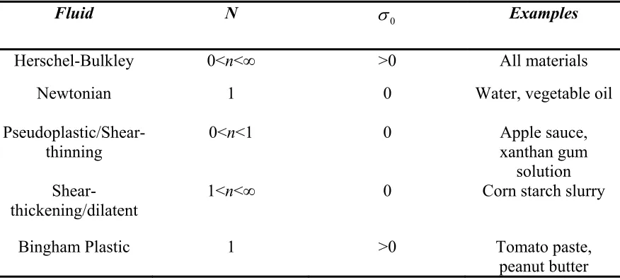
Above the yield stress, flow is induced. Table 1.1 shows common variations of fluid
rheological behavior models derived from the Herschel-Bulkley model, as compiled from
Table 1.1:
Variations of the Herschel-Bulkley Model
Fluid N σ0 Examples
Herschel-Bulkley 0<n<∞ >0 All materials
Newtonian 1 0 Water, vegetable oil
Pseudoplastic/Shear-thinning
0<n<1 0 Apple sauce,
xanthan gum solution
Shear-thickening/dilatent 1<n<∞ 0 Corn starch slurry
Bingham Plastic 1 >0 Tomato paste,
peanut butter
A shear-thinning material, also known as pseudoplastic, exhibits a decreasing viscosity as
shear rate is increased. A shear-thickening, or dilatent, material exhibits an increasing
viscosity as shear rate is increased. It is important to note that all of these models imply
that the material flow behavior is time-independent, meaning that the rheological
behavior of the fluid will not change over time.
There are also time-dependent fluids. If a fluid is mixed at a constant rate for a
given period of time and the viscosity of the fluid decreases, it is said to be thixotropic. If
the fluid increases in viscosity while mixing at a constant rate, it is said to be rheopectic.
1.2.4 Rotational Viscometry
Rotational viscometry is generally used to characterize the flow properties of a
to flow properties of a fluid material. This approach involves a cylindrical bob sitting
inside a cup, with a constant gap between the cup and bob. Instruments capable of
collecting this data usually measure two properties, angular velocity (Ω, radians/sec) and
the torque (M, Newton-meters) required sustaining the angular velocity (Steffe, 1996).
After completing these measurements, torque and angular velocity can be converted to
shear stress and shear rate, respectively, using simple calculations. The following
equation is used to determine shear stress from torque and information about the
measurement system:
2
2 hRb M
π
σ = (eq. 1.8)
where h is the height of the bob and Rb is the bob radius. The shear rate can be
determined from the angular velocity and system parameters utilizing the following
equation:
b c
b
R R
R − Ω =
γ& (eq. 1.9)
where Rc is the radius of the cup. It should be noted that this representation for shear rate
is most appropriate when Rc-Rb<<Rb, and simple shear conditions apply. Using these
calculations to solve for shear rate and stress, a constitutive equation can be determined
1.2.5 Pipeline Design Calculations
According to Steffe and Daubert (2006), pump and pipeline design in a fluid
processing system are strongly influenced by the rheological properties of a material.
Calculations that predict pressure drop and power requirements for pipeline design enable
a processor to better select manufacturing equipment.
The first step when making pipeline design calculations is to perform a
mechanical energy balance on the system. This well-known balance is expressed as:
0 ) ( ) ( )
( 2 1
1 2 2
1 2
2 + − + − +Σ + =
⎟⎟ ⎠ ⎞ ⎜⎜ ⎝ ⎛ − W F P P z z g u u ρ
α (eq. 1.10)
In this equation, the first term is a kinetic energy term, or the energy due to the fluid’s
motion. The symbols u1and u2 refer to the average volumetric velocity of the material at
two specified locations, one pre- and one post-pump position. The term αis the kinetic
energy correction term, and has the value of 2 for turbulent flow and 1 for laminar flow
(if the material is Newtonian). The second term is the potential energy term, or the energy
stored within the fluid due to elevation changes, where g is the gravitational constant and
the z1 and z2 values are elevations of the material at specified locations. Pressure changes
during pumping are the driving force for flow. However, pressure changes throughout a
system, such as during pumping and homogenization, can cause a significant amount of
mechanical energy and must be accounted for. These pressure changes come in the next
term, with P2 and P1 representing pressures at specified points, and ρ is the density of the
including fittings, expansions and contractions. Furthermore, ΣF is defined by the following equation: ⎥ ⎥ ⎦ ⎤ ⎢ ⎢ ⎣ ⎡ + Σ = Σ 2
2 2 k u2
D L fu
F f (eq. 1.11)
For the pipe section, L is the straight line pipe length, D is the internal diameter of the
pipe, u is the velocity of the fluid, and f is the Fanning friction factor. Under laminar
flow conditions, f=16/NRE, where NRE is the Reynold’s number. The second part of the
equation is for fittings such as pipe elbows. The value of kf is dependent on the type of
fitting and u is the fluid velocity through the fitting. The final term in the energy balance
(eq. 1.10), W, is the work term, which is the energy supplied by the pump. Solving for W
enables a processor to determine the pump requirements to move a material through a
defined process.
fittings pipes
1.3 Rheological Values for Shear Energy
The ability to quantitatively characterize shear input from the mechanical
components of a process is very valuable when developing process designs and
controlling quality parameters of a shear-sensitive system (Steffe and Daubert, 2006).
Examples of these parameters could include average particle size of an emulsion, air
1.3.1 Shear Work: Quantification of total shear exposure
One technique to characterize shear measures the shearing properties of different
components found in a manufacturing process. The total exposure to shear of a food
process is an important component when describing the amount of shear energy inputted
during a process. For instance, duration and magnitude of exposure to shear conditions is
important when considering the final product quality. Shear work is a term to help
describe the total shear exposure of a processing system. According to Steffe and
Daubert (2006), “shear work” refers to energy changes in a mechanical system exposed
to a shear environment, defined as such to distinguish it from energy inputs that do not
shear the product (i.e. heat). Shear work is also cumulative, meaning that all components
of a processing environment should be individually calculated for contributions to the
work term and then added together for a total shear work value for the process. Shear
work is denoted by the term and has units of Joules per kilogram. In a batch mixing
tank mode, shear work is defined as follows:
s
W
m t
Ws = Φ (eq. 1.12)
where Φ is the power supplied to the mixer, t is the mixing time, and m is the mass of the
fluid. In a continuous mixing tank system, shear work is calculated as follows
m
Ws
&
Φ
where Φ is the power supply to the mixer and is the mass flow rate of the system.
Calculations for additional pipeline components are summarized in Table 1.2.
m&
1.3.2 Shear Power Intensity
Shear power intensity is a newly proposed shear energy value that must be
considered for all system components, describing the peak shear power exposure during a
process. This shear term is defined as the product of the shear work and the mass flow
rate of the product divided by the volume of the component. Shear power intensity,
denoted by S, represents the change in power per unit volume with units of Joules per
second*m3 or Watts per m3. In a mixing tank, shear power intensity (S) is defined as
V
S = Φ (eq. 1.14)
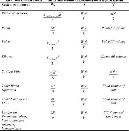
regardless of whether the operation is continuous or batch. Table 1.2 shows calculations
Table 1.2:
Shear work, shear power intensity and volume calculations for a typical system.
System component Ws S V
Pipe entrance/exit 2
/ ,
2
u kf entrance exit
V m
Ws &
2 3 D π Pump ρ P Δ V m
Ws & Pump fill volume
Valve 2
, 2
u kf valve
V m
Ws & Valve fill volume
Elbows 2
, 2
u kfelbow
V m
Ws & Elbow fill volume
Straight Pipe D u f 2 2 V m
Ws &
4 2L
D π
Tank: Batch
Operation Φmt WVsm&
Fluid volume of tank
Tank: Continuous
Flow mΦ& WVsm& Fluid volume of tank
Equipment: Pneumatic valves, heat exchangers, strainers, homogenizers ρ P Δ V m
Ws & Fill Volume of
1.3.3 Differences between Shear Work and Power Intensity
Shear work and shear power intensity vary from one another in several different
ways. One difference is that shear work is cumulative for an entire processing system
while shear power intensity only represents the power change per unit volume of any
single system component. Also, shear power intensity can be used to distinguish between
parts of a system that have identical shear work values, but have a different peak shear
exposure. For example, a long, straight length of pipe may have a shear work input
equivalent to a short pipe with several elbows. However, the shear power intensity would
show that the intensity of exposure to shear is higher in the shorter pipe that has several
elbows. Another example of the difference between shear power intensity and shear
work is described in Figure 1.2. Tank B is mixing at a much higher power setting, while
Tank A is mixing for a longer duration at a slower power setting. From the data, the
shear work (or history) of the two mixing tanks is identical. However, because Tank B is
operating with higher power or shear rate compared to Tank A, the material is sheared
with a greater intensity. Although the shear histories of the fluid inside the tanks are
Tank A
Φ= 30 Watts t = 100 sec
Tank B
Φ=300 Watts t = 10 sec Ws: Tank A = Tank B
S: Tank A > Tank B
Figure 1.2: Comparison of shear work and shear power intensity.
According to Steffe and Daubert (2006), shear work and intensity can predict the
optimal layout of a process and the type and operation parameters for a specific piece of
equipment. Predicting optimal processing design and layout may be done by establishing
critical values of shear work and shear power intensity for any given food product.
However, since all food products and processes are different, critical values for these
parameters must be independently established. Once a critical value is established,
processing conditions can be designed to stay within those critical limits. Steffe and
Daubert (2006) provide examples of product quality characteristics such as particle size
distributions of an emulsion, rheological properties of a yogurt, or the microbial colony
count of an industrial fermentation broth.
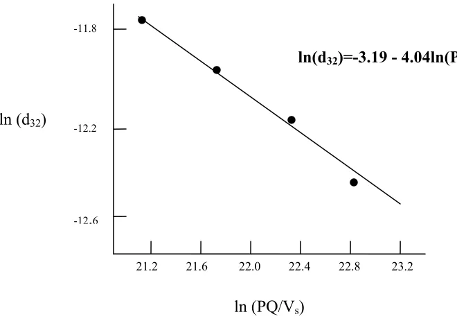
Other researchers have also attempted to predict properties of a model food
system by analyzing the power density of a process. In one such study (Tcholakova et al,
2004), the power density of energy dissipation within an emulsification chamber was
calculated to predict the mean drop diameter of a model soybean oil-in-water emulsion
conditions during emulsification play a decisive role at high emulsifier conditions.” In
this study, power density (PD) was calculated by
V PQ
PD= Δ (eq. 1.15)
where is the pressure difference in the emulsification element, Q is the flow rate, and
V is the volume of the mixing element. This term is similar to the Steffe and Daubert
(2006) calculation of shear power intensity, where the power intensity of an
emulsification element was determined by
P Δ
V m P
S =Δ &ρ (eq. 1.16)
The value of PD resulted in units of Joules/m3s as did the calculation for shear power intensity, S. The research by Tcholakova and his co-researchers found that in a
surfactant-rich emulsion, the natural log of the mean droplet size is linearly related to the
21.2 21.6 22.0 22.4 22.8 23.2
-11.8
-12.6 -12.2
ln (PQ/Vs) ln (d32)
ln(d32)=-3.19 - 4.04ln(PQ/Vs)
Figure 1.3: From Tcholakova et al, linear relationship between particle size (ln d32) and energy dissipation (ln pQ/Vs).
1.4 Emulsions
An emulsion is a heterogeneous system, consisting of at least one immiscible
liquid dispersed in another in the form of droplets, with a dispersed phase diameter
greater than 0.1 μm (Becher, 2001). Generally, there are two primary phases to an
emulsion, the dispersed and the continuous phase. The droplets are known as the
dispersed phase, while the suspending liquid is the continuous phase. In the case of an
oil-in-water emulsion, the oil is the dispersed phase while the water is the continuous
phase. For this literature review, oil-in-water emulsions will be the focus.
While the continuous and dispersed are the primary phases of an emulsion, a
emulsifier is a surface active molecule that adsorbs to the droplet surface of freshly
formed emulsions, imparting a protective membrane that prevents the dispersed phase
droplets from aggregating (McClements, 2005). During emulsification, two fundamental
processes affect the stability of an emulsion: drop rupture and coalescence. Emulsifiers
affect these processes by reducing the interfacial tension and energy, thereby promoting
rupture and providing a barrier to coalescence via interactions between adsorbed layers
on two colliding droplets (Lobo and Svereika, 2003). This phenomenon will be
discussed in depth in Section 1.7.2.
Food emulsions contain a wide range of ingredients, including flavor and color
components, preservatives, salts, sweeteners, chelating agents, and buffers. However,
three essential categories of ingredients are commonly considered the core constituents of
an oil-in-water emulsion: 1) the continuous water phase, 2) the dispersed oil phase, and
3) the emulsifier phase. The next two sections will deal with the two bulk phases,
continuous water and dispersed oil.
1.4.1 Water: Continuous Phase
Water, or a compound that has water as its primary constituent, makes up the bulk
of the continuous phase in many oil-in-water emulsions, such as milk (serum) and salad
dressing (vinegar). Water is an excellent solvent and many food emulsions contain
multiple solutes, such as colorants, salts, flavoring agents, and preservatives that are
mixed or dissolved into the water phase prior to emulsification. For instance, the aqueous
xanthan gum). The unique molecular and structural properties of water permit critical
interactions with solutes. For example, water is a very polar molecule and has the ability
to form hydrogen bonds with itself and many other polar molecules (Bryant and
McClements, 1998). Water can tightly interact with free ions, such as Na+, as well as
form hydrogen bonds (for instance, with alcohol species). However, because non-polar
molecules do not have the ability to form hydrogen bonds, a water molecule is less
attractive to non-polar molecules. When a non-polar molecule, such as oil, is introduced
to pure water, the water molecules reorient themselves to maximize the number of
hydrogen bonds formed with other water molecules, forming a “cage-like” structure also
called “hydrophobic hydration” (McClements, 2005). Properties of water related to
polarity and its ability to form hydrogen bonds account for its ability to be an excellent
solvent, as well as its inability to associate with oil or other hydrophobic molecules.
1.4.2 Oil: Dispersed Phase
Oils are part a group known as lipids, defined as being soluble in organic solvents
but insoluble in water (Potter and Hotchkiss, 1998). The most common type of lipid in
foods is triacylgylcerols, and is often the material that is commonly referred to as oil
(when liquid) or fat (when solid). Food emulsions can contain lipids that are either liquid
oil or solidified fat. For instance, milk contains a range of lipid sources that are both
Generally, lipids with shorter fatty acid chain lengths and a greater number of double
bonds have a lower melting point. These lipids that are found in foods are derived from
animal and plant tissues.
Oil plays a critical role in physicochemical, nutritional, and organoleptic
properties of emulsions. Like water, oil can be a carrier solvent for many oil-soluble
flavors, vitamins, preservatives, and other ingredients. Changing the amount of oil
present, or disturbing the structure of an emulsion, may be detrimental to both nutritional
and organoleptic properties of the food emulsion. Furthermore, the appearance of
emulsions is driven by the oil phase (Chantrapornchai et al, 1998). The characteristic
cloudiness or milky appearance is a result of light-scattering caused by oil droplets in the
dispersed phase. The greater the concentration of oil droplets, or the smaller the particle
size, the greater the degree of light scattering. The rheological properties of emulsions
are also influenced by the oil-dispersed phase. For instance, the overall viscosity of an
emulsion increases with increasing oil droplet concentration (McClements, 2005).
For emulsions, the most important part of oil is its physicochemical properties,
including oil interactions with itself and other molecules. As previously stated, an
emulsion is a mixture of two immiscible substances. Oil and water are immiscible
because of the polarity, density, and viscosity differences between the two components.
The tendency to associate via hydrophobic interactions as opposed to hydrogen bonding,
as is the case with water, is attributed to the non-polarity of oil. Hydrophobic interactions
are strong interactions between non-polar groups in the presence of water (Bryant and
water molecules, and not with non-polar oil molecules, the mixing of oil and water is
thermodynamically unstable. Because of this instability, the system minimizes the
interaction and contact area between oil and water, resulting in separation of the phases,
where the oil forms a separate layer on top of the water (McClements, 2005) as
predicated by differences among phase densities.
1.5 Emulsifiers
An emulsifier is any compound considered “surface-active,” meaning the
emulsifier molecule can adsorb to an oil-water interface and prevent emulsion droplets
from aggregating. Emulsifiers can extend the time required for an emulsion to coarsen,
or aggregate and form larger effective particle sizes, from a few minutes to a few years
(Salmon et al, 2003). Emulsifiers are amphiphilic, meaning both polar and non-polar
regions are found within the molecule. This property allows the emulsifier to interact
with both the continuous and dispersed phases, forming a membrane at this interface to
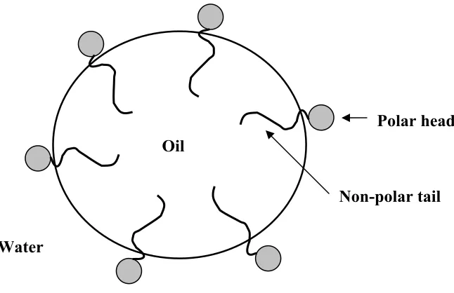
prevent dispersed phase droplets from contact. Two broad categories of emulsifiers exist:
small-molecule surfactants and amphiphilic biopolymers. A simple example of how
emulsifiers work is shown in Figure 1.4, which shows the surfactant molecule aligning so
that the non-polar tail associates with the oil phase and the polar head associates with the
Water
Polar head
Non-polar tail Oil
Figure 1.4: Emulsifier interaction at an oil/water interface.
1.5.1 Surfactants
Surfactants are small surface-active molecules that consist of a hydrophilic head
group and a lipophilic tail group. Surfactants are distinguished by the characteristics of
either the hydrophilic or lipophilic groups. The head group is classified as anionic
(negatively charged surfactant), cationic (positively charged), nonionic (non-charged), or
zwitterionic (overall charge of 0, but carries positive and negative charges). The tail
group is characterized by the length of the hydrocarbon chain, the degree of branching,
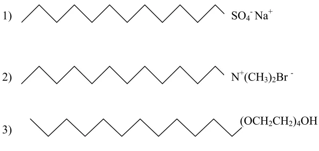
and the degree of saturation. Several surfactants are displayed in Figure 1.5. Surfactants
can be soluble in either water or oil. Bancroft’s rule states that the phase in which a
(OCH2CH2)4OH 2)
SO4-Na+ 1)
N+(CH3)2Br
-3)
Figure 1.5: Drawing of surfactant structures: I-anionic (sodium dodecyl sulfate); 2-cationic (dodecyltrimethylammonium bromide); and 3-non-ionic [n-dodecyl tetra (ethylene oxide)]; Source: Rangel-Yangui et al, 2005
The Hydrophile-Lipophile Balance (HLB) is the classification system describing
the degree to which a surfactant is soluble in either water or oil. The HLB values were
originally determined in 1949 by Griffin (Govin and Leeder, 1971), and the following
formula was developed for polyoxyethylene derivatives of fatty alcohols and polyhydric
alcohol fatty acid esters (Becher, 2001):
HLB= 20 ⎟
⎠ ⎞ ⎜ ⎝ ⎛ −
A S
1 (eq. 1.17)
where S is milligrams of NaOH required to saponify 1 gram of the ester and A is the
milligrams of NaOH required to neutralize the acid part. In another widely used method,
Davies (Guo et al, 2006) developed the following equation to calculate HLB values (Guo
HLB = 7 + Σ(hydrophilic group numbers) – Σ(lipophilic group numbers) (eq. 1.18)
where the hydrophilic and lipophilic group numbers correspond to the type of hydrophilic
or lipophilic group(s) attached to the surfactant. Although this method is relatively easy
to use, it is not applicable to all surfactants, and experimentally determined HLB values
are sometimes far from the value calculated using the Davie method (Guo et al, 2006).
Much research has been done to improve the HLB calculation, including accounting for
fatty acid chain length and critical micelle concentration (Lin et al, 1973), which is the
concentration at which surfactant molecules form micelles with each other. The HLB
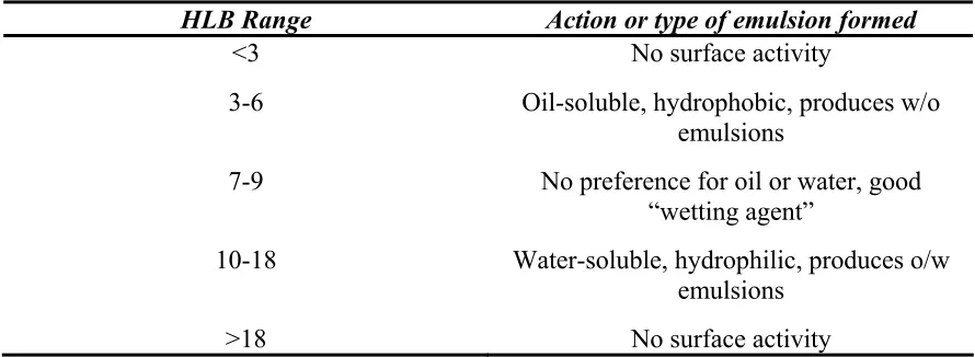
values of common surfactants are shown in Table 1.3. An HLB value between 3 and 6
signifies highly hydrophobic surfactants, oil soluble, and will produce stable water-in-oil
(continuous phase is oil) emulsions. An HLB value between 10 and 18 represents a
hydrophilic surfactant that will form clear solutions with water and stabilize O/W
emulsions. Intermediate HLB values (7-9) indicate no preference for either oil or water,
and are considered good “wetting agents” (McClements, 2005). An extremely low (less
than 3) or high (over 18) HLB value indicates the molecule is not surface active and will
not accumulate at interfaces. The HLB system is useful for choosing the optimal type of
emulsifier for an emulsion system and is of practical use for both single emulsifiers and
mixtures of emulsifiers (Velev et al, 1994). Table 1.4 summarizes the surfactant action in
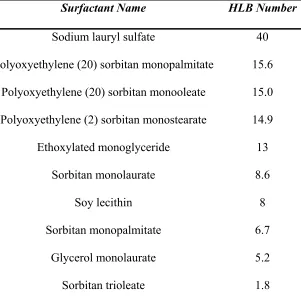
Table 1.3:
Common surfactants and their associated HLB values.
Surfactant Name HLB Number
Sodium lauryl sulfate 40
Polyoxyethylene (20) sorbitan monopalmitate 15.6
Polyoxyethylene (20) sorbitan monooleate 15.0
Polyoxyethylene (2) sorbitan monostearate 14.9
Ethoxylated monoglyceride 13
Sorbitan monolaurate 8.6
Soy lecithin 8
Sorbitan monopalmitate 6.7
Glycerol monolaurate 5.2
Sorbitan trioleate 1.8
Table 1.4:
The action and type of emulsion formed at various HLB values.
HLB Range Action or type of emulsion formed
<3 No surface activity
3-6 Oil-soluble, hydrophobic, produces w/o emulsions
7-9 No preference for oil or water, good “wetting agent”
10-18 Water-soluble, hydrophilic, produces o/w emulsions
>18 No surface activity
1.5.1.1 Critical Micelle Concentration
Critical micelle concentration (CMC) is another important aspect of emulsions.
The CMC is the critical level of surfactant where the molecules begin to form micelles
with one another (Dickinson, 1992). Below this level, the surfactant predominantly acts
as a monomer, while above this concentration the surfactant begins to associate with
itself. The surface tension of an emulsion decreases as surfactant is added below the
CMC, making the emulsion more stable. However, once this value is exceeded, the
surface tension is consistent because surfactant micelles are coated on the outside with
their hydrophilic head, and thus have little surface activity compared with surfactant
monomers.
1.5.1.2 Cloud point
The cloud point of an emulsion is the point where the solution becomes turbid,
micelles become aggregated because of dehydration of polar head groups at higher
temperatures, altering the molecular geometry and decreasing repulsion between the
surfactant molecules (McClements, 2005). At elevated temperatures, the aggregates can
become significant enough to sediment under gravity, forming a separate phase that can
be visually observed.
The cloud point is an important consideration with any thermal process. If the
cloud point is breached, the surfactants ability to stabilize an emulsion is greatly
diminished. However, at temperatures immediately below the cloud point, oil drop
rupture is greatly increased because of decreased interfacial tension between oil and
water, permitting smaller droplet sizes with the same energy input.
1.5.2 Tween-series surfactants
“Tween” or “Polysorbate” is the trade name given to polyoxyethylene sorbitan
esters that are hydrophilic surfactants. Tween surfactants are used to make very stable
O/W emulsions and are extremely soluble in water. Produced by reacting esterified
polyols with fatty acids, Tweens are classified according to the type of fatty acid that
reacts with ethylene oxide, for instance Tween 20 (polyoxyethylene sorbitan
monolaurate) and Tween 80 (polyoxyethylene sorbitan monooleate) (Yeh et al, 1999).
Tween-series surfactants are used in a variety of food, pharmaceutical, and other
applications. In the food industry, Tweens are used for stabilization of salad dressings
and as a wetting agent for many products such as candies, where it is used to enhance
Figure 1.6: Structure of Tween 20; Source: Balakrishnan et al, 2005
Tweens are known for high HLB numbers, suitable as surfactants for oil-in-water
emulsions. A table of properties of Tween-series surfactants is shown as Table 1.5. The
table shows the full chemical name of the surfactant, molecular weight, HLB value, and
critical micelle concentration. Compared to whey or casein proteins, which have a
molecular weight in the range of 20,000, the Tween surfactants are small. Figure 1.6
Table 1.5: Properties of Tween series surfactants
Surfactant Name Molecular
Weight
HLB CMC (mM)
Tween 20:
polyoxyethylene (20) sorbitan monolaurate
1227.54 16.7 0.05
Tween 60:
polyoxyethylene (20) sorbitan monostearate
1311.70 14.9 0.021
Tween 80:
polyoxyethylene (20) sorbitan monooleate
1309.68 15.0 0.01
Source: From Table 1 in Hsu and Nacu, 2003
1.6 Emulsion Formation
Emulsions are formed by applying sufficient mechanical energy to disperse one phase of
the emulsion into the other phase (Narsimhan and Goel, 2001). The amount of
mechanical energy required to form an emulsion is related to the free energy of emulsion
formation (ΔGformation). The amount of free energy required to increase the area of an
oil-water interface (i.e. reduce the droplet size) is given by the following relationship:
A I
G= tΔ
Δ (eq. 1.19)
where It is the interfacial tension and ΔA is the increase in oil-water interface area caused
by a decrease in droplet size (Dickinson, 1992). However, the actual amount of
be the Laplace pressure. The Laplace pressure is the interfacial force responsible for
keeping a droplet in a spherical shape, defined as
ΔPL= 4It/d (eq. 1.20)
where It is interfacial tension and d is droplet diameter. Therefore, to disrupt a droplet of
radius a, the following pressure gradient (
dr dP
) must be applied (Dickinson, 1992):
2 2 ~
a I a P dr
dP L t
= Δ
(eq. 1.21)
To deform or disrupt a droplet, it is necessary to apply mechanical energy that is
significantly larger than the pressure gradient and the Laplace pressure. Equations
1.19-1.21 indicate that the amount of force required to disrupt a droplet increases as surface
tension is increased or as droplet diameter is decreased. During emulsification, oil
droplets collide and coalesce with one another and form larger droplets, which will
accelerate the creaming process and prompt the emulsion to revert back to a more
thermodynamically stable form (i.e. two separate states, oil and water). Therefore, an
emulsifier must be added to adsorb to the oil droplet surface and provide a protective
membrane preventing other oil droplets from approaching and coalescing. According to
McClements, the size of droplets produced during homogenization depends on two
processes: the initial generation of droplets of small size by the input of mechanical
energy, and the rapid stabilization of the droplets against coalescence following
The mechanical energy required to form small droplets can be applied in a variety
of ways and can be as simple as shaking or stirring the two immiscible phases together.
However, more complicated mechanical devices are usually used to form emulsions. The
name given to converting two immiscible liquids into a more stable emulsion is known as
homogenization. There are many different categories and types of homogenizers that
form emulsions in different ways. Homogenizers and the mechanical principles behind
homogenization are discussed in the following sections.
1.6.1 Homogenization
Homogenization as a specific unit operation has existed since 1900, when Auguste
Gaulin invented and presented the first homogenizer invention at the World Fair in Paris
(Paquin, 1999). According to Walstra, three reasons exist for the application of
homogenization to a food product (Walstra, 1999).
1. Counteracting segregation, such as creaming, of components of the emulsion by particle size reduction;
2. Increasing stability towards coalescence by reducing particle size; and
3. Creating desirable rheological properties. For instance, a decrease in fat particle size in milk increases the viscosity of a fluid milk or cream.
All of these reasons are achieved by decreasing the fat droplet size within the dispersed
phase. Homogenization is generally divided into two categories, primary and secondary.
Primary homogenization is comprised of the mixing of two completely separate,
emulsion generally contains large particle sizes and is usually only maintained for a short
period of time (compared to secondary homogenization). An example of a product made
from primary homogenization is home-made salad dressing, where a quantity of oil and
water-based ingredients are mixed together from separate phases, either by hand or with a
small blender. It is important to note that a traditional high-pressure homogenizer, such
as one used by a dairy plant, cannot be used for primary homogenization and is only used
for particle size reduction. Secondary homogenization is the reduction of particle size in
an already pre-existing coarse emulsion. Since secondary homogenization produces
smaller particle sizes, the resulting emulsion is stable for a much longer period of time
than a coarse emulsion. Homogenization in dairy processing, for example, reduces fat
globules in raw milk to below 1 μm in size. Un-homogenized milk will usually form a
visible cream layer within 1-2 days, while homogenized milk will remain stable and
exhibit no visible creaming for several weeks.
When immiscible substances are forced through a narrow opening (Walstra,
1999), called the homogenizer valve, homogenization occurs. The high pressures
generate a tremendous amount of energy and fluid velocity, resulting in intense
turbulence. Bernoulli’s equation, shown as equation 1.22, governs the conversion of
energy to disrupt fat droplets.
2 2 2
2 1
1 2
1 2
1
u P
u
P + ρ = + ρ (eq. 1.22)
where the left side of the equation represents the system prior to homogenization and the
simplification, P1 is the homogenization pressure (Phom), P2is 0 (since it is open to the
atmosphere), and the ρ and u terms are the densities and velocities of the product pre-
and post-homogenization. In the case of homogenization, u1<<u2, therefore
2 2 hom
2 1
u
P = ρ (eq. 1.23)
where Phom is the homogenization pressure and ρ and v are the density and velocity of the
fluid, respectively. Thus, the fluid velocity in the homogenization valve can be
calculated, and from this value the energy dissipation, or power density, caused by
homogenization can be discerned. Energy dissipation, with units of W/m3 is given by
p DISS
t P
E = hom (eq. 1.24)
where tp is the passage time of the fluid being homogenized, found by dividing the length
of the homogenization valve by u2. In the case of homogenizers, EDISS can be very
intense, often in the range of 1011-1012 W/m3. While greater than 90% of this energy is converted to heat, the remaining energy produces intense turbulence, causing eddies to
form within the homogenizing liquid. The eddies, in turn, cause pressure fluctuations
that disrupt fat droplets or particles, causing a reduction in globule size (Walstra, 1999).
1.6.1.1 Droplet Disruption
Fat droplet disruption is determined by the balance between interfacial forces and
disruptive forces. As stated previously, the Laplace pressure is the force responsible for
forces is of sufficient duration, a fat droplet will be broken up. The Weber number is a
dimensionless term that defines the ratio between disruptive (or shear) and interfacial
force.
We=shear forces/interfacial forces=
t c I d 2 η γ& (eq. 1.25)
whereγ& is the shear rate, ηc is the viscosity of the continuous phase, d is the diameter of
the droplet, and It is the interfacial tension. This equation is used during simple shear
flow (McClements, 2005). The disruptive forces, however, are often very difficult to
calculate due to the complex nature of a flow regime within an emulsion. By assuming a
flow regime to be either turbulent or laminar, the maximum size of droplets remaining
following homogenization can be predicted. Under laminar flow conditions, the
following equation applies:
c cr tWe I d η γ& 2
max = (eq. 1.26)
where Wecris the critical Weber number required to produce droplet deformation, It is
surface tension, γ& is shear rate, andηc is the viscosity of the continuous phase. Wecr is
dependent upon the ratio between continuous phase viscosity and dispersed phase
viscosity, with ratios between 0.1 and 1, resulting in a minimum value of Wecr. Under
turbulent conditions, the following equation predicts maximum size of fat droplets, dmax
c t E I d η =
where E is the power density created by emulsification (eq. 1.24), and all other variables
are similar to the previous laminar flow condition equation. It should be noted that since
homogenization is a very complex and dynamic process, homogenization is actually a
combination of both laminar and turbulent flow conditions in undefined amounts.
However, the above calculations can be used by food processors to determine the
required energy or shear rate input needed to produce an emulsion of a specified droplet
size.
1.6.1.2 Droplet Coalescence
Fat droplets in emulsions, during or after homogenization, are constantly moving
due to gravity, Brownian motion, or the mechanical action of homogenization
(McClements, 2005). Because of this motion, droplets frequently collide and have a
tendency to coalesce providing there is an insufficient amount of emulsifier present to
stabilize the system. As stated by Narsimihan and Goel (2001), “if the timescale of
collision is smaller than the timescale of absorption, the fresh interface of a newly formed
droplet will not be fully covered with surfactant before it’s encounter with another
droplet.” The degree of coalescence and the fat droplet sizes produced during
homogenization is a ratio of the time taken for the emulsifier to adsorb to the surface of
the droplets (τADS) and the time between droplet collisions (τCOL) (McClements, 2005).
To produce an emulsion with a small droplet size, a ratio ofτADS / τCOL is ideally required
to be much less than 1 (McClements, 2005). The following equation has been given to
c COL
ADS
dm
φ π τ
τ ≈6 Γ
(eq. 1.28)
where Γ is the excess surface concentration of surfactant, mcis the emulsifier
concentration, d is the droplet diameter, and φ is the dispersed phase volume fraction. A
study by Narsimhan and Goel on a tetradecane-in-water emulsion stabilized with sodium
dodecyl sulfate showed a relationship similar to equation 1.28. Coalescence rate
constants were higher with smaller drop sizes and lower emulsifier concentration, but the
rates were notably higher at elevated pressure settings (Narsimhan and Goel, 2001). This
result demonstrates that as homogenization pressure or total energy input is increased, the
rate of coalescence will increase. Similarly, Taisne et al (1996) showed that
re-coalescence occurring in previously homogenized emulsions developed when
homogenization pressure was increased above the original homogenization pressure.
Furthermore, in a study by Lobo and Svereika (2003), increasing the fraction of oil phase
increased the coalescence rate by increasing the frequency of droplet collision. The rate
of coalescence has many deciding factors, and these factors must be considered when
determining the degree to which coalescence impacts an emulsion.
1.7 Emulsion Stability/Instability
Emulsion stability is a relative term to describe the degree to which changes occur
to the emulsion quality with time (McClements, 2005). Some emulsions, such as bottled
salad dressings or mayonnaise, are required to remain stable for several months or even
several minutes or hours. From a thermodynamic standpoint, emulsions are almost
always unstable due to the increase in interfacial area after emulsification, leading to an
increase in free energy. In an emulsion, the free energy of emulsion formation (or
ΔGformation) is equal to the interfacial tension (It) at the oil-water interface multiplied by
the increase in surface area created during emulsification, or,
ΔGformation= ItΔA (McClements, 2005) (eq. 1.29)
Given time, all emulsions will eventually break down (meaning a decrease in surface
area, ΔA) and are considered to be kinetically stable or metastable. Upon emulsification,
the total free energy is increased because of an increase in ΔA. Driven by
thermodynamics, the system attempts to reduce the amount of free energy by decreasing
ΔA (i.e. phase separation). However, an emulsion may have metastable states where an
increase in free energy, called free energy barrier or activation energy, is required to
move to a more thermodynamically stable state. If these free energy barriers are large
enough, an emulsion may remain metastable for a very long time. Examples of free
energy barriers are surfactants or emulsifiers that prevent dispersed phase droplets from
coming in contact.
The instability of emulsions can take several forms. Dickinson (1992) listed five
primary instability modes: 1) Creaming and Sedimentation, 2) Phase Inversion, 3)
Ostwald ripening, 4) Flocculation, and 5) Coalescence. The creaming rate of an emulsion
is the most important of these instability modes, and is often influenced by each of the
four other forms of instability. However, each of these forms manifests itself differently,
1.7.1 Creaming and Sedimentation
Creaming or sedimentation involves the gravitational separation of the dispersed
phase from the continuous phase, earning its name from the separation of cream from
un-homogenized milk. The process is referred to as creaming when the droplet phase is less
dense than the continuous phase, and thus the droplets rise upward, as is the tendency for
oil-in-water emulsions. The process is referred to as sedimentation when the droplet
phase is denser than the continuous phase, and will move downward, as is the tendency
of water-in-oil emulsions.
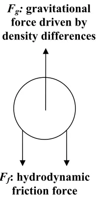
The rate of creaming is described by Stoke’s Law, which includes a combination
of gravitational and hydrodynamic friction forces that acting in opposite directions to
retard droplet motion as is shown in Figure 1.7 (McClements, 2005). The upward
gravitational force (Fg) is described with the following force balance,
g r
Fg ( )
3 4
1 2 3 ρ ρ
π −
−
= (eq. 1.30)
where r is the droplet radius, g is the acceleration due to gravity, and ρ is the density,
with subscripts 1 and 2 referring to the continuous and dispersed droplet phase,
respectively. The negative sign in equation 1.30 is attributed to the lower density oil
phase being force upward by the buoyancy force associated with the continuous phase.
The gravitational force is upward because the oil droplet will rise with it having a lower
density. The hydrodynamic friction force is given by
rv
where v is the creaming velocity and η1 is the shear viscosity of the continuous phase.
Fg: gravitational
force driven by density differences
Ff: hydrodynamic
friction force
Figure 1.7: Description of Fg and Ff forces that drive stokes law
The particle will reach a constant velocity, when Fg=Ff, and thus the Stoke’s Law
equation is derived,
1 1 2 2
9
) (
2
η ρ
ρ −
−
= gr
vStokes (eq. 1.32)
This equation is useful for predicting creaming time for a simple emulsion. Furthermore,
eq. 1.32 also displays useful information about managing emulsion separation. The
creaming velocity of an emulsion can be slowed by a number of strategies, evidenced by
droplet
rtant
ase,
eristics of an emulsion
system edian particle size, viscosity and dispersed phase volume can be useful
rage creaming rate using Stokes Law.
.
their
esce. Therefore, coalescence can be inhibited by a) smaller size, or reducing the density difference between the continuous and dispersed
phase will slow the creaming rate and improve emulsion stability.
Stokes Law, however, is simplistic and does not consider a number of impo
features, including polydispersity, droplet flocculation, concentration of dispersed ph
non-Newtonian rheology of continuous phase, droplet fluidity, fat crystallization,
electrical charge, Brownian motion, and adsorbed layer characteristics. When these
effects are combined, the ability to accurately model creaming behavior of an emulsion is
more complex. However, knowledge of some basic charact
, such as m
in estimating the ave
1.7.2 Coalescence
Coalescence is the process by which two or more dispersed droplets come in
contact and merge together forming a single larger droplet, as illustrated in Figure 1.8
Coalescence causes droplets to cream or sediment more rapidly due to an increase in
effective size that occurs when the material separating the two droplets is disrupted.
Droplet rupture is more prone to occur as two droplets come closer together. Upon
approach, the interface between two droplets becomes flattened. The tendency for
droplets to become deformed is described by the Weber number, which was described in
section 1.6.1.1. At lower levels of the Weber number (We<1), the droplets tend to remain
spherical, resisting coalescence. At Weber numbers above 1, the droplets are more likely
droplet radius, b) lower external force, c) higher surface tension, and d) higher separation
distance between droplets.
Figure 1.8: Depiction of coalescence: 1) Droplets approach and collide with each other, 2) Collision force is great enough to disrupt membrane, or there is insufficient emulsifier coverage and the droplets stick to one another,
larger droplet.
s will 1
2
3
3) Coalescence occurs, with two smaller droplets becoming one
In most food emulsions, film disruption occurs from either insufficient
emulsifier, film stretching, or the film tearing. If there is insufficient emulsifier, gaps at
the interface will exist, and coalescence will occur if two gaps contact one another.