ABSTRACT
KULKARNI, VINEET ASHOK. Social Distance Aware Resource Allocation. (Under the direction of Michael Devetsikiotis.)
Communication flows associated with human end-users will have an underlying social
con-text which determines the importance of the communication. In other words, the network gives us the capability to communicate, but the reason to communicate is external to it. In order
to facilitate communication flows, the network has to make decisions on resource allocation
to the flows among several others (admission control, traffic policing and so on). If the net-work remains agnostic to the underlying social context of the communication flow, the resulting
decisions will at best be sub-optimal when viewed along the social context dimension.
In this work, we measure the social context associated with a communication flow and incorporate it into resource allocation decisions at the network. We use the notion of social
distance between end-users to measure corresponding context. We combine the social distance
as declared by the end-user with the overall importance of the user in the social network to derive a social-network-wide social distance measure. Further, we define social distance aware
utility functions by imposing maximum achievable utility bounds on the communication flows
based on the social distance. This ensures that in an optimal allocation of resources, flows of the same traffic type get differentiated service based on the associated social distance.
We present the resultant resource allocations with respect to wireless networks. Specifically,
we look at the case of voice flows competing for resources over an IEEE 802.11e QBSS, and provide theoretical as well as simulation results demonstrating that our social distance aware
resource allocation (SDA) achieves higher network utility than IEEE 802.11e for every case considered. We also look at the case of both voice and video calls competing for resources and
show that SDA achieves improved network utility as compared to IEEE 802.11e. The reason
for this is that SDA allocates resources based on classifying flows through the social distance dimension, as compared to IEEE 802.11e which only takes into account the traffic type for
classification.
When users are requesting content hosted on the network, the relationships between con-tent can be used to determine relative importance of concon-tent. In the case of social concon-tent
(Youtube), such relationships are well-defined and thus the social network is already
deter-mined. After defining a corresponding social distance measure for videos, we look at three centrality techniques (degree, closeness, betweenness) to determine which of the three performs
optimally in determining the most accessed videos. Finally, we look at some of the applications
©Copyright 2012 by Vineet Ashok Kulkarni
Social Distance Aware Resource Allocation
by
Vineet Ashok Kulkarni
A dissertation submitted to the Graduate Faculty of North Carolina State University
in partial fulfillment of the requirements for the Degree of
Doctor of Philosophy
Computer Engineering
Raleigh, North Carolina
2012
APPROVED BY:
Mihail Sichitiu Wenye Wang
Rudra Dutta Michael Devetsikiotis
DEDICATION
BIOGRAPHY
The author completed his B.E. at SDM, Dharwad in the year 2002. After working for 2 years,
ACKNOWLEDGEMENTS
I would like to thank my Advisor, Prof. Michael Devetsikiotis for his help in all my work. I am
especially grateful for the freedom that he gave us (all of his students) in pursuing out ideas and working on them. I am also grateful to Prof. Mihail Sichitiu for his help and guidance during
my PhD. I learnt a lot working on the mesh network project about the hardware of wireless
networking for which I am grateful. I want to thank Prof. Wenye Wang and Prof. Rudra Dutta for their encouragement and direction in my work.
I would like to thank Prof. Sichitiu and Prof. Viniotis for trusting me with ECE 470. This
course made my life at NC State more enjoyable than almost anything else. I would also like to thank Marhn Fullmer for helping me out of hardware issues innumerable times.
TABLE OF CONTENTS
List of Tables . . . vii
List of Figures . . . .viii
Chapter 1 Introduction . . . 1
1.1 Motivation . . . 1
1.2 Objectives of Resource Allocation . . . 3
1.2.1 Flow Allocation and Traffic Matrices . . . 3
1.2.2 Routing and Resource Management . . . 4
1.2.3 Performance Measurement and Network Control . . . 5
1.2.4 Resource Allocation . . . 6
1.2.5 Predicting Traffic Matrix . . . 7
1.3 Implications of Social Context . . . 7
1.3.1 Predicting Traffic Intensity . . . 7
1.3.2 Deriving Social Graphs . . . 8
1.3.3 Other Applications . . . 8
1.4 Scope and Objectives . . . 8
1.4.1 Objectives . . . 9
1.5 Overview of Thesis . . . 10
Chapter 2 Social Networks and Social Distance . . . 12
2.1 Motivation . . . 13
2.2 Social Distance . . . 14
2.2.1 Centrality and Social Distance . . . 15
2.3 Utility Optimization . . . 16
2.3.1 The functionf . . . 20
2.4 Social Distance in Content . . . 21
2.4.1 Rank Distribution . . . 21
2.4.2 Content Caching and Distribution . . . 22
2.5 Summary . . . 22
Chapter 3 Voice Call Capacity Analysis. . . 24
3.1 Background . . . 25
3.2 Simulation Setup . . . 25
3.3 Call Capacity Models . . . 26
3.3.1 Single Hop Wireless Network . . . 27
3.3.2 Two Hop Wireless Network . . . 27
3.3.3 Three Hop Wireless Network . . . 28
3.4 Sensitivity Analysis of the Call Capacity . . . 30
Chapter 4 Resource Allocation for Voice Calls . . . 31
4.1 Overview . . . 31
4.2 IEEE 802.11e QBSS and SDA Theoretical Analysis . . . 32
4.2.1 Utility Maximization . . . 33
4.2.2 Comparing IEEE 802.11e and SDA . . . 36
4.3 IEEE 802.11e and SDA Simulation . . . 39
4.3.1 Simulation Setup . . . 39
4.3.2 Utility in terms of AIFS . . . 40
4.3.3 Social Graph . . . 42
4.3.4 Comparing IEEE 802.11e and SDA . . . 43
4.4 Summary . . . 43
Chapter 5 Resource Allocation for Voice and Video Flows . . . 44
5.1 Using Social Distance for Voice and Video Traffic . . . 44
5.1.1 Simulation Setup . . . 45
5.1.2 Voice and Video Traffic Performance . . . 47
5.1.3 Discussion of Detailed Results . . . 49
5.1.4 Resource Allocation Patterns . . . 50
5.2 Social Distance and Fairness . . . 51
5.3 Summary . . . 52
Chapter 6 Social Distance Aware Content Distribution. . . 53
6.1 Motivation . . . 54
6.2 Data Collection . . . 55
6.3 Timescales . . . 56
6.4 Centrality . . . 57
6.4.1 Degree Centrality . . . 58
6.4.2 Closeness Centrality . . . 58
6.4.3 Betweenness Centrality . . . 59
6.5 Performance Analysis . . . 59
6.5.1 Standard Feeds . . . 60
6.5.2 Science and Technology Category Trace . . . 61
6.5.3 Number of videos served . . . 61
6.6 Proposed L2 Distributed Content Cache . . . 62
6.7 Summary . . . 63
Chapter 7 Experimental Data Trace Collection for SDA . . . 64
7.1 WiFi Localization . . . 64
7.1.1 Generation of the wireless map . . . 65
7.1.2 Localization of a user . . . 66
7.2 Client Applications . . . 67
Chapter 8 Conclusion . . . 69
LIST OF TABLES
Table 4.1 Network performance comparison for IEEE 802.11e vs SDA when voice calls are competing with best-effort traffic. . . 38 Table 4.2 VoIP traffic R-value, MOS, and distance modified MOS . . . 39
LIST OF FIGURES
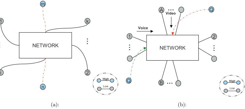
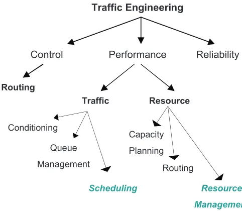
Figure 1.1 Current service differentiation schemes cannot classify voice (or video) flows into further priority classes. In Figure 1.1a, a high priority voice call is blocked due to aggressive low priority voice calls. In Figure 1.1b, a high priority video flow is blocked, when in the same scenario, a high priority voice call would have been admitted. . . 2 Figure 1.2 The scope of our work within the broader area of Traffic Engineering. . . 4 Figure 1.3 Routing algorithms compute shortest paths based on link costs. Flow
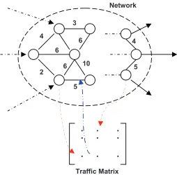
allocation depends on shortest paths to determine the optimal path and egress router for each flow. The traffic matrix depends on the flow allo-cation, and changes the link cost thereby requiring routing updates. . . . 5 Figure 1.4 The scope of our work within the broader area of Traffic Engineering. . . 9
Figure 2.1 An example organizational social network. Each user identifies his/her peers and the perceived priority of the corresponding relationship to him/her personally. . . 13 Figure 2.2 Prioritized resource allocation among three flows of the same traffic type. 19 Figure 2.3 Rank distributions for two categories of Youtube videos. . . 22
Figure 3.1 The simple chain topology used for our simulations. . . 25 Figure 3.2 System Response for 2 Hops (Figure 3.2a) and 3 Hops (Figure 3.2b) are
shown. For both cases, one of the links is set to have the data rate of 11Mbps, while the other data rates are varied. . . 28 Figure 3.3 Partial derivatives of the call capacity (for 3 hops) with respect to the
packetization interval. . . 29
Figure 4.1 The network is made aware of the social distance dependent utility, due to which it can allocate resources differently to flows of the same traffic type. Resource allocation is achieved by setting parameters on the client stations as well as the AP in the case of a wireless network. . . 32 Figure 4.2 Comparison of the total network utility achieved for IEEE 802.11e vs
So-cial Distance Aware Resource Allocation (SDA). SDA outperforms IEEE 802.11e for every case. . . 36 Figure 4.3 Maximum Call Capacity, 802.11e vs Distance-aware. 802.11e VoIP call
Figure 5.1 The network topology used for simulation is shown in 5.1a. Nodes are placed around a circle of radius 100m with the AP at the centre. Trans-mission range of all the nodes is set to 250m. 5.1b shows the modification of IEEE 802.11e AC’s to include social distance aware traffic AC’s. The corresponding AC parameters are also listed. . . 46 Figure 5.2 Network Performance for a mix of voice and video calls competing for
the shared channel. Results for NV=NVI, NV=2NVI and 2NV=NVI are shown in Figure 5.2a,Figure 5.2b,Figure 5.3a respectively. SDA performs better during saturation traffic conditions as compared to IEEE 802.11e. . 48 Figure 5.3 Specific resource allocation patterns for 5.3a are shown in 5.3b for IEEE
802.11e, and in 5.3c for SDA. White cells represent resources were allo-cated, black cells represent no resources were alloallo-cated, and grey cells represent no resources were requested. It can be seen that IEEE 802.11e allocates all requested resources to voice while starving video flows be-yond 8 flows. SDA allocates resources to both voice and video flows inχ1 before allocating resources to voice and video flows inχ2 and so on. . . . 50
Figure 6.1 Structurally Figure 6.1b has more impact on design and performance de-cisions than Figure 6.1a, but both have the same ex-or counts. Variations in the inter-relationships are plotted against time for Top Rated (Fig-ure 6.1c), Most Viewed (Fig(Fig-ure 6.1d) and Most Recent (Fig(Fig-ure 6.1e) videos. 56 Figure 6.2 Comparison of the three centrality methods for the Top Rated videos
feed. Betweenness centrality saturates earlier than the other two, it also performs poorly at choosing the best videos as compared to closeness centrality. Also, at small content cache sizes, closeness centrality performs exceptionally well than the other two. . . 59 Figure 6.3 Figure 6.3a shows the number of hits for cached videos ranked by closeness
centrality. Each cell (square) represents 16 videos, with the lower-left cell representing the most viewed and the upper-right representing the least viewed videos. Figure 6.3b shows that betweenness centrality performs poorly in choosing the right videos, since the number of hits is low across the board. . . 61 Figure 6.4 The performance of cache for Science and Technology trace is shown in
Figure 6.4a. Figure 6.4b shows a proposed L2 distributed content cache. . 62
Figure 7.1 Creating a wireless signal map of the building requires capturing RSSI information at different locations in the building. . . 65 Figure 7.2 Sequence of messages exchanged to achieve the desired objective as
Chapter 1
Introduction
Communication flows over the network are initiated by human end-users for broadly one of two reasons: the need to communicate with another end-user through a real-time communication, or
the need to view content hosted on the network which then necessitates transfer of content. The
objective of the network is to achieve the desired level of service (QoS) for end-users through the available resources. The service differentiation among such competing flows is dependent on
the media of communication (voice, video, text) and also on the importance of the flow to the
end-users themselves. Not all voice flows competing for resources are equally important, and a service differentiation scheme which prioritizes flows solely based on traffic type will result in
a sub-optimal allocation of resources. We look at the broader traffic engineering problem, and
the role of resource allocation within this in determining network performance.
1.1
Motivation
Resource allocation algorithms have been traditionally designed to optimally allocate available resources among the competing flows while satisfying certain capacity and routing constraints
imposed by the design of the computer network. In doing this, the algorithms are agnostic to
the underlying real-world social context associated with the flow that is requesting resources. This is in agreement with a core philosophy of the Internet - that of preserving anonymity of
flows. In order to accommodate inelastic flows, a degree of service differentiation is eventually
enforced through classification of the flows based on traffic type. Since different inelastic traffic types (voice, video streams) have differing expectations of the QoS (defined in terms of delay,
packet loss ratio, data rate), such a classification makes sense.
Networks have finite resources, and the allocation of these resources is FCFS (First Come First Serve), unless the network has the capability to pre-empt flows. We do not consider
NETWORK
1 k
i 2
m
n
High
Low
.. . ..
.
(a):
NETWORK
1 2
A
B High
Low
Q
Q
…
… ..
. ...
Voice
Video
(b):
Figure 1.1: Current service differentiation schemes cannot classify voice (or video) flows into further priority classes. In Figure 1.1a, a high priority voice call is blocked due to aggressive low priority voice calls. In Figure 1.1b, a high priority video flow is blocked, when in the same scenario, a high priority voice call would have been admitted.
been accepted. Service differentiation schemes help prioritize resources between accepted flows,
differentiating based on the traffic type (inelastic/elastic, voice/video). Service differentiation
alone can only provide graded service to the accepted flows. It cannot provide guarantees on the achieved QoS of a given inelastic flow because no resources are reserved beforehand.
Call admission control schemes can be used to ensure that all accepted flows are allocated the
minimum necessary resources, and none of the accepted flows are dropped due to scarcity. In such a scenario, once the capacity of the network is attained, no more flows can be
admitted until at least one flow leaves the system. This means that the instance in time at
which a flow requests resources determines whether it is admitted into the network or not. More specifically, the network state at the time instant of the incoming resource request determines
the outcome. Since the network is agnostic to the underlying social context of the flows, a high
priority flow may be denied access when low priority flows are using the network (shown in Figure 1.1). Note that the low priority flows may also all be inelastic (e.g., voice) flows. When
all the flows competing for resources belong to the same traffic type, e.g., voice (Figure 1.1a)
a high priority voice call may get blocked due to low priority calls which are aggressive in requesting resources. The request rate (for resources) determines allocation rather than the
perceived priority. Thus, knowledge of the social context can help identify the high priority flows
assuming that elastic flows do not have any minimum quality requirement from the network,
and use up whatever available resources there are. When there is an explicit priority for one type of inelastic traffic over another (voice is higher priority than video), voice calls can
effectively starve video flows out of resources as shown in Figure 1.1b. Since the video flows
have a minimum quality requirement, the flows begin to fail. When viewed along the social context dimension, the voice flows may actually be lower priority than the video flow requesting
resources. A service differentiation scheme which prioritizes flows solely based on the traffic
type cannot serve the high priority video flow at the expense of low priority voice calls. The implicit prioritization in these schemes is that voice traffic is always more important than video.
Again, social context can be used in such a scenario to elicit the real-world priority of flows to
provide improved service differentiation.
In situations where network resources are scarce, anonymity of flows (no knowledge of the
social context) can in fact result in suboptimal and unfair allocations of resources. Thus, the
social context needs to be determined and communicated to the network in order to achieve optimal allocation of resources. Current service differentiation schemes classify flows by simply
looking at the traffic type dimension. Social context can viewed as a different dimension for
ascertaining priority of competing flows. Incorporating both these dimensions into resource allocation algorithms will result in a much more fine-grained (and fairer) service differentiation
among flows.
1.2
Objectives of Resource Allocation
Resource allocation algorithms are categorized as part of broader Traffic Engineering functions
of the network [1]. The goal of Traffic Engineering is to provide an improved experience to end users of the network with the available resources. The various functions of Traffic
Engineer-ing include measurEngineer-ing network performance, identifyEngineer-ing and alleviatEngineer-ing bottlenecks, controllEngineer-ing
resource allocation, dynamically updating flow routing to improve reliability of the network among others. Several of these functions are coupled, and thus a change in one of the
function-alities affects other levels of Traffic Engineering. For example, a change in the determination of
routes in the network will affect flow allocation decisions and hence bottlenecks in the network. In this section, we look at the objectives of resource allocation algorithms with respect to the
broader Traffic Engineering problem.
1.2.1 Flow Allocation and Traffic Matrices
Flows requesting resources from the network are allocated paths based on routing decisions,
Traffic Engineering
Performance Reliability
Control
Traffic Resource
Conditioning
Queue
Management
Scheduling Capacity
Planning
Routing
Resource
Management
Routing
Figure 1.2: The scope of our work within the broader area of Traffic Engineering.
time due to the flow allocation decisions [2][3]. They indicate the traffic flow from the ingress
(point at which flow enters the network) to the egress (point at which flow leaves the network). This can then be used to improve route computation by updating link costs according to their
utilization.
There have been studies which correlate social networks (and social context) to the resultant traffic demands from the network [4]. In other words, the relationships between users are used to
predict frequency of communication between the users. Traffic matrices may then be predicted
(instead of measured explicitly) and the network can pro-actively control and engineer the flows to improve performance rather than react to changes based on usage measurements. In this
work, we do not study the traffic profiles (temporal behavior) generated due to social network
relationships. Our focus is towards identification of the social context to prioritize competing flows for a given network state. We also claim that the relationships of a user change at a much
higher timescale than the duration of a single flow. Thus, the social context associated with a flow between two given users is static for duration of the flow. The objective of social distance
aware resource allocation is thus to provide a higher access probability depending on priority,
and not to minimize traffic bottlenecks.
1.2.2 Routing and Resource Management
Traffic matrices are used to update link costs so as to reflect bottlenecks in the network. Routing
6 4
2
10
5 3
6
6 4
5
.
.
.
.
.
.
.
.
.
Traffic Matrix Network
Figure 1.3: Routing algorithms compute shortest paths based on link costs. Flow allocation depends on shortest paths to determine the optimal path and egress router for each flow. The traffic matrix depends on the flow allocation, and changes the link cost thereby requiring routing updates.
not go into the details of timescales at which routing updates happen and their resultant effect
on flow allocation. Both routing and flow allocation are thus coupled functions, and a change in
routes will change the traffic matrix and vice versa. Routing decisions affect resource allocation decisions too. If the available capacity in the network is not reflected in the routes (route
update timescales) flows will be blocked due to congestion in the shortest paths. As we can see,
the problem of optimal operation of a network is highly coupled among several subproblems of Traffic Engineering. In this work, we look at the problem of allocating available resources
among competing flows. We do not consider the problem of identifying unused resources in the
network, or the timescales at which such resources are reflected in available routes.
1.2.3 Performance Measurement and Network Control
Traffic measurements can be used to police flows, and prevent the network from becoming
traffic profiles depending on end user applications as well as the social context. The focus of
our work is categorization of competing flows at a given network state based on their social context, and subsequent differentiation in allocated resources based on the social context. As
such, there are no guarantees on the achieved quality of service of a given flow. In order to
provide service differentiation some amount of control is exerted over the network parameters. But such control is based on thestatic social context (of the external social network) given the
state of the network, rather than controlling the network state itself. Our resource allocation
algorithm augments traditional resource allocation with knowledge of the social context, and works along side traffic regulation policies to maintain a functional network. We do not change
or replace the aspects of Traffic Engineering which deal with traffic regulation.
1.2.4 Resource Allocation
The traffic engineering problem encompasses several subproblems, which are highly coupled
together in determining the optimal operational conditions for a network. Resource allocation
is one part of the broader traffic engineering objectives. Resource allocation functions are augmented as part of the flow allocation problem, while resource management functions are
part of the routing problem. As part of flow allocation, resource allocation algorithms are
responsible for implementation of the following competing goals.
Fairness in allocation
When n number of flows are requesting access to network resources, the resource allocation
algorithm should be able to accommodate the most broad-based set of flows. This means that
a single (or a set of) flow(s) should not be allowed to starve the other flows for resources just by virtue of being more aggressive.
Priority based differentiation
A competing goal to the previous one, is to be able to provide a level of service differentiation
between flows depending on their differing expectations of QoS. This is necessary to
accom-modate real-time flows in the network competing alongside elastic flows for network resources. The real-time flows have a strict QoS requirement that needs to be met in order for the flow to
be a useful communication.
Resource reservation
demand guaranteed service from the network. Priority based differentiation can only provide a
relative differentiation in access to resources.
1.2.5 Predicting Traffic Matrix
Due to the feedback-based control design of traffic engineering solutions, the decisions of
re-source allocation algorithms affect other problems which were discussed earlier in this section.
Resource allocation directly influences the resulting traffic matrices, though predicting the changes in traffic matrix due to resource allocation is difficult. This is due to the variation
in traffic profiles of individual flows over time, which may appear as a distinct characteristic in the multiplexed flow stream too. Thus, we only focus on the resource allocation algorithm
goals of providing priority based differentiation between flows while ensuring fairness, and do
not concern ourself in this work with predicting the resulting traffic matrices.
1.3
Implications of Social Context
There may not be an interaction of a human end user which could be classified as truly
ran-dom, and completely devoid of any social context. The network gives us the capability to communicate, but the reason to communicate is external to it. While the end users can work
with an abstraction of the network to achieve their objectives, the network would only function
sub-optimally if it too works on an abstraction of incoming traffic (as all flows being equally important). Thus, a knowledge of the social context is important to classify flows based on
their real-world priorities. Social context can impact more facets of traffic flows than simply
identifying the relative priority. In this section, we look at some of the proposed applications of social distance (and its implications) in optimizing network performance.
1.3.1 Predicting Traffic Intensity
Perceived social distance in social networks between relationship peers has been used to predict the resulting traffic intensity between the associated peers. Specifically, communication flow
intensity is predicted based on social relationship weights between users [4]. Call arrival rates in
telephone networks are predicted based on social closeness of end users [5]. Understanding the instinctive properties of human communication is important to predict quantities such as the
frequency of communication, time instants at which requests for communication usually arrive
and so on. We do not focus on determining the existence of a correlation between relationship weights and the corresponding traffic flow properties. Our focus in this work is on classification
of flows and not on prediction of their arrival times. Given a set of competing flows, we intend
1.3.2 Deriving Social Graphs
The converse of the previous problem is to monitor traffic intensity between individuals on
the network and predict the underlying social network which generates this traffic profile [6].
This is attractive in situations where explicit identification of users and their relationships is not feasible or desirable. In such a scenario, a correlation of traffic intensity to individuals
can generate a (anonymized) social network with social distances, which can then be used to
classify, profile and police resulting flows. We do not know of any studies which prove that the traffic-flow based (derived) social network is identical/β-approximate to the actual social
network between the end users.
While every interaction of a human involves some social context, the influence of such social context onfrequency of communication is not distinct. The parameters which completely
determine flows in both social and temporal dimensions comprise more quantities than the social distance itself. In this work, we do not focus on predicting relationships based on traffic
intensity between users.
1.3.3 Other Applications
Social network relationships are used to study the behavioral patterns of humans [7], such as the organizational patterns based on one or more distinguishing properties (age, profession,
religion and so on). This is more the focus of social engineering and sociology fields of study.
In terms of computer network performance, social distance has been used to identify spam [8], improve search [9], determine optimal next hops in delay tolerant networks [10] and so on.
1.4
Scope and Objectives
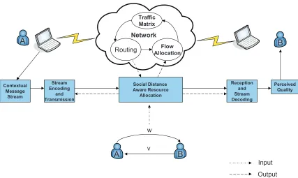
The scope of this work is limited to applying knowledge of social context between end users
to resource allocation decisions in the underlying network in order to improve the network
performance (Figure 1.4). The social context is not derived based on any traffic monitoring between end users of the network. In our work, social context is in fact represented through the
notion of social distance between users. The social distance is just a measure of the perceived
relative priorities of relationships (of a user) to him/her personally. We do not derive it from traffic intensity measurements, it is declared a-priori by the users themselves through choosing
values from a common reference scale of social distance. In our work related to studying social
relationships between content, social distance is correspondingly measured based on the relative popularity of content.
The network which we consider for our work is a wireless network, which works according to
Network
Contextual Message
Stream
Stream Encoding
and Transmission
Social Distance Aware Resource
Allocation
Reception and Stream Decoding
Perceived Quality
A B
A B
Routing AllocationFlow
Traffic Matrix
w
v
Input
Output
Figure 1.4: The scope of our work within the broader area of Traffic Engineering.
we consider the specific case of a IEEE 802.11e QBSS forming the underlying wireless network.
We focus on the case of a single collision domain with all communication happening through an access point (AP).
1.4.1 Objectives
The objectives of our work are as follows:
Service differentiation by social distance
Flows should be differentiated based on their associated social distance, in addition to their
traffic type. Traditional service differentiation algorithms classify flows solely based on the
Increase network performance
By allocating resources based on the added dimension of social distance (in addition to traffic
type), we intend to show that the network performance is improved for the same available
resources. The end user experience is in line with their expectations which is determined based on the associated social distance.
Real-time flows differentiation
In an IEEE 802.11e QBSS, there is an explicit priority for voice traffic over video. We intend
to classify all real-time flows based on the social distance associated with the flows instead of the traffic type, thereby ensuring a fair access to all real-time flows to the network.
Content distribution by social distance
Socially related content can be a good predictor of access patterns of end users. For the specific
case when the content is invariant (e.g., video), caching decisions are relevant and can improve the end user experience along with network performance. We look at the problem of determining
candidate content items for caching and distribution over the network.
1.5
Overview of Thesis
The thesis is organized as follows. In Chapter 2 we define the social distance associated with
end-users, and propose a way to measure the social distance for all users in the network. This
local measure of social distance is augmented with the global centrality measures of the end-users to derive a social-network-wide social distance measure. We define the generic form of a
social distance aware utility function, and provide examples for the case of elastic traffic. In Chapter 3 we look at the problem of determining a closed form expression for voice
call capacity in wireless networks. We do this in order to derive some notional bounds for
the maximum acceptable number of calls in a wireless network. Following this, in Chapter 4 we compare the performance of SDA with IEEE 802.11e QBSS for the case of voice calls. We
provide theoretical as well as simulation results which demonstrate that SDA achieves increased
network utility as compared to IEEE 802.11e for every case considered. In Chapter 5 we look at the case where voice and video calls are competing for the shared channel. We show that
SDA allocates resources based on the social distance rather than solely based on traffic type
(as is the case for IEEE 802.11e).
In Chapter 6, we look at the case where end users are accessing content hosted on the
network, and there are inter-relationships between the content items. In such a scenario, the
this for the case of three centrality measures (degree, closeness, betweenness), which are used
to compute the relative importance for individual content items and cache them. Through a future access list, we determine which of the three centrality measures provide the best cache
performance. Finally, in Chapter 7 we look at some of the applications that we implemented
Chapter 2
Social Networks and Social Distance
Users communicating through real-time flows over the network initiate those flows due to an underlying reason, acontext associated with the flow. The arrival of such flows into the network
is thus driven by the social interrelationships of a user, and the level of importance that he/she
attaches to them. The expected level of quality is also different for incoming flows depending on the social context. Consider, for example, an organizational network where the users are
categorized as managers and employees. Suppose that the users of this social network are
communicating with each other over a shared network using voice calls. When two concurrent voice calls are competing for resources, the social context can provide a good measure of relative
priority between the voice calls. For example, a call between two managers should be treated
as more important than a call between two employees. When several such users are competing for resources over a shared network, eliciting the underlying social context enables the network
to differentiate flows based on their real-world priorities irrespective of their traffic type.
In this chapter, we first provide a definition of social distance as used in this work. Social distance can be thought of as the edge weight (of a relationship) in the social graph. The
social graph is determined by users declaring their relationship peers along with the perceived
importance of these relationships (social distance) to them personally. All users identify the importance of their relationships using the same reference scale. This is done in order to keep the
notion of social distance simple. Through this information, we then generate a
social-network-wide social-distance measure, which combines the user’s personal preferences with their (the user’s) overall importance in the bigger social network. This is necessary to bring out the true
relative priority of the relationships when looked at from the social network perspective. We
illustrate this using a simple example of a social network. In order to incorporate social distance into resource allocation algorithms, we derive the generic form of a social distance aware utility
A B C D E F G H I 1 1 1 1 2 2 1 1 1 1 3 3 3 2 3 1 1 1 1 1 2 2 2 3 2 2 3 2
Figure 2.1: An example organizational social network. Each user identifies his/her peers and the perceived priority of the corresponding relationship to him/her personally.
2.1
Motivation
We define the context associated with a flow to be the social distance between the users initiating
that flow. This is motivated by the fact that most of our interactions through the network are
guided by our social interrelationships and their perceived importance. Knowledge of the social distance can aid the network in categorizing flows according to their real-world priority, rather
than solely based on the traffic type. At the macro level, traffic type based differentiation
still works for distinguishing real-time flows from non real-time flows. But at a microscopic level, such as looking at just the real-time flows in the network, we believe that social distance
provides a more reliable measure of priority determination as compared to the traffic type.
Social distance, as defined and used in Sociology, is variously used to measure both qual-itative [11][12] (degree of closeness, feeling of sympathy) as well as quantqual-itative (frequency of
interaction between social groups) information about an underlying social network. For our work, social distance is used to measure the relative priority or importance of a relationship
to a user. Each user identifies his/her relationships with other users in the network. The user
also provides a measure of theimportance of this relationship to him/her relative to all of their remaining relationships. This does not mean that for a high priority relationship, the frequency
of communication with this peer will always be high [4][13]. The social distance is used only
service rather than the traffic type. Thus, social distance is used as an indicator to the network
about the real-world priority associated with the flow.
Social distance can be used to optimize current communication protocols by making the
network aware of this implicit relative priority. In the next two sections we look at the case
where human users are communicating through the network, and present an example of how social distance can be used to improve resource allocation in such a scenario.
2.2
Social Distance
Communication between any two (human) end users of a network will, in most situations, be
determined first by the existence of a social relationship between them, and second by its weight in the bigger social network. The existence of a social relationship can be ascertained by an
explicit acknowledgement by the end users themselves. Each user a-priori declares all of his/her
peers in the social network. The mere existence of a relationship does not indicate frequency of communication. This is also why inferring a social network by observing traffic on the network
may not provide us with the real-world priorities of social relationships. Such an activity would
provide us with information about the traffic profile and hotspots, and aid in load balancing in the network. However, our goal is to differentiate between flows based on their real-world
priorities.
Along with the social relationships, end users will provide a measure of the perceived im-portance of the relationship tothem, personally. Since the perception may indeed be different
for peers of the same relationship (employee-manager), the resulting social graph is asymmet-ric. Each user will choose the social distance (importance) of the relationship from a common
reference scale. Since the user indicates distance of a peer to him/her, a smaller social
dis-tance denotes higher impordis-tance, and thus higher real-world priority. Thus, we need a common reference scale with a notion of closeness to define the social graph.
Definition Given a community overlay networkS, there exists a real number scaleζ together with a notion of closeness (or proximity) which can be used to define relationships. We can identify the relationship between a pair of communicating entities i and j in this community
overlay network by choosing a representative element χij ∈ ζ. We call this representative
elementχij thesocial distance between entitiesi andj.
The social distance scale ζ is common for all the users, and so is the definition of closeness.
In Figure 2.1 for example, the social distance scale is the set ζ = {1,2,3}, where 1 is the closest (highest priority) social relationship and 3 is the farthest (lowest priority). From this
information, we can distinguish between the relationships of a single user. However, when two
to differentiate between such flows. The priority of the relationship to the peers has been
ascertained, but its importance in the wider social network has still not been measured. We achieve this by including the centrality of the end users in the definition of the social distance.
2.2.1 Centrality and Social Distance
As the social network is usually represented as a graph (Figure 2.1), where the nodes are the
users and the edges represent relationships, centrality measures can be defined for nodes in the social network. In fact, social network analysis uses the centrality of a node to quantify
its relative importance in the social network, with a node having higher centrality perceived as being more important in the social network. Social networks are also known as scale free
networks, because a few nodes will have a high number of connections (called hubs). A centrality
measure helps identify such nodes, and hence the scale free nature of the graph itself.
There are several centrality measures defined in literature, such as degree, closeness,
be-tweenness [14][15][16][17]. We use one such measure called the eigenvector centrality. This
measure was proposed by Bonacich [18], and it is based on the idea that the eigenvector corre-sponding to largest eigenvalue of the adjacency matrix (of the social network) is a good measure
of the relative weights of nodes in the network. Eigenvector centrality measures the importance
of a node in terms of the centrality of its neighbors.
We compute the importance of nodes in Figure 2.1 by evaluating eigenvector centrality based
on the chosen relationship weights. This results in the hubs getting a higher centrality measure,
and delineating them from the rest of the users. The eigenvector centrality is computed by first determining all the eigenvalues for the adjacency matrix of Figure 2.1. The largest eigenvalue
is chosen, and the eigenvector corresponding to this eigenvalue is computed. This eigenvector
represents the relative weights of nodes in the social network.
For a given node, we now have two measures which we need to combine. First, the self
assessed (in isolation by the node) relationship distances, and second the eigenvector centrality
of the node. Continuing with the convention of a smaller social distance representing higher priority we define the network-wide social distance to be:
χIij = χ
i ij
Ci !
(2.1)
where, χiij is the self-assessed relationship weight by nodei,Ci is the eigenvector centrality
of node iand χIij is the corresponding global social distance measure for node i. We omit the
superscript onχij, and it is in factχIij which is being compared between competing flows. The
χ =
0 3.4 0 3.4 10.3 10.3 0 0 0
1.6 0 3.4 6.8 0 0 0 0 0
0 3.4 0 3.4 0 0 0 0 10.3
1.0 6.8 3.4 0 0 0 6.8 10.3 0
2.5 0 0 0 0 6.8 0 0 0
1.5 0 0 0 6.8 0 10.3 0 0
0 0 0 3.4 0 6.8 0 6.8 0
0 0 0 3.4 0 0 6.8 0 10.3
0 0 3.4 0 0 0 0 6.8 0
The distances in the matrix are normalized by the lowest value, which we take to be the
social distance 1. Note that the matrix reflects the two-tier nature of the graph. The nodes
index the rows of the matrix, from node A representing row 1, to node I representing row 9. Suppose there are two voice calls competing for resources in the network. Call 1 is being
requested by node A for node B. Call 2 is being requested by node F for node G. The social
distances for these calls can be found to be:
χ1 = min(χAB, χBA) = 1.6
χ2 = min(χF G, χGF) = 6.8
Summarizing, the users choose their perceived social distance to all their relationship peers in the network by selecting values from ζ. ζ is kept very simple, and is the same for all
the users of the network. Looking at these distances it would not be possible to identify the
relative priorities which exist at the global level due to the social network structure. We use the eigenvector centrality of the nodes to rank the users by importance, and compute the modified
social distance matrix. The values from this matrix can clearly bring out the scale free nature
of social network, and are used in the resource allocation algorithm for prioritization of flows.
2.3
Utility Optimization
Resource allocation problems in networks have been modeled in theory as utility optimization problems [19], with the objective being to optimize the total utility of the network. Utility
functions are defined for transport and application layer flows in terms of the network resources
allocated to them. They are a mapping from the resource set to the real number scale, with the value of the utility function denoting the relative profit to the flow. Several theoretical
utility functions have been defined in literature which achieve a particular objective [20] (e.g.,
problems [21].
Utility functions for real-time flows (voice and video) are interesting in that they are subjec-tive, that is they depend on the end user’s opinion about how they perceived the quality of the
flow. Thus, these utility functions are derived through user surveys based on several versions of
the received (and reconstructed) real-time flow. In defining our social distance aware resource allocation problem (SDA), we first look at a simple theoretical extension of the classical utility
maximization problem. We follow this up with a discussion of how the social distance aware
component of the modified utility function can be determined for real-time flows (since their utility is by definition subjective).
Let S denote the set of all flows in the network. Then the utility {Us|s∈S} is defined to
be,
Us : cs→R | cs ⊆NR (2.2)
where cs is the subset of network resourcesNRcurrently allocated to flow s. The utility is
usually a non-decreasing function of the resources allocated to the flow.
The classical network utility optimization problem (in the case of a wired network) for our example social network (Figure 2.1) is as follows:
maximize {cs}
X
s
Us(cs)
subject to X
s
cs≤NR (2.3)
Since the utility function of similar flows will be the same, resources are shared equally
among the flows without regard to the real-world priority of the flow. In a scenario where
the network resources are constrained, the resource allocation according to Problem 2.3 would not be optimal because all the competing flows lose resources equally, when in fact some of
them are at a lower priority than the others. Also, the solution to Problem 2.3 under current
service differentiation schemes (classifying by traffic type) would produce unfair allocations for scenarios where a high priority flow is using a non-high priority traffic type.
We therefore incorporate the social distance of a flow into the definition of its utility. One
way to achieve this is by introducing per-flow social distance dependent utility bounds, which restrict the maximum achievable utility of a flow with increasing resources. The idea behind
this is that by suitably modifying the maximum achievable utility (with increasing resources),
also be a bound on the minimum utility acceptable to the flow so as to create a threshold on
the received quality. We denote the maximum utility bound for flow s by Umaxs . This bound depends on the social distance of the flow. For lower social distances (high priority) the bound
will be high. The mathematical form of Umaxs is dependent on Us as well as χs. Thus, the
modified utility maximization problem can be defined as:
maximize {cs}
X
s
Us(cs)
subject to X
s
cs ≤NR
Us(cs)≤Umaxs (χs) (2.4)
This problem can be decomposed because the maximum utility bound constraint is a
per-flow constraint. Dual decomposition of this problem gives us the per-per-flow optimization problem to be:
maximize
cs
(Us(cs)−λ(Us(cs)−Umaxs (χs)))−µs(cs)
subject to cs∈C (2.5)
The utility function of the flow is now a function of both the resources allocated to it, as
well as the social distance associated with the flow. More generally, in order to incorporate the
social distance into resource allocation decisions at the network, we define a modified utility functionUbsfor flow swhich depends oncs as well asχs. Let flowsoriginate at nodeiand the
destination be nodej. Then the modified utility function takes the form,
b
Us(cs, χs) =Us(cs)−βf(χs, cs)
where χs= min(χij, χji) (2.6)
This social distance aware utility function can then inform the network of its ability to accept suboptimal resource allocations. Flows with higher social distances do not need the
highest resource allocation, and the acceptable allocations can be suboptimal with respect to
the original utility function Us. Through Ubs we make this fact explicit in the formulation,
thereby allowing the original solution algorithm to work without any change.
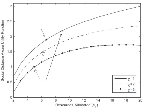
We now provide a generic example in order to illustrate how social distance affects the
2 4 6 8 10 12 14 16 18 20 0 0.5 1 1.5 2 2.5 3
Resources A llocated (cs)
S o c ia l D is ta n c e A w a re U ti li ty F u n c ti o n χ=1 χ=2 χ=3
Figure 2.2: Prioritized resource allocation among three flows of the same traffic type.
which results in proportionally fair resource allocation between the flows.
Us(cs) =log(cs) (2.7)
We consider n= 3 flows in the system. For the case of NR = 20, the optimal solution to
Problem 2.3 is cs = 6.67 for S = {s1, s2, s3}. Now consider the social network graph for the
users is such that χ(S) ={1,2,3}. We define the social distance aware utility function as,
b
Us(cs, χs) =log(cs)−0.5
(χs−1)
e−k
where k= 15−cs
2 (2.8)
Such a definition produces scaled utility functions for the same traffic type depending on
χs. The resulting utility functions and the optimal solutions for the three flows are shown
in Figure 2.2. The optimal allocation of resources for the three flows is evaluated to be
{8.87,6.21,4.92}. Compare this to the original optimal point for the three flows{6.67,6.67,6.67},
2.3.1 The function f
The choice of f is necessary to the definition of utility in terms of the social distance. By
looking at the form of Ucs (2.6) we know that f has to be convex in order for the modified
utility function to remain concave. The social distance matrix will remain constant for a much longer timescale than resource allocation decisions for the span of a flow. Thus, χs can be
assumed to be constant in f for a given flow (a specific source-destination pair). Equation
2.6 can be interpreted as reducing the incremental increase in utility for a unit increase in the allocated resources. Such a definition should produce different versions of the utility function
as shown in Figure 2.2. Thus, the exact definition of f in terms of cs and χs depends on Us,
and hence on the traffic type.
For the case of real-time flows, the utility functions are subjective measures dependent on
the perception of the end user about received quality. The mean opinion score for voice is one such utility function. Similar functions are defined for video traffic (e.g., peak signal to noise
ratio). The utility function is defined in terms of thresholds on received quality such as a mean
opinion score of 5 is excellent quality and so on. Such a utility function can also then be used to set bounds on expected quality at the receiver depending on the social distance. For example,
a call with higher social distance (lower priority) will demand received quality only up to a
mean opinion score of 4. Once the acceptable thresholds of the utility function are mapped to corresponding resource demands from the network, we can define f as the function which
achieves conversion from social distance to the expected utility bounds.
The assumption that we have such thresholds of the utility function is necessary to accom-modate inelastic traffic optimally. The reasoning is that maximizing resource allocation without
changing the utility threshold is of no use to the inelastic flow. It can do without the extra
resources and still achieve the same perceived quality at the receiver. The extra resources can then be allocated to other inelastic/elastic flows.
The definition of cUs also helps identify the real-world priority of flows irrespective of traffic
type. In wireless networks with a MAC layer capable of delivering quality of service (IEEE 802.11e QBSS), voice is prioritized higher than video traffic. This works to the detriment of
video flows when the system (QBSS) is working at capacity. Through social distance aware
utility functions for both voice and video, we can prioritize flows by their perceived importance rather than traffic type.
The choice of f is guided by the utility function of the flow, and by the mapping from
network resources to achievable utility. It will thus be different for each traffic type. It also depends on the social distance matrix of the network. We focus on the specific case of users
2.4
Social Distance in Content
The objective of end users accessing the network can broadly be either to communicate with
other users through real-time flows, or to receive content of their interest hosted on the network. For the case of content, the quality of service is determined by the transfer times needed to
deliver content to the user. This can be obviously improved for the case of invariant content
through replication and distribution at various levels in the network. It is thus important to determine the probability of access for content in order to bring it closer to end users.
Relationships between content data have been used to determine the importance and
rele-vance of individual datum (e.g., web pages) within the content space. This is the predominant feature of search algorithms which rank web pages based on the weight of links which refer to
them (incoming links). With the increasing popularity of social media (e.g., Youtube), such relationships between content are now explicit. The set of relationships can actually be used
to determine the user’s future access patterns. In the case of video content, the data does not
change over time and thus is suitable for caching at various levels in the network. The decision to bring content closer to the user is also a part of Traffic Engineering, since it improves the
end user’s experience of the network without changing his/her access network’s resources.
2.4.1 Rank Distribution
The characteristics of user access patterns about related video content, especially for the case of Youtube, have been studied in literature [22][23]. The properties of rank distributions (access
counts) for video items have also been studied [24], and compared to the Zipf distribution
which has been shown to be applicable to web pages. It is this property of web pages (Zipf distribution) which makes caching attractive.
There are publicly available data traces about Youtube content [25] for videos belonging to particular “categories” in Youtube. We look at the feasibility of caching for video data by
studying the rank distributions of the available data traces. The two categories for which traces
have been made available are the Science and Technology category, and the Entertainment category.
In the data traces, for each video, information about its popularity, rating, size, duration
and several other properties are compiled. We extract the number of views properties for all the videos in these traces to determine the rank distributions for these videos. The results are
shown in Figure 2.3. Videos are ranked starting from 1, with the video with the highest number
of views ranked as 1. The rank distribution follows power law, which is a characteristic of social networks. It is close to Zipf distribution for static web pages, except that the tail of the curve
tapers off exponentially.
Figure 2.3: Rank distributions for two categories of Youtube videos.
and thus video content is suitable for caching. We determine the social distance between related videos by making it inversely proportional to the popularity of a video. Thus, a highly popular
video file will have low cost edges from all its neighbors. The result of this is a social network
of videos, structured by social distances which are in turn determined by the popularity of individual videos.
2.4.2 Content Caching and Distribution
For the case of invariant content, distribution and caching of content can improve the network performance by reducing repetitive requests over the network for the same content. It can also
improve the perceived end user experience of the network by bringing the content closer to the
user, and thus reducing transfer times without changing anything in the user’s access network. We focus on the problem of identifying important content in Chapter 6, and evaluate different
centrality measures in terms of their effectiveness in identifying the most queried content over
the network.
2.5
Summary
In this chapter, we proposed a way to measure the social distance between users by determining
can be generated by combining the user’s preferences with his/her overall importance in the
wider social network. The importance of a user is measured in terms of his/her eigenvector centrality.
We then incorporated the social distance measure into the definition of utility function for
a communication flow. We initially demonstrated how this could be done through imposing social distance aware utility bounds on flows, and then provided a generic definition of a social
distance aware utility function. We also provide an example of social distance aware resource
allocation for the case of elastic traffic.
Finally, we looked at the case of social distance between content, and how this can be used
to study the relevance/popularity of content in the content space. We showed rank distributions
for the case of publicly available data traces for Youtube videos, which demonstrate that video content access also follows the Zipf distribution for the popular videos. This means that the
content is a good candidate for caching and distribution, which can be used to improve network
Chapter 3
Voice Call Capacity Analysis
The original IEEE 802.11 standard for a wireless LAN did not have any capability to provide differentiated services to real-time flows. It is only through the IEEE 802.11e extension to
the original standard that such service differentiation can be achieved between flows of differing
traffic types. Accommodating real-time flows into a wireless network while meeting their quality of service requirements necessitates the need for estimating capacity of wireless networks for
such real-time flows. Unless there is a way to measure when the capacity will be reached, or
at least to predict how many flows can be concurrently accommodated while meeting their individual service requirements, some of the flows will fail. Thus, capacity analysis of a wireless
network can help provide theoretical thresholds for the number of concurrent real-time flows
which can be accommodated.
In this chapter, we look at the problem of developing a closed form equation for wireless
channel capacity, for the specific case of voice traffic. It is important to have an estimate of the
number of voice calls that can be accommodated in a wireless network such that all the calls receive acceptable service (mean opinion score). We do this for the case of the standard IEEE
802.11b wireless LAN with a maximum data rate of 11Mbps.
The channel capacity will differ based on the achieved data rate of the channel, as well as the source coding which is used for voice calls. We define the voice call capacity of the channel
in terms of these variables, and perform simulations for every combination of the variables to
determine the achieved call capacity. We then fit the data to our proposed model using linear regression fitting. Using the closed form equation for capacity, we determine the degree of
dependence of voice call capacity on the chosen source coding. An explicit knowledge of how
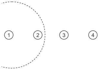
1 2 3 4
Figure 3.1: The simple chain topology used for our simulations.
3.1
Background
In the literature, voice call capacity has been studied for different wireless network
configura-tions, specifically for the case of a wireless mesh network [26][27]. The focus of these works is on performance optimizations for voice calls such as packet aggregation and header compression
for improving the capacity in the case of wireless mesh networks. Another related work [28]
deals with the challenges faced by voice calls at different layers of the protocol stack – MAC layer, routing layer and mobility management. There are also studies which look at the QoS
challenges and pitfalls for wireless mesh networks based on the 802.16 mesh mode [29].
In a related previous work [30], the authors had looked at the effect of the Wireless LAN on
the voice service. Response surface modeling methodology was applied to derive the throughput
and voice call capacity for Wireless LAN’s. In a later work [31], an extended model which took into account cross layer interactions through layer interface parameters was proposed.
3.2
Simulation Setup
We use the simple chain topology for our simulations (Figure 3.1), with number of hops varying from 1 to 3. The distance between nodes is set to be 250m, and the transmission range is set to
be slightly greater than 250m. There are mainly two parameters of interest in determining the
voice call capacity. They are the channel data rate, and the voice call packetization interval. The channel data rate is set to be one of{1,2,5.5,11}. For a nhop topology, this gives us 4n
possible combinations.
The second parameter of interest is the voice packetization interval. We use the G.711 codec
for voice calls [32], which is the pulse code modulation standard for voice traffic. Voice calls
This is the basic packetization interval (10ms). It can be changed so as to aggregate more voice
samples into the same packet, and such a choice sets up a tradeoff between delay and packet loss. For high packetization intervals, loss of a single packet can result in a significant loss of
quality. We vary the packetization interval between 10ms to 100ms for our simulations, which
results in a total of 10 possible combinations for voice calls. The relation between packetization interval and the packet stream generated is as follows:
PI = 0.01∗k, 1≤k <10
PacketSize = 80∗k bytes
IARate = 0.01∗k (3.1)
where PI represents the chosen packetization interval, and IARate is the inter-arrival rate
for voice packets.
The voice traffic is generated using CBR traffic generator in ns-2 with the parameters given by Eq. 3.1, with the duration of the voice calls set to be 3 minutes. We compute the achieved
QoS of a given voice call through the mean opinion score. In order to do this, we first compute
the R-value of the call [33], and then translate it to the mean opinion score [34].
Starting from a single voice call, we increase the number of calls until at least one call
fails. We do this for every combination of data-rate and packetization interval. At the end of
the simulations we have the set of system responses for all the different combinations of input parameters. This data forms the input to the SAS GLM procedure to derive the metamodels
for call capacity.
3.3
Call Capacity Models
In order to determine voice call capacity models, we first formulate a generic function in terms
of all the chosen system variables (which were varied during the simulation). The call capacity of a wireless channel is a non-linear function of our chosen variables, mainly due to the shared
broadcast channel coupled with the exponential backoff mechanism. In order to apply linear
regression fitting for our proposed call capacity functions (with the simulation data), we trans-form the variables. We use the natural logarithm of the variables in place of the variable itself,
3.3.1 Single Hop Wireless Network
This is the equivalent of the downlink from an AP to the station, and thus determines the
capacity of the maximum capacity of the downlink in the absence of any interfering flows. There
are only two variables in this scenario, the channel data rate (x1) and the voice packetization
interval (x2). We define the following sets for easy characterization of these variables:
D = {1,2,5.5,11} (3.2)
P I = {0.01∗k | 1≤k <10} (3.3)
I1 = {1,2} (3.4)
Now we can define our variables to bex1∈D, andx2∈P I. The voice call capacity is defined
in terms ofx1 and x2 as:
N = β0+
X
i∈I1
βiln(xi) + X
i,j∈I1,j>i
β(i+j)ln(xi)ln(xj) (3.5)
We obtain an estimate of the beta’s from SAS GLM, and the fitted values are shown in Eq. 3.6.
The ANOVAR-square measure for this fit is 0.987911. A value closer to 1 is desired, and thus
this is a good fit for the voice call capacity.
β0 = 20.203, β1 = 28.490
β2 = 3.728, β3 = 6.724 (3.6)
3.3.2 Two Hop Wireless Network
This is representative of a single collision domain wireless network (with reference to the AP), where communication between clients is achieved through the AP. In this case, we have two
link data rates to consider. We represent these by x1 and x2. The packetization interval is
represented byx3. The variables can be defined as,x1∈D,x2∈Dandx3 ∈P I (Eq. 3.4). We
define the following set, I2={1,2,3}. The function for voice call capacity is of the form:
N =β0+
X
i∈I2
βiln(xi) + X
i,j∈I2,j>i
β(i+j+1)ln(xi)ln(xj)
+ X
i,j,k∈I2,k>j>i
0 2 4 6 8 10 12 0 0.02 0.04 0.06 0.08 0.1 0 5 10 15 20 25 Datarate (Mbps) Packetization interval (ms)
Number of Calls
(a):
0
5
10
15
0.01 0.02 0.03 0.04 0.05 0.06 0.07 0.08 0.09 0.1 0.11
0 2 4 6 8 10 12 14
Packetization interval (ms) Data rate (Mbps)
Number of calls
R2=1Mbps R2=2Mbps R2=5.5Mbps R2=11Mbps
(b):
Figure 3.2: System Response for 2 Hops (Figure 3.2a) and 3 Hops (Figure 3.2b) are shown. For both cases, one of the links is set to have the data rate of 11Mbps, while the other data rates are varied.
From the SAS GLM procedure, we obtain an estimate of the beta’s which are shown in
Eq. 3.8. The ANOVAR-square measure for this fit is 0.980833.
β0 = 12.339, β1= 2.983, β2 = 3.114, β3 = 2.531
β4 = 3.639, β5 = 0.638, β6= 0.669, β7 = 0.875 (3.8)
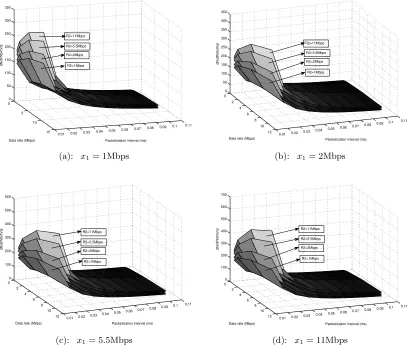
3.3.3 Three Hop Wireless Network
In this scenario, we have 3 link data rates as part of the variables. These are represented
by x1,x2,x3 respectively. The packetization interval is represented by x4. The variables are
defined as follows: x1, x2, x3 ∈ D, x4 ∈ P I (Eq. 3.4). The new variable set is defined to be
I3 ={1,2,3,4}. The function for voice call capacity is of the form:
N =β0+
X
i∈I3
βiln(xi) + X
i,j∈I3,j>i
β(i,j)ln(xi)ln(xj)
+ X
i,j,k∈I3,k>j>i
β(i,j,k)ln(xi)ln(xj)ln(xk)
+ X
i,j,k,l∈I3,l>k>j>i
0
5
10
15
0.01 0.02 0.03 0.04 0.05 0.06 0.07 0.08 0.09 0.1 0.11 0 50 100 150 200 250 300 350
Packetization interval (ms) Data rate (Mbps)
dN/dPktIntVal
R2=5.5Mbps
R2=2Mbps
R2=1Mbps R2=11Mbps
(a): x1= 1Mbps
0 2 4 6 8 10
12 0.01 0.02 0.03 0.04 0.05 0.06 0.07 0.08 0.09 0.1 0.11 0 50 100 150 200 250 300 350 400 450
Packetization interval (ms) Data rate (Mbps)
dN/dPktIntVal
R2=5.5Mbps
R2=2Mbps
R2=1Mbps R2=11Mbps
(b): x1= 2Mbps
0 2 4 6 8 10
12 0.01 0.02 0.03 0.04 0.05 0.06 0.07 0.08 0.09 0.1 0.11 0 100 200 300 400 500 600
Packetization interval (ms) Data rate (Mbps)
dN/dPktIntVal
R2=11Mbps
R2=5.5Mbps
R2=2Mbps
R2=1Mbps
(c): x1= 5.5Mbps
0 2 4 6 8 10
12 0.01 0.02 0.03 0.04 0.05 0.06 0.07 0.08 0.09 0.1 0.11 0 100 200 300 400 500 600 700
Packetization interval (ms) Data rate (Mbps)
dN/dPktIntVal
R2=11Mbps
R2=5.5Mbps
R2=2Mbps
R2=1Mbps
(d): x1= 11Mbps
Figure 3.3: Partial derivatives of the call capacity (for 3 hops) with respect to the packetization interval.
From the SAS GLM procedure, we obtain an estimate of the beta’s which are shown in Eq. 3.10. The ANOVAR-square measure for this fit is 0.972616.
β0= 7.335, β1 = 0.898, β2 = 0.905, β3= 1.393, β4= 1.516, β1,2 = 0.256
β1,3= 0.202, β1,4 = 0.205, β2,3= 0.517, β2,4 = 0.534, β3,4 = 0.303, β1,2,3 = 0.504