The maintenance of genetic variability in two-locus models of stabilizing selection.

(1)

The Maintenance

of

Genetic Variability in Two-Locus Models

of Stabilizing Selection

Thomas Nagylaki

Department of Molecular Genetics and Cell Biology, The University of Chicago, Chicago, Illinois 60637 Manuscript received September 20, 1988

Accepted for publication February 6, 1989

ABSTRACT

T h e maintenance of genetic variability at two diallelic loci under stabilizing selection is investigated. Generations are discrete and nonoverlapping; mating is random; mutation and random genetic drift are absent; selection operates only through viability differences. T h e determination of the genotypic values is purely additive. T h e fitness function has its optimum at the value of the double heterozygote and decreases monotonically and symmetrically from its optimum, but is otherwise arbitrary. T h e resulting fitness scheme is identical to the symmetric viability model. Linkage disequilibrium is neglected, but the results are otherwise exact. Explicit formulas are found for all the equilibria, and explicit conditions are derived for their existence and stability. A complete classification of the six possible global convergence patterns is presented. In addition to the symmetric equilibrium (with gene frequency 1/2 at both loci), a pair of unsymmetric equilibria may exist; the latter are usually, but not always, unstable. If the ratio of the effect of the major locus to that of the minor one exceeds a critical value, both loci will be stably polymorphic. If selection is weak at the minor locus, the more rapidly the fitness function decreases near the optimum, the lower is this critical value; for rapidly decreasing fitness functions, the critical value is close to one. If the fitness function is smooth at the optimum, then a stable polymorphism exists at both loci only if selection is strong at the major locus.

T

HE maintenance of genetic variability in quanti-

tative characters is of fundamental evolutionary importance. T h e mechanism proposed most widely in studies of this question is the balance between muta-

tion and stabilizing selection. Consult BARTON (1 986),

BARTON and TURELLI (1987), BURGER (1986, 1988,

1989), NARAIN and CHAKRABORTY (1987), SLATKIN

(1987), and TACHIDA and COCKERHAM (1988) for

recent investigations and references to the earlier

work of BULMER, FLEMING, KIMURA, LANDE, LATTER,

and TURELLI.

Stabilizing selection toward an intermediate phenotypic optimum has been established for many quantitative characters in natural populations (ENDLER

1986, Ch. 7). Mutation is incorporated because several analyses suggest that stabilizing selection tends to re- duce genetic variability in polygenic traits. This view is supported by approximations that focus on a single

locus at a time (FISHER 1930, Ch. 5; ROBERTSON 1956;

BULMER 197 1; KIMURA 1981; NAGYLAKI 1984).

WRIGHT’S (1935) study of the quadratic optimum model for diallelic loci without epistasis in the determination of the character provides additional support. He neglected linkage disequilibrium and found that

at most one locus could be in stable polymorphic

equilibrium if dominance was either absent or complete. For two loci with equal effects, complete addi- tivity, arbitrary recombination rate, and an arbitrary symmetric fitness function with optimum at the value

Genetics 122: 235-248 (May, 1989)

of the double heterozygote, HASTINGS (1987) proved

that both loci are ultimately fixed.

Stable multilocus polymorphisms can occur in the quadratic optimum model even with equal contribu-

tions if there is partial dominance (KOJIMA 1959;

LEWONTIN 1964; SINGH and LEWONTIN 1966), epis-

tasis (A. GIMELFARB, unpublished manuscript), or

pleiotropy for two characters (GIMELFARB 1986). T h e

combination of stabilizing selection and viability overdominance can also maintain genetic variation (BUL-

MER 1973; GILLESPIE 1984).

In all the investigations of mutation-selection bal-

ance cited above, it is assumed that the trait is deter-

mined without dominance or epistasis. Therefore,

numerical work of GALE and KEARSEY (1968), and

KEARSEY and GALE (1 968) on completely additive two-

and three-locus models of pure stabilizing selection is

of particular interest. In contrast to the commonly

posited quadratic or Gaussian fitness functions, these

authors used a triangular one (ie., one that decreases

linearly from its optimum). They found that all the

loci can be stably polymorphic if their effects are

sufficiently unequal, and that the amount of disparity required decreases as linkage becomes tighter. How- ever, they did not incorporate a parameter to control the intensity of selection. Since selection is strong in all their examples, even the ones with loose linkage exhibit considerable linkage disequilibrium.

(2)

236 T. Nagylaki

SEY (1968) still leave open the questions of the de-

pendence of the possibility of stable multilocus polymorphism on the intensity of stabilizing selection and on the form of the fitness function. These questions will be answered for two loci in this paper.

We shall see that our fitness scheme is identical to

the symmetric viability model. By neglecting linkage

disequilibrium, we shall obtain a complete global

analysis, which complements the exact, local results of

BODMER and FELSENSTEIN (1967) and KARLIN and

FELDMAN (1 970) on this model.

In the next section, we formulate our model and

establish some preliminary results. In the following section, we present explicit formulas for all the equilibria and explicit conditions for their existence and stability. These results provide a complete classification of the six possible global convergence patterns

and are proved in the APPENDIX. In the succeeding

section, we examine how the amount of disparity

between loci and the form of the fitness function affect

the maintenance of genetic diversity. Then we treat some specific fitness functions. In the final section, we

summarize our main results and discuss extensions

and further applications.

FORMULATION

We assume that generations are discrete and nonoverlapping, mating is random, mutation and random genetic drift are absent, and selection operates only through viability differences.

Our sole approximation is to neglect linkage disequilibrium. Suppose that the genotypic fitnesses are

constant and there is no position effect: there are

arbitrarily many alleles at each of n loci. Let

pj')

and

wiljl,. . .,in,n denote the frequency of the allele Acj) at

locus

i

and the fitness of the genotype A\:)At)

.

A t ) A t ) . Then the mean fitness reads

5 =

C

wilj,...,,injn

Il

P t h P l h , ( 4 (4 (1) il.jl....,in,3n k

which is a polynomial of degree 2 n . T h e gene fre-

quencies in the next generation are given by

where all allelic frequencies are treated as independent in the partial differentiation. From the inequality

of BAUM and EAGON (1 967) we conclude immediately

that the mean fitness is nondecreasing:

zir'

2 5, with

equality only at equilibrium. Hence, in this approxi-

mation, locating all the stationary points of zir and

determining whether they are maxima provides a

global analysis of the evolution of the population. We specialize now to two diallelic loci. T h e linkage- equilibrium approximation is accurate for the situa-

TABLE 1

The genotypic values

BB Bb bb

AA d + c C - d + c

Aa d 0 -d

aa d - c -C -d

-

c

d ? c > O .

TABLE 2

The genotypic fitnesses

BB Bb bb

AA 1 - 6 1 - P 1-01

A a 1-7 1 _1-7

a a 1-01 _{1 - 0} 1 - 6

O s a , p s 7 < 6 s 1 .

tion of most biological interest, weak selection

(NAGYLAKI 1976; 1977a, pp. 167-177; 1977b). T h e

computations of SINGH and LEWONTIN (1966) and

GIMELFARB (1 986, unpublished manuscript) and com-

parison of our results with those of GALE and KEARSEY

(1 968) suggest that the inclusion of linkage disequili-

brium would relax the conditions for the existence of stable two-locus polymorphism without changing them qualitatively.

Simplifying the notation, we call the alleles A and a

at the first locus and B and b at the second. Let p l , 91,

p 2 , and 42 designate the frequencies of A, a , B , and b,

respectively. T h e alleles determine the genotypic

value, z, purely additively; without loss of generality,

we parametrize the contributions of A , a, B , and b to

z as Y2c, -1/2c, Yzd, and -?hd and take d 2 c

>

0. Thus, we obtain the genotypic values shown in Table 1. We

call c and d the effects of the minor and major loci,

respectively.

We assume that the genotypic fitnesses depend only

on the genotypic value and write them as w(z). We

posit that the fitness function w ( z ) has its optimum at

zero, the genotypic value of the double heterozygote: we scale w ( z ) so that w ( 0 ) = 1. We suppose that w ( z )

decreases monotonically from its optimum and is

even, w(-z) = w ( z ) . Henceforth, we shall write w ( z )

only for z L 0; replacing z by

I

z

I would always produce

expressions valid for --OO

<

z

<

m. With these hy-

potheses, the genotypic values in Table 1 yield the

fitness scheme in Table

2,

where

a = 1

-

w(d

-

c ) ,

/3

= 1 - w ( c ) , ( 3 4

y = 1 - w ( d ) , 6 = 1

-

w(d

+

c ) ; (3b)

O I a , p s y < 6 s l . (4)

We shall repeatedly utilize the simple fact that a

>

p

(3)

T h e fitness scheme in Table 2 is identical to the

symmetric viability model (BODMER and FELSENSTEIN

1967; KARLIN and FELDMAN 1970). Given c and d

such that d L c

>

0 and a ,

0,

y , and 6 satisfying (4),

there exist infinitely many nonnegative, nonincreasing

w ( z ) that pass through the points (0, l), ( d

-

c , 1

-

a ) , (c, 1 - @), ( d , 1

-

y ) , and ( d

+

c , 1

-

6).

Our fitness scheme is symmetric under the simul-

taneous interchanges A t,a and B c, b, which corre-

spond to

pl

t,q1 and

p2

t,q 2 , respectively. Therefore,

every convergence pattern in the p1p2-plane is sym-

metric under reflection in the point

(Vz,

?h). In partic-

ular, excluding the equilibrium (%, %), the equilibria

must occur in pairs ( P I , p2) and (91, 42).

We shall see that if selection is weak at the minor locus, the possible convergence patterns depend on

the behavior of w ( z ) near the origin. This behavior,

in turn, depends on what smoothness hypotheses, if

any, we impose on w ( z ) . Although we shall impose

none, it is important to see that w ( z ) must be smooth

(i.e., have infinitely many continuous derivatives) under the following set of conditions. Suppose the phenotypic value is the sum of the genotypic value and a stochastically independent environmental contribu- tion. Then the genotypic fitness function can be writ- ten as

where Wand represent, respectively, the phenotypic

fitness function and the probability density of the

environmental value. If W ( z ) decreases sufficiently

rapidly as

I

z

I

-+ OQ to be integrable from --QJ to OQ and

4

is smooth (e.g., Gaussian), then w is smooth (APOSTOL

1974, p. 3 2 8 ) . Thus, smooth w ( z ) are of particular

biological interest.

GENERAL RESULTS

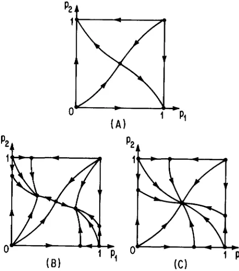
In this section, we locate all the equilibria and present conditions for their stability. This enables us

to classify the six possible global convergence patterns,

as shown in Table 3 and Figure 1 below. We state our

major results as theorems and prove them in the

We define first some parameter combinations that

APPENDIX.

greatly simplify our formulas:

1 = 6 + a , m = 6 - a , (6a)

X =

I

-

2p, P =

2(r

-

@), _(6b)

f

= ! h ( 1

-

p ) , h = Yz(1

+

p ) , ( 7 4

g = 2 ( 2 y

-

X). (7b)

[In BODMER and FELSENSTEIN (1 967) and KARLIN and

FELDMAN ( 1 970), 1 denotes 27

-

X , not 6

+

a.] These

parameters satisfy some useful inequalities. Subtract-

ing @ from (4) and employing (6a) and (6b), we find

max(0, X

-

m ) 5 p

<

X

+

m ; ( 8 4

in particular,

X

>

-m. (8b)

From (6) and (8b) we deduce the bidirectional implications

If X

>

0 , we can establish

2 > p - w X - 2 @ > € ( 8 4

by using (6) to prove that both inequalities in (8d) are

equivalent to m2

>

~ B X .

Clearly, the four vertices (0, 0), (1, l ) , (1, 0), and (0, 1) of the unit square in the p$2-plane are equilibria. We define

p1= ( ( 0 , O ) , (1, I)), p2 = ((1, O ) , (0, 1)). (9)

A glance at Table 2 informs us that there exist no

edge equilibria if a 5

P ,

whereas there exist the two

overdominant ones,

p 1 = 0 ,

p

- - + - > - ,

2 - 2 2X 2 (loa)

l m l

if a

>

P;

we call these P,. Note that (10) satisfies the

reflection symmetry

(pl, PP)

t,(41, q2), as it must. By

the same symmetry, the point Po =

(Yz,

%) is an

equilibrium. T o specify the unsymmetric internal equilibria, set

so that -?h I x , y I %.

Theorem 1: (i) Suppose g f 0 . A pair of unsymmetric internal equilibria, P+, given by

y =

-

G.,

exists in Cases a, b, and c in Table 3, but not otherwise. (ii) Suppose g = 0. The line of equilibria

=

-xx

(4)

TABLE 3

Classification of the convergence patterns and the existence and stability of the equilibria

Equilibria

Case Conditions p , Pe PC Po P ,

a e > p p < p 2

u

s

b c < p p > p 2 a s p U S -

s

u

c c < p p > p 2 a > p

u

s s

u

d c < p ' p < p 2 a s p U S -

u

-e e < p p < p 2 a > @

u u

s

u

-

f c > p p > p 2

u

s -

T h e parameters are defined in Equation 6. P I , P 2 , PC, Po, and P,

designate the vertices (0, 0) and (1, l), the vertices (1, 0) and (0, l ) , the two edge equilibria (lo), the symmetric equilibrium (%, Yz), and the two unsymmetric equilibria (12), respectively. T h e dash, S , and U signify nonexistence, stability, and instability of an equilibrium, respectively. Figure 1 shows the global convergence patterns for the six cases.

exists i f a n d only i f p = p2, which is equivalent to

a = P + y - & , S = / ? + y + & . (14) In Table 3, Cases d, e, and f complement Cases a, b, and c, excluding the degenerate cases of equality

E = p and p = p2. Notice that, by (8a) and ( 8 c ) , in Cases

a and f a

>

0,

which is equivalent to d

>

2c. T h e full significance of our classification follows from the conditions for stability of the equilibria, which we proceed

to consider. We abbreviate asymptotic stability as stabil-

ity. Let t designate time in generations.

Table

2

and (4) inform us that, as t + m, p l ( t ) + 1

along p 2 = 0 and p l ( t ) -+ 0 along p 2 = 1. Similarly, if

a! I /?, p , ( t ) + 1 along f i l = 0 and p , ( t ) + 0 along

P I

= 1. If a!

>

0,

p2(t) converges along

P I

= 0 to the edge

equilibrium (loa) and along f i l = 1 to (lob). We

conclude that the equilibria (0,O) and (1, 1) are always

unstable, whereas (1, 0) and (0, 1) are stable if a 5

0

and unstable if a

>

0.

Our next theorem concerns the stability of the edge

equilibria (1 0), which exist if and only if a!

>

0.

Theorem 2: Suppose a

>

0.

The edge equilibria (10) are stable i f t

<

p and unstable if€

>

p. In the degenerate case t = p, they are stable i f g

<

0 and unstable i f g

>

0.

T h e stability of the symmetry point ('h, !h), at which

the genetic variance is maximized, is of particular

interest.

Theorem 3: The symmetric equilibrium (%, 'h) is stable

i f p

>

p 2 and unstable $ p p 2 .

Thus, each of the three conditions in Table 3 has

an immediate meaning. As we proved below ( 2 ) , the

mean fitness is nondecreasing. Therefore, in nonde-

generate cases, the gene frequencies must converge

to some equilibrium point from all initial conditions,

and this enables us to determine the stability of the

unsymmetric interior equilibria (12) from that of the

other equilibria. In this manner, we obtain the six global convergence patterns shown in Figure 1 , cor- responding to the six cases in Table 3.

Several features of Table 3 and Figure 1 are inter-

esting. If there is a stable internal equilibrium, it is

either Po, the symmetric one (Cases b, c, and f ) , or

P+, the pair of unsymmetric ones (Case a). If P+ exists,

its stability is opposite to that of Po. There exists at

least one stable internal equilibrium in Cases a, b, c,

and f, but the two-locus polymorphism is protected

only in Cases a and f. Thus, protection is sufficient,

but not necessary, for the existence of a stable internal equilibrium. Moreover, in Cases a and f, as we noted

below (14), d

>

2c, which means that a substantial

disparity between the effects of the major and minor

loci is necessary, but not sufficient, for protection.

Finally, observe that stable internal equilibria are max-

ima of the mean fitness

W ,

unstable internal equilibria

are saddle points, and internal minima do not exist.

MORAN (1 963) proved for two independent diallelic

loci with arbitrary fitnesses that, excluding degenerate cases, there exist at most five internal equilibria, of which at most three are stable, and he offered examples in which these bounds are attained. KARLIN and

FELDMAN (1 970) demonstrated that as many as seven

internal equilibria can exist simultaneously in the ex-

act symmetric viability model, and HASTINGS (1985)

proved that four of these can be simultaneously stable.

Figure 1 establishes that with independent loci, at

least under the restriction (4), the generic number of internal equilibria in the symmetric viability model is

either one or three, and the number of stable internal

equilibria is 0, 1 , or 2.

We shall see that Case a seems to occur very rarely. When can it be excluded analytically? In the course of proving Theorem 1, we shall demonstrate that Case

a cannot occur if g

>

0. If several fitness functions

w,(z) satisfy our restrictions (normalization, monoton-

icity, and symmetry), then so does the fitness function

w ( z ) =

C

a,wi(z), a, = 1, (1 5)

1 I

where the ai represent positive constants. For each i ,

we define our parameters by subscripting (3), (6), and

(7). Then we calculate a!,

0,

y, and 6 by averaging as

in (1 5); since (6a) and (7b) are linear, we get

g =

2 aigi.

(1 6)

2

Consequently, if g,

>

0 for every i , then g

>

0. This result helps to exclude Case a for some fitness functions.

Let us prove next that g

> 0, and hence Case

a

cannot occur, if w ( z ) is convex for z 2 0. For all Z I Z

0 and z2 z 0 we have

(5)

Stabilizing Selection

( a )

p24

P24

Taking z1 = d

+

c and z2 = d

-

c in (17) and recalling

(3) and (6a), we find 1 I 27; in view of (6b) and (7b),

this implies that g L 4P

>

0.

We summarize the conclusions of the last two par- agraphs in the following proposition. We shall demonstrate by example below (55) that the conditions of Proposition 1 are not necessary.

Proposition 1: (i)

I f g

>

0, Case a cannot occur. (ii) I f

w(z) is given by (15) and g,

>

0 f o r each i, then g

>

0. (iii)

If

w(z) is convex for ,z 2 0, then g

>

0.

We devote the next two sections to extracting the implications of the above general results.

ASYMPTOTIC RESULTS

For each fitness function w ( z ) , the line d = 2c and

the boundary curves E = p and c~ = p2 divide the wedge

d L c

>

0 into at most six regions, each of which

corresponds to one of the cases in Table 3. In the

next section, we shall exhibit such case maps for some particular fitness functions. Here, we derive general features of case maps in proximate and distal regions

of the wedge d L c

>

0 by treating successively (i)

equal effects (c = d ) , (ii) strong selection at the major

locus ( d + with c fixed), (iii) weak selection at the

minor locus ( c + 0 with d fixed), (iv) weak selection

at both loci (0

<

c 5 d + 0), and (v) strong selection

at both loci ( d 2 c + w). If we scale z so that w ( z )

=

1 for

IzI

<<

1 and w ( z )

<<

1 for

IzI

>>

1, then we can approximate the limits (ii), (iii), (iv), and (v) by d

>>

1, c

<<

1 , 0 < c s d

<<

1, and d 2 c

>>

1, respectively.

Equal effects: If the two loci contribute equally to the character, i . e . , c = d , then (3) yields a = 0 and /3

= 7 . Hence, (6) and (8c) give 1 = m = 6, p = 0, c~

<

0,

FIGURE 1 .-The six possible convergence patterns for the symmetric viability model with independent loci. The coordinates are the gene frequencies at the two loci.

and E

<

0. We infer from Table 3 that Case d and

Figure I d apply. Consequently, on account of the biological ubiquity of small perturbations, the popu-

lation converges to either (1, 0) or (0, l ) , i.e., ulti-

mately the sole genotype in the population is either

AAbb or aaBB.

HASTINGS (1987) proved this result in the exact

model with linkage.

Strong selection at the major locus: We assume

that w ( z ) + 0 as z

-

co and let d + with c fixed.

From (3), (6), and (7b), we get a , 7, 6 + 1, 1 + 2, m

+ 0, p + 2(1

-

B),

p + 4, and E +

2 .

Therefore,

Table 3 tells us that Case f applies in this limit. Thus,

Po is globally stable if selection at the major locus is

sufficiently strong. This result is intuitively reasona- ble: in the limit, all the fitnesses in the first and third

columns of Table

2

are zero, so ($4,

1/2)

is the globally

stable equilibrium.

Our conclusion here seems to disagree with

WRIGHT'S (1935) result that at most one locus can be

in stable polymorphic equilibrium for the quadratic fitness function. T h e apparent discrepancy is resolved

by noting that for the quadratic fitness function (which

we shall examine in the next section), the nonnegativ-

ity of w ( z ) imposes an upper bound on d , so one cannot

let d + W.

Weak selection at the minor locus: We let c + 0

with d fixed. Assume that w ( z ) has at least three

continuous derivatives for z

>

0 and

W ( Z ) = 1 - kz"

+

o(z") (18)

as z + 0+, where

k

>

0 and K

>

0 designate constants.

By the argument below ( 5 ) , fitness functions that are

smooth even at the origin are especially important.

(6)

TABLE 4

Classification of the convergence patterns for small minor-locus effect

Conditions Case

K < 2 f

K = 2 vck f

K = 2 v > k e K > 2 V C O f K > 2 1 4 0 e

T h e parameters are defined in (18), (20), and (22).

expect K = 2, as for the Gaussian fitness function.

Employing (18) and Taylor's theorem in ( 3 ) , we de-

duce

a =

-

uc

-

7 c 2

+

0 ( ~ 3 ) , ( 1 9 4

6 =

+

uc

-

7 c 2

+

0 ( ~ 3 ) (1 9 4

/3

= kc"

+

o ( c K ) , (1 9b)

as c + 0, in which u and 7 represent the first and

second derivatives

u = - w ' ( d )

>

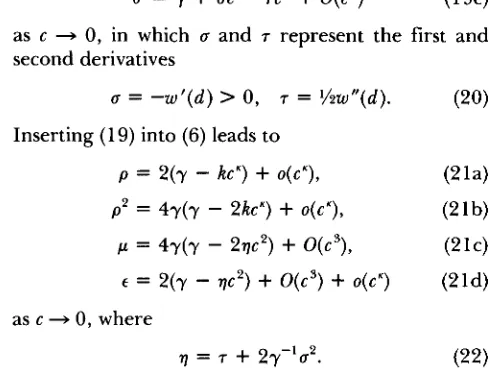
0, 7 = Y&"(d). (20)

Inserting (1 9) into (6) leads to

p = 2(y

-

kc")

+

o ( c K ) , ( 2 1 4

p 2 = 4y(y

-

2kc")

+

o ( c I ) , (2 lb)

p = 4y(y - 2712)

+

0 ( c S ) , ( 2 1 4

E = 2(y

-

qc2)

+

O ( c 3 )

+

o ( c K ) (21d)

as c + 0, where

r] = 7

+

2y"uZ. (22)

From (1 9a) and (19b) we see that a

>

/3 for suffi-

ciently small c. Table 3 and (2 1) inform us that as c --.,

0 with d fixed, either Case e or Case f applies, as

shown in Table 4. According to Table 4, if w ( z )

decreases rapidly near the optimum ( K

<

2), the sym-

metric equilibrium (Po) is globally stable for suffi-

ciently weak selection at the minor locus. This has the

important consequence that Po is globally stable with

arbitrarily weak selection, provided d / c is sufficiently

large. If w ( z ) decreases more slowly near the optimum

( K L 2), the existence of a stable internal equilibrium

depends on the major-locus effect ( d ) and details of

the fitness function.

We can obtain more insight for K 2: 2 by studying

the limits d + 0 and d -+ 00 (after taking the limit c +

0). From (18), (20), and (22), we find

r](d)

-

! / & K ( ~ K l ) d K - 2 (23)

as d + 0. Hence, Table 4 reveals that Case e holds

for sufficiently small d . For most simple fitness func-

tions, w " ( z )

>

0 for sufficiently large z, and w ' ( z ) ,

w " ( z ) 3 0 as z

*

00. Under these conditions,

r](d) 4

O+ as d + 00, whence Table 4 implies for sufficiently

large d that Cases f and e apply for K = 2 and K

>

2,

respectively. Thus, if K 2 2, the existence of a stable

internal equilibrium requires strong selection at the

major locus. These observations further support the conclusion of the previous paragraph that rapid de-

crease of w ( ~ ) near the origin enhances the opportu-

nity for stable polymorphism.

Weak selection at both loci: We have already

proved that Case f applies as d + 03 with c fixed. By

Table 4, if K C 2 in (IS), then Case f also applies as

c + 0 with d fixed. We conclude that if K

<

2, the

boundary curves E = p and p = p4 must emanate from

the origin. Therefore, we assume that K

<

2 and seek

their slopes at the origin. These will yield the classification of the convergence patterns in the weak-selec-

tion limit (0 C c 5 d + 0) for fitness functions that

decrease rapidly near the optimum ( K

<

2).

We put

[ = d / c (24)

and assume

6

remains bounded as c + 0. Appealing

to ( 3 ) and (18), we derive

a = kc"([

-

1)"

+

0 ( c X ) , (2 5a)

/3

= kc"

+

o(c"), (2 5b)

y = kc"E"

+

o ( c K ) , ( 2 5 4

6 = kc"([

+

1)"

+

o ( c K ) ( 2 5 4

as c + 0 with bounded. In the limit c + 0, we obtain

the slopes

&

and

&,

of E = p and p = p2, respectively,

at the origin.

Consider first E = p . Inserting (25) into (6) and

letting c "$0 lead to

(Xo

+

2)(Xg

-

mg) = 2([:

-

1)(Xg

+

ma), (26a)

where

X0 = (&

+

1)"

+

(&

-

1)" - 2, (26b)

mo = (&

+

1)" - (&

-

1)". (264

By (8c) and (24), E C 0 C p if

4

C 2, so we investigate

(26) only in [2, 00); assertions of uniqueness refer only

to this interval. If K = 1, it is easy to see that (26) has

the unique root

&

= 2

+

&.

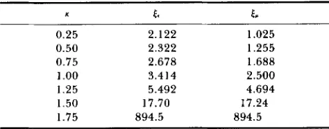
We offer some numerical

examples in Table 5; the roots appear to be unique.

Intuition and Table 5 suggest that

& +

2+ as K +

O+. This observation enables us to approximate [e for

K

<<

1. We substitute

tc

= 2

+

Oc (27)

into (26) and expand as K + O+ and O, + O+; we find

= [%(In 2)(ln 3)] K

+

O(O:

+

KO,)

(7)

TABLE 5

The slopes of the boundary curves e = p and p

=

pp at the origin

X €6 E,

0.25 2.122 1.025

0.50 2.322 1.255

0.75 2.678 1.688

I

.oo

3.414 2.500

1.25 5.492 4.694

1.50 17.70 17.24

1.75 894.5 894.5

The parameters are defined in (6), (18). and (24).

as K + 0. T h e constant in brackets is about 0.3808.

Equation 28 is fairly accurate even for K as large as

0.25, in which case the relative error is 1.2%.

Intuition and Table 5 also indicate that

El

+ w as

K + 2-. Therefore, we set

ve = l/Ef (29)

and rewrite (26) as

(X,

+

2v:)(X:

-

m:) = 2(1

-

ut)@:

+

my), (30a)

where

X1 = ( 1

+

v ~)"

+

( 1

-

Y~)"

-

2 ~ : , (30b)

r n l = ( 1

+

v,)"

-

( 1

-

u,)". ( 3 0 4

Expanding (30) as u, + 0, we deduce

u: = 8"

+

O($) = K'[l

+

O(Y:)], (31a)

where

s = 2

-

K ,

e

= 1/2K(3K

+

1). (31b)

From (3 1 a) we get

E.

= P [ i

+

0 ( ~ - ~ , 5 7 ]

= P [ i

+

~ ( ~ - ~ e - ~ / ~ ) ]

(32)

as s + O+. This approximation has an error of 3.9%

for K = 1.50, but only about 0.01% for K = 1.75. T h e

expansion

e l / 5 = e-13/1471/s

11 +

%)I

(33)

exhibits the extremely rapid divergence of

&

as s -+

0.

We turn now to c~ = p2. Substituting (6a) into (6c),

we have

p = (36

-

a)(3a

-

6). (34)

Consequently, in the limit c + 0, (6b), (25), and (34)

yield

[3(&

+

1)"

-

e,

-

1 ~ 1 [ 3 ( ~ ,

-

1)"

-

(E,

+

V I

(35)

= 4(&

-

1)2.

Since d 2 c, we examine (35) only in [ 1, 00); all

TABLE 6

Classification of the convergence patterns for weak selection with 0 < K < 2

Condition Case

1 I < rnin(2,t,,) d rnin(2,(,) < 5 max(2.6) b or e

rnax(2.W < I

-=

C

I > '5 f

The parameters are defined in (18). (24), and Table 5. In the second line, Case b applies if I, < 2 and Case e does if

[,

> 2. The inequality I, < 2 holds if and only if K 5 0.8690.

assertions of uniqueness are confined to this interval. If K = 1 , we can see easily that (35) has the unique

solution

E,

= 5/2. T h e roots in Table 5 appear to be

unique. Observe that, as the case maps in the next

section suggest,

4. >

4,

in Table 5.

Evidently,

&,

+ 1 + as K + O+. We insert

4,

= 1

+

w, (36)

into (35) and rearrange it in the form

3w;

-

(2

+

w,)" = 4[(1

+

w,)"

-

11'

3(2

+

w,)"

-

w; * (37)

Since the denominator on the right side of (37) ex-

ceeds 2 for 0

<

w,

<

1 , therefore, as K + O+ and

w, + 0+, (37) becomes

3Wi

-

(2

+

Up)" =

o(K20:).

(38)

Hence,

31/"w, = (2

+

w,>[ 1 O(KW;)], (39)

which has the solution

0

as K + 0. Equation 40 is accurate even if K is as large

as 0.25: then the error is 0.44%. According to (40),

w, + 0 extremely rapidly as K + 0; e.g., w,

=

3.387 X

Manifestly, E, + 00 as K + 2-. Setting u, = 1/[, as

in (29) and expanding (35) as V , + 0, we find that up

satisfies (3 1). We conclude that

6,

is also given by (32).

Thus,

&/&,

+ 1 as K + 2. Equation 32 is fairly accurate

even for K as small as 1.50: then the error is 1.3%; if

K = 1.75, the error is only about 0.01%.

Invoking Table 3, we obtain the classification of the

convergence patterns in Table 6. In the second line, Case b applies if

5,

<

2 and Case e does if E,,

>

2. By

setting

6,

= 2 and solving for K in (35), we deduce that

E,

<

2 if and only if K 5 0.8690. Tables 5 and 6

demonstrate that, in the weak-selection limit, the

(8)

T. Nagylaki

optimum, the less stringent are the conditions for

locally

( E

>

E,)

and globally ( E

>

&) stable two-locus

polymorphism. If the decrease is fairly rapid ( K 5

0.25), only a very slight disparity between the effects

of the major and minor loci is required for local

stability. 'This disparity must be substantial, however,

for K 2 1, and it increases extremely fast as K 4 2.

T h e condition for global stability is more restrictive:

4 >

2

is necessary but not sufficient.

Strong selection at both loci: In this subsection,

we assume that w ( z ) 4 0 as z 4 CQ and investigate

the boundary curves E = p and p = p2 in the limit d 2

As c + w , (3) yields

P,

y, 6 + 1, whence (6b) gives

p + 0. Therefore, E 4 0 along E = p and p + 0 along

p = p 2 . Since d = 2c and E = 0 are equivalent by (8c),

we expect E = p to be asymptotic to d = 2c.

On account of (34), p = 0 is equivalent to 6 = 3a.

Thus, we expect p = p2 to be asymptotic to

c + w.

1 - w(d

+

C) = 3[1

-

w(d

-

c)]. (41)

As c + w, the left side of (41) converges to one, so

w(d

-

C) +

*A.

(42)

Consequently, we expect p = p2 to be asymptotic to

the line

d = c

+

r , w ( r ) = %. (43)

Since w ( z ) decreases monotonically from 1 to 0 as z

increases from 0 to w, there exists a unique constant

r in (0, 00).

EXAMPLES

Here we illustrate the results of the last two sections by classifying the convergence patterns for some specific fitness functions.

The quadratic fitness function: Scaling c and d in

terms of the selection intensity allows us to take

w ( z ) = 1 - 2 , 0 I z 5 1, (44)

without loss of generality. From (3), (6), and (44), we

find

p = 2(d2

-

c'), ( 4 5 4

p = 4(d4

-

14c2d'

+

c4), (45W

6 = 2(d2

+

c') d 2

-

4c2

d 2

+

4 c 2 '

Trivial manipulation of (45) yields E

<

p and p

<

p2,

so Table 3 gives Case d for d 5 2c and Case e for d

>

2c. Thus, in agreement with WRIGHT (1935), at most

one locus can segregate stably. This was discussed further in the last section.

The triangular fitness function: On the appropri-

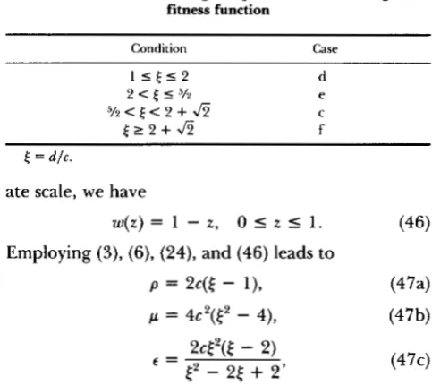
TABLE 7

Classification of the convergence patterns for the triangular fitness function

Condition Case

1 5 [ 5 2 d

2 e f 5 5/2 e

5 1 ~ < [ < 2 + f i C

[ r 2 + & f

[ = d / c .

ate scale, we have

w ( z ) = 1 - z, 0 I z I 1. (46)

Employing (3), (6), (24), and (46) leads to

2cE2(E -

2)

E'

-

2E

+

2' E =

whence we see easily that E

>

p and p

>

p2 are

equivalent to

E

>

2

+ &

and

>

5/2, in agreement

with (26) and (35), respectively. Table 3 then yields Table

7,

excluding [ = 5/2 and

4

= 2

+

&.

T o classify

these two values, note first that g = 4 c

>

0, so the line of equilibria (13) does not exist. If E = 5 / ~ , then E

<

p ,

so the edge equilibria P, are stable by Theorem 2, and

hence PO is unstable. Therefore, Figure l e applies. If

E

= 2

+

&,

then p

>

p2, so Po is stable by Theorem

3, and hence the pair P, is unstable. Therefore, Figure

1 f applies.

T h e fitness function (46) generalizes that of GALE

and KEARSEY (1968) to arbitrary selection intensity

(their 1

+

k

is our E). We have found that there exists

a stable internal equilibrium if and only if the ratio of

the effects of the major and minor loci, E , exceeds 5/2;

the stability is global if and only if

E

2 2

+

a.

GALE

and KEARSEY (1968) incorporate linkage and find

numerically that, for a fixed, large selection coeffi-

cient, the critical value of increases from about 1.2

to about 2.0 as the recombination frequency increases

from 0.05 to 0.50. Since all their examples exhibit

considerable linkage disequilibrium, it is not surpris-

ing that their critical values do not approach 5/2, as

they would for weak selection. By neglecting linkage

disequilibrium, we have obtained critical values that

are independent of the selection intensity and higher

than the exact ones.

The Gaussian fitness function: Our most impor-

tant example is

w ( z ) = e-". (48)

Let us prove first that g

>

0; by Proposition 1, this

implies that Case a does not occur. Appealing to (3),

(6a), (6b), (7b), and (48), we obtain

(9)

Stabilizing Selection

3

2 d

1.30

1

0

1

2

3 c

FIGURE 2.-The case map for the Gaussian fitness function (31). T h e boldface letters refer to the cases in Table 3 and Figure 1 . T h e coordinate c designates the effect of the minor locus; d is that of the major one. T h e o t h e r parameters are defined in Equations 3 and 6.

where

= e-(d+cji + e-(d-C)2

= 2e-C2-d2 cosh(2cd)

>

2e-"2_d2. ₍₅₀₎

Substituting (50) into (49a) produces

g

>

4(1 - e-")(l

-

e-d2)

>

0 . (51)

Second, from (1 8), (20), (22), and (48), we find that

7

<

k

if and only if

-

2veu

-

6v

-

1

>

0, (52)

where v = d2. It is easy to see that the equation

associated with the inequality (52) has a unique positive root. Evaluating it numerically, we infer from

Table 4 (since K =

2

here) that, as c + 0 , Case e applies

for d

<

do

=

1.30 1, whereas Case f applies for d

>

do.

Third, the asymptotic parameter in (43) is r =

(In 3/2)1/2

=

0.6368.

T h e case map exhibited in Figure

2

agrees with the

above analytic results. As expected, it shows that for

weak selection one may use the quadratic fitness func-

tion (44). T h e symmetric equilibrium ( P O ) is stable

above the curve = p2; the unsymmetric equilibria

(P,) are unstable when they exist (Cases b and c), and

then the stability of PO is not global. T h e most impor-

tant conclusion from Figure 2 is that, even for arbitrarily weak selection at the minor locus, strong selec-

tion at the major locus (d

>

do) is necessary for the

maintenance of genetic variability at both loci. T h e case map for

w ( z ) = 1/(1

+

z') (53)

3

2 d

1

0

1

2

3 c

FIGURE 3.-The case map for the double-exponential fitness function (37).

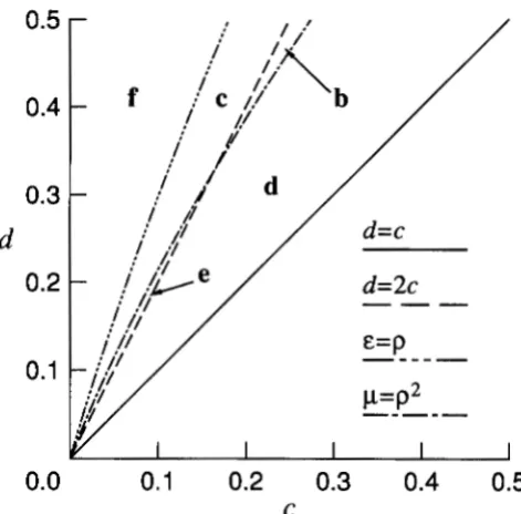
0.3 d

0.2

0.1

V I I I I I

0.0

0.1

0.2

0.3

0.4

0.5

C

FIGURE 4.-The case map for the double-exponential fitness function (37) near the origin.

is qualitatively identical to Figure 2. Direct algebra establishes that g

>

0. Now do

= 1.094 and

r = l / &

=

0.707 1.

The doubleexponential fitness function: For

w ( z ) = e-*, z 2 0 , (54)

by Proposition 1, convexity implies that g

>

0 and

thus excludes Case a. Since K = 1

<

2, Table 4 tells us

that Case f applies if c is sufficiently small. In (43), we

(10)

displays these features. Near the optimum

(IzI

<<

l), (46) approximates (54). Therefore, as expected and

shown in Figure 4, for weak selection ( d

<<

1) the case

map for (54) agrees with Table 7. Thus, the discussion

below (47) is pertinent here.

Slow decrease near the optimum: In Figure 5, we

exhibit the case map for

w ( z ) = e - L 4 . (55)

Here, K = 4

>

2.

Although Figure 5 shows that Case

a does not occur, a Taylor series establishes that g

<

0 if d is sufficiently small. Thus, the conditions in Proposition 1 are not necessary. It is not difficult to

prove, however, that 9

>

0. Hence, in agreement with

Figure 5, in which the boundary curves are asymptotic

to, but do not reach, the ordinate, Table 4 demon-

strates that Case e applies as c + 0. Figure 5 exempli-

fies the fact that if w ( z ) decreases slowly near the

optimum, then strong selection (here, d 5 1.7 19; the

minimum occurs at c

=

0.4287) is required for stable

polymorphism at both loci. Furthermore, if selection is very weak at the minor locus (c

<<

l), then it must be very strong at the major locus (d

>>

1).

The case map is similar for

w ( z ) = 1/(1

+

z4), ( 5 6 )

except that the rate of convergence of the boundary curves to their asymptotes is much slower. Again, one

can prove that 9

>

0, thereby confirming analytically

the most interesting feature of the case map.

A n example with Case a: T h e attentive reader may have noticed that Case a (the only one with stable unsymmetric equilibria) occurs neither in any of the

3

2 d

1

0

1

2

3

C

FIGURE 5.-The case map for w ( z ) = C 4 .T h e boundary curves

are asymptotic to, but do not reach, the ordinate.

limits in the previous section nor in any of the above

examples. In fact, despite an extensive numerical

search, no smooth fitness function for which Case a occurs has been found. T h e fitness function

0 5 z 5 1,

w ( z ) =

(bsz")" ( 5 7 4

?%=O

= T i -

, z > l ,

b 3 = 6 2 - b l , z * = z - 1 (57W

d

0

1

2

3

4

C

FIGURE 6.-The case map for the fitness function (57). T h e boundary curves approach the ordinate very closely, but d o not touch it.

d

0

1

2

C

(11)

has exactly three continuous derivatives if bl # b2.

Choosing bl = 0.1 and b2 = 6.0, we obtain the case

map in Figures 6 and

7,

of which Case a occupies a

small region. Note that the relative rate of decrease

of w ( z ) is much greater for z

>

1 than for 0

<

z 5 1. Although the boundary curves approach the ordinate

very closely, by Table 4 (since K = 1 here) they cannot

touch it for d

>

0.

DISCUSSION

Here we recapitulate our main results and discuss extensions and further applications. Our sole approximation was to neglect linkage disequilibrium. There- fore, our results are most accurate for weak selection.

As explained below (2), we expect the inclusion of

linkage disequilibrium to relax the conditions for the existence of stable two-locus polymorphism without changing them qualitatively.

Our two-locus model of stabilizing selection is iden-

tical to the symmetric viability model in Table 2, with

the restriction (4) on the selection coefficients. In

addition to the four vertex equilibria PI and Pp, given

by (9), the two edge equilibria P,, given by (lo), and

the symmetric equilibrium Po: ( V 2 , %), there may be

(generically) two unsymmetric equilibria P*, as speci-

fied in Theorem 1. Theorems 2 and 3 give conditions

for the stability of P, and Po. A complete classification

of the six possible global convergence patterns is presented in Table 3 and Figure 1. T h e unsymmetric equilibria are stable only in Case a, and, as discussed at the end of the last section, this does not seem to

occur for most simple, smooth fitness functions w ( z ) .

If selection at the major locus is sufficiently strong,

Case f applies, i e . , the symmetric polymorphism Po

(where the genetic variance is maximal) is globally

stable. As shown in Table 4, if w ( z ) decreases rapidly

near the optimum [ K

<

2 in (1 S)], Po is globally stable

for sufficiently weak selection at the minor locus.

Tables 4, 5 , and 6 and Equations 26, 28, 32, 35, and

40 reveal that, at least for weak selection at the minor

locus, the more rapid the decrease of w ( z ) near the

optimum, the greater is the opportunity for stable

polymorphism. For weak selection at both loci, if this

decrease is fairly rapid ( K 5 0.25), even a very slight

disparity between the effects of the major and minor

loci produces local stability of Po. This disparity must

be substantial, however, for K k 1, and it increases

extremely fast as K -+ 2. T h e condition for global

stability of Po is more stringent: it is necessary, but

not sufficient, that the disparity d / c

>

2.

Figure 2 demonstrates that for the Gaussian fitness

function (which has K = 2), strong selection at the

major locus ( d k 1.30 1) is necessary for the mainte-

nance of genetic variability at both loci. This conclusion holds for all fitness functions that are smooth at

TABLE 8

Classification of the convergence patterns for GIMELFARB’S (1986) pleiotropic model

Case Condition

A Sz 5 SI/(^

+

S I )

B $,/(?I

+

SI) < S2 < %SI

C %SI 5 S p 5 SI

The parameters are defined in (58); 0 < S P 5 s I 5 %. Figure 8 shows the global convergence patterns in the three cases.

p24

FIGURE 8.-The three possible convergence patterns for GIMEL- FARB’S (1986) pleiotropic model. The coordinates are the gene frequencies at the two loci.

the optimum. As Figure 5 exemplifies, if w ( z ) de-

creases slowly near the optimum ( K

>

2) and selection

is weak at the minor locus, then selection must be very strong at the major locus.

Despite the biological simplicity of the model

(12)

246

1/2 at each locus) for any symmetric, monotone de-

creasing fitness function. Instability for two loci sug- gests, but does not prove, multilocus instability.

Our results and approach have other, closely related

applications. GIMELFARB (1986) noted that his two-

locus model of pleiotropy for two quantitative char-

acters is a special case of the symmetric viability model:

(Y = 4 S p , 6 = 4 S 1 , ( 5 8 4

p

= y = s1

+

sp

-

SIS2, (58W

where SI and sp, 0

<

sp 5 SI 5 %, denote the intensities

of quadratic stabilizing selection on the two charac-

ters. Since

p

= y here, this model is much easier to

analyze than the general one in Table

2,

Nevertheless,

slight modifications of our results are required be-

cause y

<

a is possible, so that (4) may not hold. T h e

four edge equilibria

x = TV2, y = +(SI

-

sp)/(sl

+

sp

+

sIsp), (59a)

X = +(SI

-

s~)/(sI

+

s:,

+

sIs~), J = T1/2 (59b) exist if and only if S l / ( 3

+

SI)

<

sp 5 SI. T h e pair of

unsymmetric internal equilibria

X = +[(SI

-

3 ~ p ) / ( 4 ~ 1 ~ p ) ] ” ’ , J = --X (60)

exists if and only if s1/(3

+

SI)

<

sp

<

%SI.

In Table 8, we classify the three possible conver-

gence patterns exhibited in Figure 8. If selection on

one character is considerably stronger than on the

other, Case A applies and both loci are ultimately

fixed. In a narrow range of appreciable disparity

between the two selection intensities, Case B applies and the gene frequencies converge to one of the two unsymmetric polymorphisms. If the disparity is at most a factor of three, there is global convergence to the symmetric polymorphism (Case C).

These approximate analytic results agree com-

pletely with GIMELFARB’S (1 986) numerical examples.

For various combinations of sl and sp, he computed

for the exact model the maximum value of the recom-

bination frequency, T * , for which a stable symmetric

polymorphism exists. He found that r*

<

?h for S I / S ~

2 4 and r* = Y2 for sI/sp 5 3; he did not study the unsymmetric equilibria.

A . GIMELFARB’S (unpublished manuscript) two-locus

epistatic model is invariant under the interchange of

the gene frequencies at the two loci ($11 t.)f ~ ) , unlike

the symmetric viability model, which is invariant under the simultaneous interchange of each gene frequency and its complement

(PI

t,q l and $I2 t.)q 2 ) .

Therefore, this model requires a new analysis.

1 an1 grateful to R. BAHADUR, A. GIMELFARB, R. LANDE, and B. MERRIMAN for helpful discussions, G. WAGNER for perceptive com- ments on the manuscript, and B. MERRIMAN for highly professional numerical calculations. This work was supported by National Sci- ence Foundation grant BSR-8512844.

LITERATURE CITED

APOSTOL, T. M., 1974 Mathematical Analysis, Ed. 2. Addison- Wesley, Reading, Mass.

BARTON, N. H., 1986 The maintenance of polygenic variation through a balance between mutation and stabilizing selection. Genet. Res. 47: 209-216.

BARTON, N. H., and M. TURELLI, 1987 Adaptive landscapes, genetic distance and the evolution of quantitative characters. Genet. Res. 4 9 157-173.

BAUM, I,. E., and J. A. EAGON, 1967 An inequality with applications to statistical estimation for probabilistic functions of a Markov process and to a model in ecology. Bull. Am. Math. SOC. 73: 360-363.

BODMER, W. F., and J. FELSENSTEIN, 1967 Linkage and selection: theoretical analysis of the deterministic two locus random mating model. Genetics 57: 237-265.

BULMER, M. G., 1971 The stability of equilibria under selection. Heredity 27: 157-162.

BULMER, M. G., 1973 The maintenance of the genetic variability of polygenic characters by heterozygous advantage. Genet. Res.

22: 9-12.

BURGER, R., 1986 On the maintenance of genetic variation: Global analysis of Kimura’s continuum-of-alleles model. J. Math. Biol. 24: 341-351.

BURGER, R., 1988 Mutation-selection balance and continuum of alleles models. Math. Biosci. 91: 67-83.

BURGER, R., 1989 Linkage and the maintenance of heritable variation by mutation-selection balance. Genetics 121: 175-

184.

ENDLER, J. A,, 1986 Natural Selection in the Wild. Princeton Uni-

FISHER, R. A,, 1930 The Genetical Theory of Natural Selection.

GALE, J. S., and M . J. KEARSEY, 1968 Stable equilibria under stabilising selection in the absence of dominance. Heredity 23:

GILLESPIE, J. H., 1984 Pleiotropic overdominance and the maintenance of genetic variation in polygenic characters. Genetics

107: 321-330.

GIMELFARB, A,, 1986 Additive variation maintained under stabilizing selection: a two-locus model of pleiotropy for two quantitative characters. Genetics 112: 71 7-725.

HASTINGS, A,, 1985 Four simultaneously stable polymorphic equi-

HASTINGS, A,, 1987 Monotonic change of the mean phenotype in

KARLIN, S., and M. W. FELDMAN, 1970 Linkage and selection: two locus symmetric viability model. Theor. Popul. Biol. 1: 39- 71.

KEARSEY, M . J., and J. S. GALE, 1968 Stabilising selection in the absence of dominance: an additional note. Heredity 23: 617- 620.

KIMURA, M . , 1981 Possibility ofextensive neutral evolution under stabilizing selection with special reference to nonrandom usage of synonymous codons. Proc. Natl. Acad. Sci. USA 78: 5773- 5777.

KOJIMA, K.-I., 1959 Stable equilibria for the optimum model. Proc. Natl. Acad. Sci. USA 45: 989-993.

LEWONTIN, R. C., 1964 The interaction of selection and linkage.

MORAN, P. A. P., 1963 Balanced polymorphisms with unlinked

NAGYLAKI, T., 1976 T h e evolution of one- and two-locus systems.

NAGYLAKI, T., 1977a Selection in One- and Two-Locus Systems.

versity Press, Princeton, N.J.

Clarendon Press, Oxford.

553-561.

libria in two-locus two-allele models. Genetics 109: 255-26 1.

two-locus models. Genetics 117: 583-585.

11. Optimum models. Genetics 5 0 757-782.

loci. Aust. J. Biol. Sci. 16: 1-5.