© 2013, IJCSMC All Rights Reserved
190
Available Online atwww.ijcsmc.com
International Journal of Computer Science and Mobile Computing
A Monthly Journal of Computer Science and Information Technology
ISSN 2320–088X
IJCSMC, Vol. 2, Issue. 11, November 2013, pg.190 – 202
RESEARCH ARTICLE
Position Spatial Data by Eminence Preferences
SHAIKH ISULAL SULEMAN
1, M. YASEEN PASHA
2, K. SHARATH KUMAR
31
MTech CSE Student, Sphoorthy Engineering College, JNTU Hyderabad,
Hyderabad, Andhra Pradesh, India
2
Assistant Professor, Department of CSE, Sphoorthy Engineering College,
Hyderabad, Andhra Pradesh, India
3
Head of the Department of CSE & IT, Sphoorthy Engineering College,
Hyderabad, Andhra Pradesh, India
Abstract—A spatial preference query ranks objects based on the qualities of features in their spatial neighborhood. For example,using a real estate agency database of flats for lease, a customer may want to rank the flats with respect to the appropriateness of their location, defined after aggregating the qualities of other features (e.g., restaurants, cafes, hospital, market, etc.) within their spatial neighborhood. Such a neighborhood concept can be specified by the user via different functions. It can be an explicit circular region within a given distance from the flat. Another intuitive definition is to consider the whole spatial domain and assign higher weights to the features based on their proximity to the flat. In this paper, we formally define spatial preference queries and propose appropriate indexing techniques and search algorithms for them. Extensively evaluation of our methods on both real and synthetic data reveals that an optimized branch-and-bound solution is efficient and robust with respect to different parameters.
Keywords:—H.2.4.h Query processing; H.2.4.k Spatial databases
1 INTRODUCTION
Spatial database systems manage large collections of geographic entities, which apart from spatial attributes contain non-spatial information (e.g., name, size, type, price, etc.). In this paper, we study an interesting type of preference queries, which select the best spatial location with respect to the Eminence of facilities in its spatial neighborhood.
Given a set D of interesting objects (e.g., candidate locations), a top-k spatial preference query retrieves the k objects in D with the highest scores. The score of an object is defined by the Eminence of features (e.g., facilities or services) in its spatial neighborhood. As a motivating example, consider a real estate agency office that holds a database with available flats for lease. Here “feature” refers to a class of objects in a spatial map such as specific facilities or services. A customer may want to rank the contents of this database with respect to the Eminence of their locations, quantized by aggregating non-spatial characteristics of other features (e.g., restaurants, cafes, hospital, market, etc.) in the spatial neighborhood of the flat (defined by a spatial range around it). Eminence may be subjective and query-parametric. For example, a user may define Eminence with respect to non-spatial attributes of restaurants around it (e.g., whether they serve seafood, price range, etc.).
© 2013, IJCSMC All Rights Reserved
191
(a) range score, =0.2 km (b) influence score, =0.2 km Fig. 1. Examples of top-k spatial preference queries
to find a hotel p that is close to a high-Eminence restaurant and a high-Eminence cafe. Figure 1a illustrates the locations of an object dataset D (hotels) in white, and two feature datasets: the set F1 (restaurants) in gray, and the set F2 (cafes) in black. Feature points are labeled by Eminence values that can be
obtained from rating providers (e.g., http://www.zagat.com/). For the ease of discussion, the qualities are normalized to values in [0. 1]. The score (p) of a hotel p is defined in terms of: (i) the maximum Eminence for each feature in the neighborhood region of p, and (ii) the aggregation of those qualities.
A simple score instance, called the range score, binds the neighborhood region to a circular region at p with radius (shown as a circle), and the aggregate function to SUM. For instance, the maximum Eminence of gray and black points within the circle of p1 are 0.9 and 0.6 respectively, so the score of p1 is (p1) =
0.9 + 0.6 = 1.5. Similarly, we obtain (p2) = 1.0+0.1 = 1.1 and (p3) = 0.7+0.7 = 1.4. Hence, the hotel p1 is returned as the top result.
In fact, the semantics of the aggregate function is relevant to the user’s query. The SUM function attempts to balance the overall qualities of all features. For the MIN function, the top result becomes p3, with the score (p3) = min{0.7. 0.7} = 0.7. It ensures that the top result has reasonably high qualities in all
features. For the MAX function, the top result is p2, with (p2) = max{1.0. 0.1} = 1.0. It is used to optimize the Eminence in a particular feature, but not
necessarily all of them.
The neighborhood region in the above spatial preference query can also be defined by other score functions. A meaningful score function is the influence score (see Section 4). As opposed to the crisp radius constraint in the range score, the influence score smoothens the effect of and assigns higher weights to cafes that are closer to the hotel. Figure 1b shows a hotel p5 and three cafes s1. s2.s3 (with their Eminence values). The circles have their radii as multiples of
.Now, the score of a cafe si is computed by multiplying its Eminence with the weight 2 j, where j is the order of the smallest circle containing si. For example,
the scores of s1, s2, and s3 are 0.3/21 = 0.15, 0.9/22 = 0.225, and 1.0/23 = 0.125 respectively. The influence score of p5 is taken as the highest value (0.225).
Traditionally, there are two basic ways for position objects: (i) spatial position, which orders the objects according to their distance from a reference point, and (ii) non-spatial position, which orders the objects by an aggregate function on their non-spatial values. Our top-k spatial preference query integrates these two types of position in an intuitive way. As indicated by our examples, this new query has a wide range of applications in service recommendation and decision support systems.
To our knowledge, there is no existing efficient solution for processing the top-k spatial preference query. A brute-force approach (to be elaborated in Section 3.2) for evaluating it is to compute the scores of all objects in D and select the top-k ones. This method, however, is expected to be very expensive for large input datasets. In this paper, we propose alternative techniques that aim at minimizing the I/O accesses to the object and feature datasets, while being also computationally efficient. Our techniques apply on spatial-partitioning access methods and compute upper score bounds for the objects indexed by them, which are used to effectively prune the search space. Specifically, we contribute the branch-and-bound algorithm (BB) and the feature join algorithm (FJ) for efficiently processing the top-k spatial preference query.
Furthermore, this paper studies three relevant extensions that have not been investigated in our preliminary work. The first extension (Section 3.4) is an optimized version of BB that exploits a more efficient technique for computing the scores of the objects. The second extension (Section 3.6) studies adaptations of the proposed algorithms for aggregate functions other than SUM, e.g., the functions MIN and MAX. The third extension (Section 4) develops solutions for the top-k spatial preference query based on the influence score.
The rest of this paper is structured as follows. Section 2 provides background on basic and advanced queries on spatial databases, as well as top-k query evaluation in relational databases. Section 3 defines the top-k spatial preference query and presents our solutions. Section 4 studies the query extension for the influence score. In Section 5, our query algorithms are experimentally evaluated with real and synthetic data. Finally, Section 6 concludes the paper with future research directions.2
2 BACKGROUND
Object position is a popular retrieval task in various applications. In relational databases, we rank tuples using an aggregate score function on their attribute values. For example, a real estate agency maintains a database that contains information of flats available for rent. A potential customer wishes to view the top-10 flats with the largest sizes and lowest prices. In this case, the score of each flat is expressed by the sum of two qualities: size and price, after normalization to the domain [0,1] (e.g., 1 means the largest size and the lowest price). In spatial databases, position is often associated to nearest neighbor (NN) retrieval. Given a query location, we are interested in retrieving the set of nearest objects to it that qualify a condition (e.g., restaurants). Assuming that the set of interesting objects is indexed by an R-tree, we can apply distance bounds and traverse the index in a branch-and-bound fashion to obtain the answer.
2.1 Spatial Query Evaluation on R-trees
The most popular spatial access method is the R-tree [3], which indexes minimum bounding rectangles (MBRs) of objects. Figure 2 shows a set D ={p1. : : : .
p8} of spatial objects (e.g., points) and an R-tree that indexes them. R-trees can efficiently process main spatial query types, including spatial range queries,
nearest neighbor queries, and spatial joins. Given a spatial region W , a spatial range query retrieves from D the objects that intersect W . For instance, consider a range query that asks for all objects within the shaded area in Figure 2. Starting from the root of the tree, the query is processed by recursively following entries, having MBRs that intersect the query region. For instance, e1 does not intersect the queryregion, thus the subtree pointed by e1 cannot contain any query
result. In contrast, e2 is followed by the algorithm and the points in the corresponding node are examined recursively to find the query result p7.
© 2013, IJCSMC All Rights Reserved
192
using the best-first (BF) algorithm of [4], provided that D is indexed by an R-tree. A min-heap H which organizes R-tree entries based on the (minimum) distance of their MBRs to q is initialized with the root entries. In order to find the NN of q in Figure 2, BF first inserts to H entries e1, e2, e3, and their distances
to q. Then the nearest entry e2 is retrieved from H and objects p1. p7.p8 are inserted to H. The next nearest entry in H is p7, which is the nearest neighbor of q. In
terms of I/O, the BF algorithm is shown to be no worse than any NN algorithm on the same R-tree [4].
The aggregate R-tree (aR-tree) [10] is a variant of the R-tree, where each non-leaf entry augments an aggregate measure for some attribute value (measure) of all points in its subtree. As an example, the tree shown in Figure 2 can be upgraded to a MAX aR-tree over the point set, if entries e1, e2,e3 contain the
maximum measure values of sets { p2, p3}{p1, p8, p7},{p4, p5, p6}, respectively. Assume that the measure values of p4, p5, p6are 0.2, 0.1, 0.4, respectively. In this
case, the aggregate measure augmented in e3 would be max{0.2, 0.1, 0.4} = 0.4. In this paper, we employ MAX aR-trees for indexing the feature datasets (e.g.,
restaurants), in order to accelerate the processing of top-k spatial preference queries.
Given a feature dataset F and a multi-dimensional region R, the range top-k query selects the tuples (from F) within ythe region R and returns only those with the k highest qualities. Hong et al. [11] indexed the dataset bya MAX aR-tree and developed an efficient tree traversal algorithm to answer the query. Instead of finding the best k qualities from F in a specified region, our (rangescore) query considers multiple spatial regions based on the points from the object dataset D, and attempts to find out the best k regions (based on scores derived from multiple feature datasets Fc).
Fig. 2. Spatial queries on R-trees
2.2 Characteristic based Spatial Queries
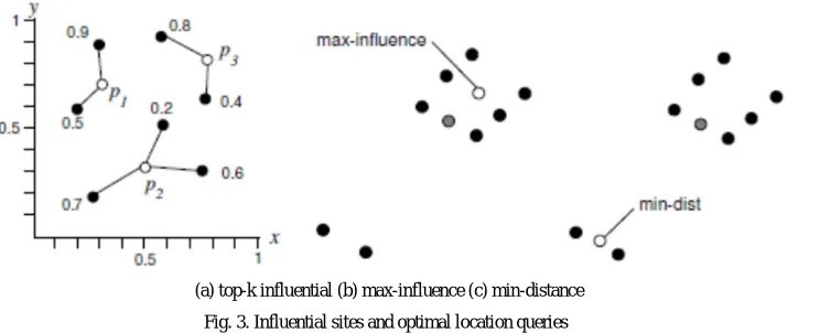
Xia et al. [12] solved the problem of finding top-k sites (e.g., restaurants) based on their influence on featurepoints . As an example, Figure 3a shows a set of sites (white points), a set of features (black points with weights), such that each line links a feature point to its nearest site. The influence of a site pi is defined
by the sum of weights of feature points having pi as their closest site. For instance, the score of p1 is 0.9+0.5=1.4. Similarly, the scores of p2 and p3 are 1.5 and
1.2 respectively. Hence, p2 is returned as the top-1 influential site.
Related to top-k influential sites query are the optimal location queries studied in . The goal is to find the location in space . Assume that all feature points have the same Eminence. The maximum influence optimal location query [13] finds the location (to insert to the existing set of sites with the maximum influence (as defined in [12]), whereas the minimum distance optimal location query [14] searches for the location that minimizes the average distance from each feature point to its nearest site. The optimal locations for both queries are marked as white points in Figures 3b,c respectively.
(a) top-k influential (b) max-influence (c) min-distance Fig. 3. Influential sites and optimal location queries
The techniques proposed in [12], [13], [14] are specific to the particular query types described above and cannot be extended for our top-k spatial preference queries. Also, they deal with a single feature dataset whereas our queries consider multiple feature datasets.
Recently, novel spatial queries and joins [15], [16], [17], [18] have been proposed for various spatial decision support problems. However, they do not utilize non-spatial qualities of facilities to define the score of a location. Finally, [19], [20] studied the evaluation of textual location-based queries on spatial objects.
3
Spatial Predilection
Section 3.1 formally defines the top-k spatial preference query problem and describes the index structures for the datasets. Section 3.2 studies two baseline algorithms for processing the query. Section 3.3 presents an efficient branch-and-bound algorithm for the query, and its further optimization is proposed in Section 3.4. Section 3.5 develops a specialized spatial join algorithm for evaluating the query. Finally, Section 3.6 extends the above algorithms for answering top-k spatial preference queries involving other aggregate functions.
3.1 Definitions and Index Structures
Let Fc be a feature dataset, in which each feature object s Fc is associated with a Eminencew( ) and a spatial point. We assume that the domain of w( )is the
© 2013, IJCSMC All Rights Reserved
193
Let D be an object dataset, where each object p € D is a spatial point. In other words, D is the set of interesting points (e.g, hotel locations) considered by the user.
Given an object dataset D and m feature datasetsF1,F2,.. Fm, the top-k spatial preference query retrieves the k points in D with the highest score. Here, the
score of an object point p € D is defined as:
where AGG is an aggregate function and t (p) is the (c-th) component score of p with respect to the neighborhood condition and the (c-th) feature dataset Fc.
We proceed to elaborate the aggregate function and the component score function. Typical examples of the aggregate function AGG are: SUM, MIN, MAX. We first focus on the case where AGG is SUM. In Section 3.6, we will discuss the generic scenario where AGG is an arbitrary monotone aggregate function.
An intuitive choice for the component score function c (p) is: the range score crng(p), taken as the maximum Eminence !(s) of points s 2 Fc that are within a
given parameter distance from p, or 0 if no such point exists.
Notation Meaning
e an entry in an R-tree
D the object dataset
m the number of feature datasets
Fc the c-th feature dataset
w(s) the Eminence of an point s in Fc
w(e) augmented Eminence of an aR-tree entry e of Fc
p an object point of D
c (p) the c-the component score of p
(p) the overall score of p
dist(p. s) Euclidean distance between two points p and s mindist(p. e) minimum distance between p and e maxdist(p. e) maximum distance between p and e
T (e) upper bound score of an R-tree entry e of D TABLE 1
List of Notations
3.2 Snooping
We first introduce a brute-force solution that computes the score of every point p D in order to obtain the query results. Then, we propose a group evaluation technique that computes the scores of multiple points concurrently.
Simple Snooping Algorithm
According to Section 3.1, the Eminence !(s) of any feature point s falls into the interval [0. 1]. Thus, for a point p D, where not all its component scores are known, its upper bound score +(p) is defined as:
It is guaranteed that the bound +(p) is greater than or equal to the actual score (p).
Algorithm 1 is a pseudo-code of the simple probing algorithm (SP), which retrieves the query results by computing the score of every object point. The algorithm uses two global variables: Wk is a min-heap for managing the top-k results and represents the top-k score so far (i.e., lowest score in Wk). Initially, the
algorithm is invoked at the root node of the object tree (i.e., N = D:root). The procedure is recursively applied (at Line 4) on tree nodes until a leaf node is accessed. When a leaf node is reached, the component scorec(e) (at Line 8) is computed by executing a range search on the feature tree Fc for range score
queries. Lines 6-8 describe an incremental computation technique, for reducing unnecessary component score computations. In particular, the point e is ignored as soon as its upper bound score +(e) (see Equation 3) cannot be greater than the best-k score . The variables Wk and are updated when the actual score (e)
is greater than .
Group Probing Algorithm.
Due to separate score computations for different objects, SP is inefficient for large object datasets. In view of this, we propose the group probing algorithm (GP), a variant of SP, that reduces I/O cost by computing scores of objects in the same leaf node of the R-tree concurrently. In GP, when a leaf node is visited, its points
Algorithm 1 Simple Probing Algorithm (SP)
algorithmSP(NodeN) 1: for each entrye N do
2: if Nis non-leaf then
3: read the child node NI pointed by e.
4: SP(NI ).
5: else
6: for c:=1 tom do
7: if +(e)> then . upper bound score
© 2013, IJCSMC All Rights Reserved
194
9: if (e)> then
10: update Wk (and ) by e.
are first stored in a set V and then their component scores are computed concurrently at a single traversal of the Fc tree. We now introduce some distance
notations for MBRs. Given a point p and an MBR e, the value mindist(p, e) (maxdist(p, e)) denotes the minimum (maximum) possible distance between p and any point in e. Similarly, given two MBRs ea and eb, the value mindist(ea,eb) (maxdist(ea,eb)) denotes the minimum (maximum) possible distance between any
point in ea and any point in eb.
Algorithm 2 shows the procedure for computing the c-th component score for a group of points. Consider a subset V of D for which we want to compute their crng(p) score at feature tree Fc. Initially, the procedure is called with N being the root node of Fc. If e is a non-leaf entry and its mindist from some point p
V is within the range , then the procedure is applied recursively on the child node of e, since the sub-tree of Fc rooted at e may contribute to the component
score of p. In case e is a leaf entry (i.e., a feature point), the scores of points in V are updated if they are within distance from e.
Algorithm 2 Group Range Score Algorithm
algorithmGroup Range(NodeN, SetV, Valuec, Value ) 1: for each entrye N do
2: if Nis non-leaf then
3: if ∃p V.mindist(p. e) then
4: read the child node NI pointed by e. 5: Group Range(NI ,V ,c, ). 6: else
7: for each p2Vsuch thatdist(p. e) do
8: c(p):=max{ c(p), (e)}.
3.3 Branch and Bound Algorithm
GP is still expensive as it examines all objects in D and computes their component scores. We now propose an algorithm that can significantly reduce the number of objects to be examined. The key idea is to compute, for non-leaf entries e in the object tree D, an upper bound T (e) of the score (p) for any point p in the subtree of e. If T (e)≤ , then we need not access the subtree of e, thus we can save numerous score computations.
Algorithm 3 is a pseudo-code of our branch and bound algorithm (BB), based on this idea. BB is called with N being the root node of D. If N is a non-leaf node,Lines 3-5 compute the scores T (e) for non-leaf entries e concurrently. Recall that T (e) is an upper bound score for any point in the subtree of e. The techniques for computing T (e) will be discussed shortly. Like Equation 3, with the component scores Tc(e) known so far, we can derive T+(e), an upper bound
of T (e). If T+(e)≤ , then the subtree of e cannot contain better results than those in Wk and it is removed from V . In order to obtain points with high scores
early, we sort the entries in descending order of T (e) before invoking the above procedure recursively on the child nodes pointed by the entries in V . If N is a leaf node, we compute the scores for all points of N concurrently and then update the set Wk of the top-k results. Since both Wk and are global variables, the
value of is updated during recursive call of BB.
Upper Bound Score Computation.
It remains to clarify how the (upper bound) scores Tc(e) of non-leaf entries (within the same node N) can be computed concurrently (at Line 4). Our goal is to
compute these upper bound scores such that
the bounds are computed with low I/O cost, and
the bounds are reasonably tight, in order to facilitate effective pruning.
To achieve this, we utilize only level-1 entries (i.e., lowest level non-leaf entries) in Fc for deriving upper bound scores because: (i) there are much fewer level-1
entries than leaf entries (i.e., points), and (ii) high level entries in Fc cannot provide tight bounds. In our experimental study, we will also verify the effectiveness
and the cost of using level-1 entries for upper bound score computation.
Algorithm 2 can be modified for the above upper bound computation task (where input V corresponds to a set of non-leaf entries), after changing Line 2 to check whether child nodes of N are above the leaf level.
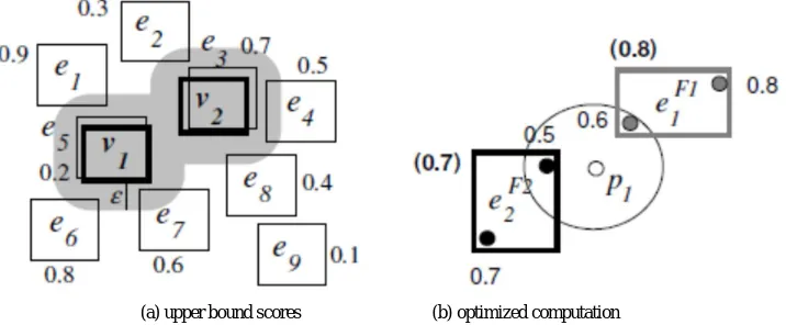
The following example illustrates how upper bound range scores are derived. In Figure 4a, v1 and v2 are non-leaf entries in the object tree D and the others
are level-1 entries in the feature tree Fc. For the entry v1, we firstdefine its Minkowski region [21] (i.e., gray region around v1), the area whose mindist from v1 is
within . Observe that only entries ei intersecting the Minkowski region of v1 can contribute to the score of some point in v1. Thus, the upper bound score Tc(v1)
is simply the maximum Eminence of entries e1, e5, e6, e7, i.e., 0.9. Similarly, Tc(v2) is computed as the maximum Eminence of entries e2, e3, e4, e8, i.e., 0.7.
© 2013, IJCSMC All Rights Reserved
195
(a) upper bound scores (b) optimized computation Fig. 4. Examples of deriving scores
The BB* Algorithm
Based on the above, we extend BB (Algorithm 3) to an optimized BB* algorithm as follows. First, Lines 11–13 of BB are replaced by a call to Algorithm 4, for computing the exact scores for object points in the set V . Second, Lines 3–5 of BB are replaced by a call to a modified Algorithm 4, for deriving the upper bound scores for non-leaf entries (in V ). Such a modified Algorithm 4 is obtained after replacing Line 18 by checking whether the node CN is a non-leaf node above the level-1.
3.5 Feature Join Algorithm
An alternative method for evaluating a top-k spatial preference query is to perform a multi-way spatial join [23] on the feature trees F1,F2,……Fm to obtain
combinations of feature points which can be in the neighborhood of some object from D. Spatial regions whichcorrespond to combinations of high scores are then examined, in order to find data objects in D having the corresponding feature combination in their neighborhood. In this section, we first introduce the concept of a combination, then discuss the conditions for a combination to be pruned, and finally elaborate the algorithm used to progressively identify the combinations that correspond to query results.
Fig. 5. Qualified combinations for the join
Tuple (f1,f2, … fm) is a combination if, for any ∁∈ [1, m], fc is an entry (either leaf or non-leaf) in the feature tree Fc. The score of the combination is defined
by:
For a non-leaf entry fc, !(fc) is the MAX of all feature qualities in its subtree (stored with fc, since Fc is an aR-tree). A combination disqualifies the query if:
When such a condition holds, it is impossible to have a point in D whose mindist from fi and fj are within respectively. The above validity check acts as a
multiway join condition that significantly reduces the number of combinations to be examined.
Figure 5a and 5b illustrate the condition for a non-leaf combination (A1, B2) and a leaf combination (a3. b4), respectively, to be a candidate combination for
the query.
Algorithm 5 Feature Join Algorithm (FJ) Wk:=new min-heap of size k (initially empty).
=0. . k-th score in Wk
algorithmFJ(TreeD,TreesF1,F2,……..Fm)
1: H:=new max-heap (combination score as the key). 2: insert(F1:root. F2:root..Fm:rooti into H.
3: while His not empty do
4: deheap hf1. f2..fmi from H.
© 2013, IJCSMC All Rights Reserved
196
6: for c:=1 tom do
7: read the child node Lc pointed by fc.
8: Find Result(D:root, L1.. Lm).
9: else
10: fc:=highest level entry among f1. f2..fm.
11: read the child node Nc pointed by fc.
12: for each entryec Nc do
13: insert hf1. f2..ec..fmi into H if its score is greater than and it qualifies the query. algorithmFind Result(NodeN, NodesL1.. Lm)
1: for each entrye N do
2: if Nis non-leaf then
3: compute T (e) by entries in L1.. Lm.
4: if T(e)> then
5: read the child node N0 pointed by e. 6: Find Result(N0 , L
1.. Lm).
7: else
8: compute (e) by entries in L1.. Lm.
9: update Wk (and ) by e (when necessary).
is inserted into H for further processing if its score is higher than and it qualifies the query. The loop (at Line 3) continues until H becomes empty.
3.6 Extension to Monotonic Aggregate Functions
We now extend our proposed solutions for processing the top-k spatial preference query defined by any mono-tonic aggregate function AGG. Examples of AGG include (but not limited to) the MIN and MAX functions.
Adaptation of incremental computation
Recall that the incremental computation technique is applied by algorithms SP, GP, and BB, for reducing I/O cost. Specifically, even if some component score
c(p) of a point p has not been computed yet, the upper bound score +(p) of p can be derived by Equation 3. Whenever +(p) drops below the best score found so
far , the point p can be discarded immediately without needing to compute the unknown component scores of p.
In fact, the algorithms SP, GP, and BB are directly applicable to any monotonic aggregate function AGG because Equation 3 can be generalized for AGG. Now, the upper bound score +(p) of p is defined as:
Due to the monotonicity property of AGG, the bound +(p) is guaranteed to be greater than or equal to the actual score (p). Adaptation of upper bound computation
The BB* and FJ algorithms compute the upper bound score of a non-leaf entry of the object tree D or a combination of entries from feature trees, by summing its upper bound component scores. Both BB* and FJ are applicable to any monotonic aggregate function AGG, with only the slight modifications discussed below. For BB*, we replace the summation operator by AGG, in Equation 4, and at Lines 14 and 26 of Algorithm 4. For FJ, we replace the summation by AGG, in Equation 5.
4 SWAY SCORE
4.1 Score Definition
The range score has a drawback that the parameter is not easy to set. Consider for instance the example of the range score rngin Figure 6a, where the white
points are object points in D, the gray points and black points are feature points in the feature sets F1 and F2 respectively. If is set to 0.2 (shown by circles), then
the object p2 has the score rng(p2) = 0:9 + 0:1 = 1:0 and it cannot be the best object (as rng (p1) = 1:2). Thishappens because a high-Eminence black feature is
barely outside the -range of p2. Had been slightly larger, that black feature would contribute to the score of p2, making it the best object.
© 2013, IJCSMC All Rights Reserved
197
4.2 Query Processing for SP, GP, BB, and BB*
We now examine the extensions of the SP, GP, BB, and BB* algorithms for top-k spatial preference queries defined by the influence score in Equation 8.
Incremental computation technique
Observe that the upper bound of is 1. Therefore, Equation 3 still holds for the influence score, and the incremental computation technique (see Section 3.2) can still be applied in SP, GP, and BB.
Exact score computation for a single object.
For the SP algorithm, we elaborate how to compute the score ) (see Equation 8) of an object p 2 D. This
is challenging because some feature s belongs to Fc outside the range of p may contribute to the score. Unlike the computation of the range score, we can no longer use the -range to restrict the search space. Given an object point p and an entry e from the feature tree of Fc, we define the upper bound function:
In case e is a leaf entry (i.e., a feature point s), we have . The following lemma shows that the value !inf (e; p) is an upper bound of winf (eI, p) for any entry e0 in the subtree of e.
Group computation and upper bound computation
Recall that, for the case of range scores, both the GP and BB algorithms apply the group computation technique (Algorithm 2) for concurrently computing the component score Tc(p) for every object point p in a given set V . Now, Algorithm 6 can be modified as follows to support concurrent computation of influence scores. Firstly, the parameter p is replaced by a set V of objects. Second, we initialize the value Tc(p) for each object p V at Line 3 and perform the score update for each p V at Line 13. Thirdly, the conditions at Lines 6 and 10 are checked whether they are satisfied by some object p V .
Optimized computation of scores in BB*.
Given an entry e (from a feature tree), we define the upper bound score of e using a set V of points as:
4.3 Query Processing for FJ
© 2013, IJCSMC All Rights Reserved
198
Algorithm 7 is the pseudo for computing the upper bound score for the combination (f1, f2,……, fm) of feature entries. The parameter represents the best score found so far (in FJ). The value Imax is used to control the number of iterations in the algorithm; its typical value is 20. At Line 1, we employ a max-heap H to organize its rectangles in descending order of their upper bound scores. Then, we insert the spatial domain rectangle into H. The loop at Line 4 continues while H is not empty and Imax> 0. After deheaping a rectangle r from H (Line 5), we partition it into four child rectangles. Each child rectangle r0 is inserted into H if its upper bound score is above . We then decrement Imax (at Line 10). At the end (Lines 11–14), if the heap H is not empty, then algorithm returns the key value of H’s top entry as the upper bound score. Such a value is guaranteed to be the maximum upper bound value in the heap. Otherwise (i.e., empty H), the algorithm returns as the upper bound score because all rectangles with score below
have been pruned.
5 EXPERIMENTAL EVALUATION
In this section, we compare the efficiency of the proposed algorithms using real and synthetic datasets. Each dataset is indexed by an aR-tree with 4K bytes page size. We used an LRU memory buffer whose default size is set to 0.5% of the sum of tree sizes (for the object and feature trees used). Our algorithms were implemented in C++ and experiments were run on a Pentium D 2.8GHz PC with 1GB of RAM. In all experiments, we measure both the I/O cost (in number of page faults) and the total execution time (in seconds) of our algorithms. Section 5.1 describes the experimental settings. Sections 5.2 and 5.3 study the performance of the proposed algorithms for queries with range scores and influence scores respectively. We then present our experimental findings on real data in Section 5.4.
5.1 Experimental Settings
Real and synthetic data for the experiments. The real datasets will be described in Section 5.4. For each synthetic dataset, the coordinates of points are random values uniformly and independently generated for different dimensions. By default, an object dataset contains 200K points and a feature dataset contains 100K points. The point coordinates of all datasets are normalized to the 2D space [0; 10000]2. For a feature dataset Fc, we generated qualities for its points such that they simulate a real world scenario:facilities close to (far from) a town center often have high (low) Eminence. For this, a single anchor point s? is selected such
that its neighborhood region contains high number of points. Let distmin (distmax) be the minimum (maximum) distance of a point in Fc from the anchor s?.Then, the Eminence of a feature point s is generated as:
© 2013, IJCSMC All Rights Reserved
199
5.2 Performance on Queries with Range Scores
This section studies the performance of our algorithms for top-k spatial preference queries on range scores. Table 3 shows the I/O cost and execution time of the algorithms, for different aggregate functions (SUM, MIN, MAX). GP has lower cost than SP because GP computes the scores of points within the same leaf node concurrently. The incremental computation technique (used by SP and GP) derives a tight upper bound score (of each point) for the MIN function, a partially tight bound for SUM, and a loose bound for MAX (see Section 3.6).This explains the performance of SP and GP across different aggregate functions. However, the cost of the other methods are mainly influenced by the effectiveness of pruning. BB employs an effective technique to prune unqualified non-leaf entries in the object tree so it outperforms GP. The optimized score computation method enables BB* to save on average 20% I/O and 30% time of BB. FJ outperforms its competitors as it discovers qualified combination of feature entries early.
We ignore SP in subsequent experiments, and compare the cost of the remaining algorithms on synthetic datasets with respect to different parameters.
Next, we empirically justify the choice of using level-1 entries of feature trees Fc for the upper bound score computation routine in the BB algorithm (see Section 3.3). In this experiment, we use the default parameter setting and study how the number of node accesses of BB is affected by the level of Fc used. Table 4 shows the decomposition of node accesses over the tree D and the trees Fc, and the statistics of upper bound score computation. Each accessed non-leaf node of D invokes a call of the upper bound score computation routine. When level-0 entries of Fc are used, each upper bound computation call incurs a high number (617.5) of node accesses (of Fc). On the other hand, using level-2 entries for upper bound computation leads to very loose bounds, making it difficult to prune the leaf nodes of D. Observe that the total cost is minimized when level-1 entries (of Fc) are used. In that case, the node accesses per upper bound computation call is low (15), and yet the obtained bounds are tight enough for pruning most leaf nodes of D.
Figure 8 plots the cost of the algorithms as a function of the buffer size. As the buffer size increases, the I/O of all algorithms drops. FJ remains the best method, BB* the second, and BB the third; all of them outperform GP by a wide margin. Since the buffer size does not affect the pruning effectiveness of the algorithms, it has a small impact on the execution time.
Figure 9 compares the cost of the algorithms with respect to the object data size jDj. Since the cost of FJ is dominated by the cost of joining feature datasets, it is insensitive to jDj. On the other hand, the cost of the other methods (GP, BB, BB*) increases with jDj, as score computations need to be done for more objects in D.
Figure 10 plots the I/O cost of the algorithms with respect to the feature data size jFj (of each feature dataset). As jFj increases, the cost of GP, BB, and FJ increases. In contrast, BB* experiences a slight cost reduction as its optimized score computation method (for objects and non-leaf entries) is able to perform pruning early at a
largejFj value.
Figure 11 plots the cost of the algorithms with respect to the number m of feature datasets. The costs of GP, BB, and BB* increase linearly as m because the number of component score computations is at most linear to m. On the other hand, the cost of FJ increases significantly with m, because the number of qualified combinations of entries is exponential to m.
Figure 12 shows the cost of the algorithms as a function of the number k of requested results. GP, BB, and BB* compute the scores of objects in D in batches, so their performance is insensitive to k. As k increases, FJ has weaker pruning power and its cost increases slightly.
© 2013, IJCSMC All Rights Reserved
200
5.3 Performance on Queries with Influence Scores
We proceed to examine the cost of our algorithms for top-k spatial preference queries on influence scores.
Figure 14 compares the cost of the algorithms with respect to the number m of feature datasets. The cost follows the trend in Figure 11. Again, the number of combinations examined by FJ increases exponentially with m so its cost increases rapidly.
© 2013, IJCSMC All Rights Reserved
201
becomes more expensive than BB* (in both I/O and time) when the value of k is beyond 8. This is attributed to two reasons. First, FJ incurs extra computational cost as it needs to invoke Algorithm 7 for computing the upper bound score of a combination of feature entries. Second, FJ incurs high I/O cost to identify objects in D that produce high scores with the current combination of features.
Figure 16 shows the cost of the algorithms as a function of the parameter _. Interestingly, the trend here is different from the one in Figure 13. According to Equation 8, when _ decreases, the influence score also decreases, rendering it more difficult to distinguish the scores among different objects. Thus, the cost of BB, BB*, and FJ becomes high at a low _ value. Summing up, for the newly introduced influence score, FJ is more sensitive to parameter changes and it loses to BB* not only when there are multiple feature datasets, but also at large k.
5.4 Results on real data
In this section, we conduct experiments on real object and feature datasets in order to demonstrate the application of top-k spatial preference queries.
Figure 17 plots the cost of the algorithms with respect to w, for queries with range scores. At a very small value, most of the objects have the zero score as they have no feature points within their neighborhood. This forces BB, BB*, and FJ to access a larger number of objects (or feature combinations) before finding an object with non-zero score, which can then be used for pruning other unqualified objects.
6 CONCLUSION
The neighborhood of an object p is captured by the scoring function: (i) the range score restricts the neighborhood to a crisp region centered at p, whereas (ii) the influence score relaxes the neighborhood to the whole space and assigns higher weights to locations closer to p. We presented five algorithms for processing top-k spatial preference queries. The baseline algorithm SP computes the scores of every object by querying on feature datasets. The algorithm GP is a variant of SP that reduces I/O cost by computing scores of objects in the same leaf node concurrently. The algorithm BB derives upper bound scores for non-leaf entries in the object tree, and prunes those that cannot lead to better results. The algorithm BB* is a variant of BB that utilizes an optimized method for computing the scores of objects (and upper bound scores of non-leaf entries). The algorithm FJ performs a multi-way join on feature trees to obtain qualified combinations of feature points and then search for their relevant objects in the object tree.
7 AUTHORS
1
) SHAIKH ISULAL SULEMAN, Student in MTech CSE student , Sphoorthy Engineering college ,JNTU Hyderabad, Andhra
Pradesh, India
2) M.YASEEN PASHA, Assistant Professor, Department of CSE, Sphoorthy Engineering College, Hyderabad, Andhra
Pradesh, India
© 2013, IJCSMC All Rights Reserved
202
REFERENCES
[1] M. L. Yiu, X. Dai, N. Mamoulis, and M. Vaitis, “Top-k Spatial Preference Queries,” in ICDE, 2007.
[2] N. Bruno, L. Gravano, and A. Marian, “Evaluating Top-k Queries over Web-accessible Databases,” in ICDE, 2002. [3] A. Guttman, “R-Trees: A Dynamic Index Structure for Spatial Searching,” in SIGMOD, 1984.
[4] G. R. Hjaltason and H. Samet, “Distance Browsing in Spatial Databases,” TODS, vol. 24(2), pp. 265–318, 1999.
[5] R. Weber, H.-J. Schek, and S. Blott, “A quantitative analysis and performance study for similarity-search methods in high-dimensional spaces.” in VLDB, 1998.
[6] K. S. Beyer, J. Goldstein, R. Ramakrishnan, and U. Shaft, “When is “nearest neighbor” meaningful?” in ICDT, 1999. [7] R. Fagin, A. Lotem, and M. Naor, “Optimal Aggregation Algo-rithms for Middleware,” in PODS, 2001.
[8] I. F. Ilyas, W. G. Aref, and A. Elmagarmid, “Supporting Top-k Join Queries in Relational Databases,” in VLDB, 2003.
[9] N. Mamoulis, M. L. Yiu, K. H. Cheng, and D. W. Cheung, “Efficient Top-k Aggregation of Ranked Inputs,” ACM TODS, vol. 32, no. 3, p. 19, 2007. [10] D. Papadias, P. Kalnis, J. Zhang, and Y. Tao, “Efficient OLAP Operations in Spatial Data Warehouses,” in SSTD, 2001.