Using software specification methods for measurement instruments: Part II - formal methods

(1)

(In) Measurement Journal, Vol 10, No 2, Apr-Jun 1992, pp.87-92.

Using Software Specification Methods

for Measurement Instrument Systems

Part 2: Formal Methods

L.Finkelstein(*), J.Huang(*), A.C.W.Finkelstein(+) and B.Nuseibeh(+)

(*) School of Engineering, City University, London EC1V 0HB, UK (+) Department of Computing, Imperial College, 180 Queen's Gate,

London SW7 2BZ, UK

In the second part of the paper, we investigate the applicability of formal methods to the specification of measuring instrument systems. We then conduct a case study in the widely used Z method. Using formal methods for specification purposes, one can obtain a clear understanding of user's problems, especially the aspects of functional behaviour, and therefore produce a correct specification document based on this understanding.

Keywords: Requirements analysis, Formal specification, Z, Measuring instrument systems

1. Introduction

Formal specification methods have aroused great interest among the software community [Hall, 1990]. However, little is known about the applicability of formal methods to the specification of measuring instrument systems. In this part of the paper, we investigate this area, which has been almost totally ignored by the instrument community.

(2)

2. Major catagories of formal specification techniques

In model-based methods such as Z and VDM, a specification document is an explicit system model constructed out of abstract or concrete primitives. All the primitives are well defined. The existence of a model ensures consistency of the specification and gives useful hints to designers.

Algebraic specification of a certain data type uses axioms to describe the relationship (usually equality) between various operations that can be performed on this type of data.

Logic programming in, say, Prolog can be used to write specification documents by using a restricted form of first-order logic (Horn clauses) which can be reasoned about by adopting a resolution theorem proving approach. Even second-order predicates can be interpreted in Prolog.

These different styles of specification methods may be used for different types of specification problems. Pure mathematicians may want to use axiomatic algebraic methods to specify operations in terms of their syntax and semantics [Gehani, 1986]. However, these methods do not accommodate behaviour specification, e.g. input-output functional characteristics. A model-based approach such as Z or VDM is more applicable in this respect. Therefore, programmers and specifiers of instrument systems may prefer such an approach to an algebraic method. Due to good software support and reasoning capabilities available in a Prolog environment, some may choose to use Prolog to generate a specification document [Cook, 1990].

In the rest of this paper, we will investigate the applicability of model-based approaches to the specification of instrument systems.

3. The behaviour of software and instrument systems and implications for formal specification methods

(3)

4. Benefits and Problems of Using Formal Methods

For software systems, model-based specification documents incorporate explicit system models, and they provide the basis for system designers to formally analyse the abstract models. Through such an analysis the designers can gain insight into the understanding of system requirements and obtain inspirations about design solutions. Although transformation details must not be included in a specification document of instrument systems, a formal analysis of customer requirements can lead to a clear and thorough understanding of user requirements, and therefore provide the basis for a correct interpretation of these requirements in a specification document.

A formal specification document of a software system also makes it possible to formally verify that the program meets its specification [Berg, 1982]. As a matter of fact, research into formal specification methods was initiated because of the need in formal program verification. Computer programs may be verified against their specification with some effort. Recently, formal methods have also been used to specify electronic circuits and verify their implementation against the specification [Hoare and Gordon, 1992]. However, it may be difficult to formally prove that a largely analog instrument actually conforms to its specification.

Formal specifications provide the basis for automatic program generation. More and more research has been devoted into tools for automatic transformations from formal specification into programs [Partsch, 1983; Balzer, 1985]. Transformation of chip specifications into chip products can also be automated [Hoare, 1992]. This automation may, however, be difficult to realise for analog instruments.

The economic implications of formal specifications are not yet that clear. However, it is claimed [Hall, 1990] that formal specification may reduce the overall cost of software development. Although more time and labour are involved in the specification phase than usually, the implementation and testing phases can be shorter. Therefore, the use of formal specification can reduce the overall life-cycle cost. However, formal methods may be expensive to adopt for instrument system specification, as design, implementation and testing can not be formally conducted in instrument development, let alone the fact that engineers usually try to avoid using mathematics.

Despite the tremendous effort on formal specification techniques, there are serious obstacles which prevent system analysts from using these techniques. Perhaps most importantly for industrialists, analysts are usually not familiar with discrete mathematics and logic which are essential for formal requirements analysis and specification. A considerable amount of training must, therefore, be provided.

(4)

system [Morgan et al, 1984]. In the following section, we formally analyse a differential pressure sensor using the model-based Z method, and then produce a corresponding specification document.

5. Specification Case Studies Using Z

5.1. The Z notation

Before we undertake any formal analysis, the basic Z notation, as used in the case studies, is briefly explained below.

x: X Declaration that x is a member of typed set X

P S Power set of set S

X | Y The set of partial functions from X to Y

∀_{x: X | P1,}∃_{y: Y}• _{P2 The logical statement that}

for all x of type X satisfying predicate P1, there exists a y of type Y

such that predicate P2 holds

^ Conjunction

× _{Cartesian product}

λx: X • f(x) The function that, given an argument x of type X, gives f(x)

S ∆ R Domain restriction: { (x,y) | (x,y)∈R ^ x∈S } == Equivalence

Schema definition:

Schema-Name Declarations

Predicates

The ∆ schema convention:

∆_{S == S ^ S'}

where S is the before state (schema) and S' is the after state (schema)

Axiomatic-box definition: Declarations

(5)

5.2 Specifying a Differential Pressure Sensor

Suppose the customer has given the following description of a differential pressure sensor: The device shall generate an analog signal output proportional to a pressure difference between atmospheric and input pressure and ratiometric to reference voltage, subject to performance and other constraints. Based on the above general description, we will analyse the functional transformation of the pressure sensor and non-functional constraints the sensor must conform to, giving a Z specification for the sensor. The following data types will be used in the analysis of input-output transformation and non-functional constraints:

mS, V, kPa, mA, kΩ, kHz: P R

(Time in mS, voltage in V, pressure in kPa, current in mA, impedance in kΩ and frequency in kHz, are real numbers)

5.2-1 Functional transformation

The relationship between input pressure (p), supply voltage (e_R) and output voltage (e_o) must be clearly defined, say, as

e_o, e_R: V p: kPa

e_o = e_R* (0.01 * p + 0.1)

The allowed range of supply voltage, e_R,shall be from 4.7 to 5.3, for example. There

must also be an upper limit to the measurand, say, p ≤ 80.

We can now use the following schema box to express the transformations of the pressure sensor. The variables followed by ? represent input variables, and those followed by a ! represent output variables.

PressureSensor

p?: kPa e_R?, e_o!: V

(4.7 ≤ e_R? ≤ 5.3) (p? ≤ 80)

(e_o! = e_R? * (0.01 * p? + 0.1))

(6)

PressureSensor: kPa × V | V

∀_e

R: V | 4.7 ≤ eR ≤ 5.3; p: kPa | p ≤ 80 •

PressureSensor(p,e_R) = e_R* (0.01 * p + 0.1)

5.2-2 Non-functional constraints

All the constraints which are not directly related to input-output transformations are regarded as non-functional constraints. We do not attempt to give an exhaustive list of such constraints. Typically, restrictions on current drain (c_d), dynamic time response (t_res), impedance (Imp) and sensor output error (er) will have to be specified.

c_d: mA c_d≤ 20

t_res: mS (step response time as 90% of steady state value) t_res ≤ 15

Imp: kHz | kΩ (impedance as a function of frequency) Imp(1) ≥ 10

Sensor output error, er, shall be expressed as an equivalent change in the pressure measurand, p. We first specify the error over a critical operating temperature range, say, t∈ (0o_{C, 80}o_{C). The error shall lie between the upper limit of (-0.05*p + 1.5) and the}

lower limit of (0.05*p - 1.5) if the differential pressure p is less than 10kPa; between 1.0 and -1.0 if 10kPa ≤p ≤ 50kPa; or between (0.05*p - 1.5) and (-0.05*p + 1.5) if 50kPa ≤p ≤ 80kPa. A factor of (-0.05*t + 1) can be multiplied to these bounds if temperature t∈ (-40o_{C, 0}o_{C), or (0.05*t-3 ) if t}∈ ₍₈₀o_{C, 120}o_{C). To specify such a}

complex constraint in Z, we first define a set of multiply factors, M, as a function of temperature, over the temperature range (-40o_{C, 120}o_{C), as}

T: P R

M: T | R

{t: T | -40≤t ≤120} ∆ M == λt: T | -40≤t ≤0 • (-0.05*t + 1) ∪

λt: T | 0≤t ≤80 • 1 ∪

λt: T | 80≤t ≤120 • (0.05*t - 3)

The following predicate then defines the constraint on sensor output error er

∀_{p: kPa | p}≤ _{80; t: T | -40}≤_t≤_120,∃_{er: kPa}•

((p ≤ 10) ∧((0.05*p - 1.5)≤ er/M(t) ≤ (-0.05*p + 1.5)))

∨₍₍₁₀≤_p≤ ₅₀₎∧ _(-1.0≤ _er/M(t)≤ _1.0))

(7)

5.3 Functional Specification of a generalised chemical process model

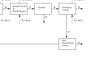
A generalised chemical process control loop [Williams, 1960] is given in Figure 1. The plant considered here is to produce a certain amount of chemical product, P, whose exact nature need not be specified here. We will not consider the detailed chemical kinetics of the reactions involved in producing P. Dynamics of the process is ignored and steady state is assumed for all flows and reactions. This case study is mainly to demonstrate how Z can be applied to the specification of functional behaviour of complex instrument systems, instead of simple instruments such as pressure sensors.

Since flow rates (e.g. in lb/hr) and temperatures (e.g. in o_{C) will be used intensively}

in the following analysis, we first define them as real numbers

FR, T: P R

5.3-1 Reactor

The main chemical reaction of the process occurs in the reactor, which takes initial reactants A and B, and produces a mixture of various chemicals, including A, B and P. We denote the output of chemical mixture as

f

ri. Note that a recycling flow of

f

l also

feeds into the reactor. A flow of water,

f

w1, is used for cooling purpose, with inward

w1o: T

and the operation "React" is specified by

React

f

w2: FR

t

w2i,

t

w2o: T

The operation "Cool Reaction" is described by

CoolReaction

ri?

5.3-3 Decanter

Since G has a considerably higher gravity than the carrier stream, it may be removed by settling in a decanter. No specific state variables are associated with the decanter, and we only specify the decanting operation by the following schema

r?

5.3-4 Distillation Column

(9)

column here. However, since the coolant water temperature is closely related to plant capacity to produce P, we will have to restrict the allowed range of the coolant temperature, say, below 10 o_{C. Let us assume that a stream rate of 5000 lb/hr of P shall}

be produced from the plant. The design of the distillation column will depend on the maximum allowed coolant temperature and the required production rate of P. The state space of the distillation column is given as

DistillationColumn

f

w3: FR

t

w3i,

t

w3o: T

t

w3i ≤ 10

The distillation operation can be specified as

Distill

s, still contains some

(10)

d!

f

p! = 5000

p! = 5000

which can be interpreted into the following statements:

1. The plant is to use chemicals A and B to manufacture chemical product P at a rate of 5000 lb/hr.

(11)

produced and it must be disposed of as a waste material.

3. Apart from product stream P and waste material stream G, there must be a channel for stream D to be discarded.

4. All coolant flowing into the plant must has a constant flow rate and they must be maintained at a constant temperature. In addition, the temperature of the coolant water used in distillation must not exceed 10 o_C.

6. Conclusions

Using formal methods for specification purposes, one can obtain a clear understanding of user's problems, especially the aspects of functional behaviour, and therefore produce a correct specification document based on this understanding. The case studies presented in this paper have demonstrated this point very well. In the meantime, formal verification of specification consistency may be checked using formal proof methods. The task of such verification will not be pursued in this paper.

Formal specifications also provide the basis for formal validation checking and automatic specification-to-product transformation. This advantage is most obvious in software development and digital chip manufacture, though much remains to be explored of formal validation and automatic transformation in measurement instrument development.

7. Acknowledgements

The authors wish to thank the SERC for the SEED research grant. They would also like to express their gratitude to Dr. J. Moffett of Imperial College, for his criticism with respect to Z specifications.

8. References

Balzer R. 1985, A 15 Year Perspective on Automatic Programming, IEEE

Transactions on Software Engineering, Vol.11 No.11

Berg H.K., Boebert W.E., Franta W.R. & Moher T. G . 1982, Formal

Methods of Program Verification and Specification, Prentice-Hall International

Blackburn M.R. 1989, Using Expert Systems to Construct Formal Specifications,

IEEE Expert, Vol. 4 No.1

(12)

Systems, Addison-Wesley

Cook S.C. 1990, A Knowledge-Based System for Computer-Aided Generation of

Measuring Instrument Specifications, PhD thesis, Measurement and Instrumentation

Centre, City University, London

Delisle N. &Garlan D. 1990, A Formal Specification of an Oscilloscope, IEEE

Software, Vol.7 No.5

Finkelstein L. 1987, Instrument and Instrument Systems: Concepts and Principles,

Systems and Control Encyclopedia (editor: M.G. Singh), Pergamon Press

Gehani N.H. & McGettrick A.D. (ed.) 1986, Software Specification Techniques,

Addison-Wesley, pp.173-185

Hall A. 1990, Seven Myths of Formal Methods, IEEE Software, Vol.7 No.5

Hayes I. (ed.) 1987, Specification Case Studies, Prentice-Hall International

Hoare C.A.R. & Gordon M.J.C. (eds.) 1992, The Royal Society Discussion

Meeting on Mechanized Reasoning and Hardware Design, to be published by Prentice-Hall International in June 1992

Morgan C. & Sufrin B. 1984, Specification of the UNIX Filing System, IEEE

Transactions on Software Engineering, Vol.10 No.2

Partsch H. 1983, Program Transformation Systems, ACM Computing Surveys,

Vol.15 No.3

Sommerville I. 1989, Software Engineering, Addison-Wesley

Williams T.J. & Otto R.E. 1960, A Generalized Chemical Processing Model for the

(13)

Figure 1. A Generalised Chemical Process Model for Control

Reactor Reaction Cooler

&

Heat Exchanger

Decanter Distillation

Column

Flow