University of Rhode Island University of Rhode Island
DigitalCommons@URI
DigitalCommons@URI
Open Access Dissertations 2015Goal Representation Adaptive Dynamic Programming for Machine
Goal Representation Adaptive Dynamic Programming for Machine
Intelligence
Intelligence
Zhen NiUniversity of Rhode Island, [email protected]
Follow this and additional works at: https://digitalcommons.uri.edu/oa_diss
Recommended Citation Recommended Citation
Ni, Zhen, "Goal Representation Adaptive Dynamic Programming for Machine Intelligence" (2015). Open Access Dissertations. Paper 351.
https://digitalcommons.uri.edu/oa_diss/351
This Dissertation is brought to you for free and open access by DigitalCommons@URI. It has been accepted for inclusion in Open Access Dissertations by an authorized administrator of DigitalCommons@URI. For more information, please contact [email protected].
GOAL REPRESENTATION ADAPTIVE DYNAMIC PROGRAMMING FOR MACHINE INTELLIGENCE
BY ZHEN NI
A DISSERTATION SUBMITTED IN PARTIAL FULFILLMENT OF THE REQUIREMENTS FOR THE DEGREE OF
DOCTOR OF PHILOSOPHY IN
DEPARTMENT OF ELECTRICAL, COMPUTER AND BIOMEDICAL ENGINEERING
UNIVERSITY OF RHODE ISLAND 2015
DOCTOR OF PHILOSOPHY DISSERTATION OF
ZHEN NI
APPROVED:
Dissertation Committee:
Major Professor Haibo He
Yan Sun Lisa DiPippo Nasser H. Zawia
DEAN OF THE GRADUATE SCHOOL
UNIVERSITY OF RHODE ISLAND 2015
ABSTRACT
This dissertation is focused on a general purpose new framework for machine intelligence based on adaptive dynamic programming (ADP) design. This research is significantly important for developing self-adaptive intelligent system that are highly robust and fault-tolerant to uncertain and unstructured environments. Gen-erally, there are two key components toward building truly self-adaptive systems: fundamental understanding of brain intelligence and complex engineering designs. This dissertation will focus on general purpose computational intelligence method-ologies from a biological inspired perspective, and develop a new self-learning ma-chine intelligent system online over time. Furthermore, this new approach will also be explored on wide critical engineering applications.
Specifically, a new framework, named “goal representation adaptive dynamic programming (GrADP)”, is proposed and introduced in this dissertation. It is regarded as the foundation of building intelligent systems through internal reward learning, goal representation and state-action association. Unlike the traditional ADP design with an action network and a critic network, this new approach inte-grates an additional network, called the reference (or goal) network, such that to build a general internal reinforcement signal. Unlike the traditional fixed or pre-defined reinforcement learning signal, this new design can adaptively update the internal reinforcement representation over time and thus facilitate the system’s learning and optimization to accomplish the ultimate goals.
The original contribution of this research is to integrate an adaptive goal representation design into ADP framework rather than engineering hand-crafted reward functions in literature. This is the first time that the reward signal is presented in a general mapping function by the observation of system variables over time. This is also an important step towards a general purpose self-adaptive
learning system based on ADP designs. Generally, ADP family has three major categories: heuristic dynamic programming (HDP), dual heuristic dynamic pro-gramming (DHP), and globalized dual heuristic dynamic propro-gramming (GDHP). In this research, goal representation principle has been integrated into each de-sign, and verified with promising optimization and learning results. To this end, goal representation heuristic dynamic programming (GrHDP), goal representation dual heuristic dynamic programming (GrDHP), and goal representation global-ized dual heuristic dynamic programming (Gr-GDHP), are successfully proposed and developed as a new GrADP family. Further studies of GrADP approaches from toy problems to real-world applications have been provided in comparison with several other classical control and reinforcement learning approaches. The rigorous mathematical analysis and stability assurance have also been provided to address the convergence and boundedness issues, which are the theoretical assur-ance for this new integrated design. In summary, this is the first time that the new GrADP design framework has been proposed and described explicitly with its family members. The numerical simulation verification, engineering applications and also theoretical results are provided to study each of the new architecture design from different viewpoints.
ACKNOWLEDGMENTS
First and foremost, I would like to express my ernest gratitude to my advisor, Prof. Haibo He, for his continuous and invaluable, guidance, help and support through my Ph.D. study at University of Rhode Island (URI). I still remember his words five years ago: “to be an independent researcher”, which has been the motto in my mind all the way to today. It has been my great honor to be one of his Ph.D. students and work with him on quite many exciting research topics. He not only delivered cutting-edge knowledge in the field to me, but also educated me to be a creative and committed person. His vision towards frontier research directions inspired me to be a self-motivated researcher and keep moving forward in my academic career. His mentorship was paramount in shaping various aspects of my professional career, and his personality was also a remarkable role model in my life. Without those, I would not be so proud of myself as of today.
I also want to sincerely thank for Prof. Yan Sun, Prof. Richard Vaccaro, Prof. Lisa DiPippo, and Prof. P. V. August for serving as my dissertation defense committee. Precious feedback and comments in this process provided me a different view of my research work and myself, which helped this dissertation to be in better shape. Also thanks for Prof. Jinyu Wen and Dr. Danil Prokhorov for close collaborations and suggestions all the way along this research direction.
Special thanks are conveyed to my teammates in Computational Intelligence and Self-Adaptive System (CISA) group in URI throughout my Ph.D. period: Xi-angnan, Yufei, Jing, Jun, Bo, Chris, Chaoxu, Siyao, Lu, Xiao, and many other visiting scholars. Discussions with them provided me lots of inspirations and moti-vations. Also thanks for my close friends Xiaorong, Quan, Fu, Yuhong, Yihai and Daxian, who also made my life in URI colorful and memorable.
for their encouragement. Without them, this work would never come true. Many thanks for their continuous support and love. I would also like to share my every single step forward and achievement all together with them.
TABLE OF CONTENTS
ABSTRACT . . . ii
ACKNOWLEDGMENTS . . . iv
TABLE OF CONTENTS . . . vi
LIST OF TABLES. . . xi
LIST OF FIGURES . . . xiii
CHAPTER 1 Introduction . . . 1
1.1 Motivations and Inspirations . . . 1
1.2 Significance of Self-Adaptive System Designs . . . 2
1.3 Research Objectives . . . 3
1.4 Dissertation Organization . . . 4
2 Background and Literature Discussion . . . 6
2.1 Introduction . . . 6
2.2 Markov Decision Process (MDP) and Reinforcement learning (RL) 6 2.3 Adaptive Dynamic Programming (ADP) Family . . . 8
2.3.1 Model-Based and Model-Free Designs . . . 8
2.3.2 Heuristic Dynamic Programming (HDP) . . . 9
2.3.3 Dual Heuristic Dynamic Programming (DHP) . . . 10
2.3.4 Globalized Dual Heuristic Dynamic Programming (GDHP) 11 2.4 Summary . . . 12
Page
vii
3 A New Internal Goal Representation Framework . . . 13
3.1 Introduction . . . 13
3.2 A Three-Network ADP Architecture . . . 13
3.3 Learning and Optimization Algorithms . . . 15
3.3.1 Learning in Goal Network . . . 17
3.3.2 Learning in Critic Network . . . 19
3.4 Simulation Studies . . . 20
3.4.1 Cart-Pole Balancing Example . . . 21
3.4.2 Triple-Link Inverted Pendulum Balancing Example . . . 23
3.5 Summary . . . 33
4 Goal Representation Design for Heuristic Dynamic Program-ming (GrHDP) Architecture . . . 34
4.1 Introduction . . . 34
4.2 Design of GrHDP for Tracking Control . . . 34
4.2.1 Design of Dual-Critic Network . . . 35
4.2.2 Design of Tracking Filter . . . 37
4.2.3 Design of Reinforcement Signals . . . 39
4.3 Association and Implementation . . . 39
4.3.1 Learning and Optimization in Dual Critic Network . . . 40
4.3.2 Interaction in Action Network and Tracking Filter . . . . 46
4.4 Simulation Studies . . . 48
4.4.1 Tracking Control Problem with Disturbance . . . 49
4.4.2 Adaptive Signal Tracking Control Problem . . . 52
Page
4.4.4 Virtual Reality Demonstration with Unknown Disturbances 58
4.5 Summary . . . 59
5 Goal Representation Design for Dual Heuristic Dynamic Programming (GrDHP) Architecture . . . 61
5.1 Introduction . . . 61
5.2 Design of the GrDHP Framework . . . 61
5.3 Learning Process of the GrDHP Design . . . 65
5.3.1 Design of Goal Representation in HDP . . . 66
5.3.2 Design of General Utility Representation in DHP . . . . 67
5.3.3 Online Learning in Critic Network . . . 68
5.3.4 Online Learning in Action Network . . . 70
5.4 Simulation Studies . . . 70
5.4.1 Ball and Beam Balancing Example . . . 71
5.4.2 Triple-link Inverted Pendulum Balancing Example . . . . 74
5.5 Discussion of Advanced GrADP Designs . . . 75
5.6 Summary . . . 81
6 Hierarchical Goal Representation Heuristic Dynamic Pro-gramming Design. . . 82
6.1 Introduction . . . 82
6.2 Design of Hierarchical HDP Structure . . . 82
6.2.1 Learning and Adaptation in Hierarchical Goal Networks . 84 6.2.2 Learning and Adaptation in the Critic Network . . . 86
6.2.3 Learning and Adaptation in the Action Network . . . 87
Page
ix
6.3.1 Experiment Configuration and Parameters . . . 87
6.3.2 Simulation Results and Analysis . . . 89
6.4 Summary . . . 93
7 Applications: From Toy Problems to Real-World Applications 97 7.1 Introduction . . . 97
7.2 Maze Navigation Application . . . 97
7.2.1 Maze Navigation Learning Algorithm Description . . . . 97
7.2.2 Maze Navigation Environment Setup . . . 99
7.2.3 Simulation Studies and Analysis . . . 101
7.3 Smart Grid Application . . . 105
7.3.1 Multimachine Power System Environment Setup . . . 109
7.3.2 Simulation Studies and Analysis . . . 110
7.4 Summary . . . 115
8 Conclusions and Future Research Directions . . . 121
8.1 Conclusions . . . 121
8.2 Original Contributions . . . 121
8.3 Future Research Directions . . . 123
LIST OF REFERENCES . . . 125
APPENDIX A Pseudo Code of GrHDP based Tracking Control Algorithm . 139 B Stability Analysis for GrHDP-based Tracking Control . . . . 143
Page
C.1 Problem Formulation . . . 152
C.2 Analysis of GrADP based Learning Approach . . . 155
D Abbreviations . . . 161
LIST OF TABLES
Table Page
3.1 Summary of the parameters used in cart-pole balancing task . . 21
3.2 Performance evaluation on case I: cart-pole balancing task. The
2nd and the 3rd columns are with our proposed method, while the 4th and the 5th columns are the results from existing approach 22
3.3 System constants for the triple link inverted pendulum problem 25
3.4 Summary of the parameters used in triple-link inverted
pendu-lum balancing task . . . 28
3.5 Performance evaluation on case II: triple-link balancing task.
The 2nd and the 3rd columns are with our proposed method, while the 4th and the 5th columns are the results from existing
approach . . . 29
4.1 Summary of the parameters used in the simulation study one . 49
4.2 Summary of the parameters used in the simulation study two . 56
4.3 Summary of total tracking error for the simulation cases . . . . 57
5.1 Comparison of the statistical simulation results on the
triple-link inverted pendulum balancing task with the DHP and the
GrDHP approaches. . . 77
6.1 Summary of the parameters used in the simulation . . . 88
6.2 Simulation results on ball-and-beam balancing task. The 1st
column is with the noise type. The 2nd column is with
Algorithm0, while the 3rd column is with Algorithm1 and the
4th column is withAlgorithm2. The number of trials and
stan-dard deviation are calculated based on the successful runs . . . 91
7.1 Summary of the parameters used in the GrHDP/HDP
con-troller. The notations are kept the same as those in Chapter 3 . . . 110
Table Page
7.2 Summary of the parameters used in the GrHDP/HDP
con-troller. The notations are kept the same as those in Chapter 3 . . . 113
7.3 The admittance matrices between each line/bus in the
three-machine nine-bus system. . . 118
7.4 The per unit value for the parameters of each generator/bus in
the system. . . 119
LIST OF FIGURES
Figure Page
2.1 The schematic diagram of typical model-free HDP structure. . . 10
2.2 The schematic diagram of typical DHP structure. . . 11
2.3 The schematic diagram of typical GDHP structure. . . 12
3.1 The proposed ADP architecture with internal goal representation. 14
3.2 Parameters adaptation and tuning based on backpropagation . 16
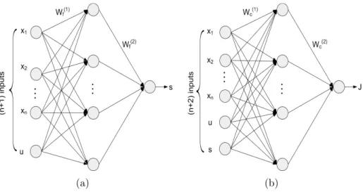
3.3 Design of the three networks with nonlinear neural network: (a)
Reference network design; (b) Critic network design . . . 17
3.4 Definition of notation used in the system equations for the triple
link inverted pendulum benchmark . . . 23
3.5 Statistics of the successful runs. (a) Number of required trials
for the successful runs. (b) Histogram the statistics. . . 29
3.6 Typical trajectory on the triple-link inverted pendulum
balanc-ing task. (a) The position x of the cart. (b) The 1st joint angle of the triple link pendulum. (c) The 2st joint angle of the triple link pendulum. (d) The 3st joint angle of the triple link pen-dulum. (e) The velocity of the cart. (b) The angular velocity of the 1st joint angle of the triple link pendulum. (c) The an-gular velocity of the 2st joint angle of the triple link pendulum. (d) The angular velocity of the 3st joint angle of the triple link
pendulum. . . 30
3.7 Typical histogram on the triple-link inverted pendulum
balanc-ing task. (a) The histogram of position x of the cart. (b) The histogram of the 1st joint angle of the triple link pendulum. (c) The histogram of the 2st joint angle of the triple link pendu-lum. (d) The histogram of the 3st joint angle of the triple link
pendulum. . . 31
3.8 Typical trajectory of cost-to-go and control action signal on the
triple-link inverted pendulum balancing task. (a) The cost-to-go
signal on the task. (b) The control action signal on the task. . . 32
Figure Page
4.1 Architecture design of the proposed HDP approach with a
track-ing filter. . . 35
4.2 Description of the dual critic network. . . 36
4.3 Description of the tracking filter. . . 37
4.4 Learning schematic in dual critic network. . . 40
4.5 (a) The neural network structure of the reference network; (b) The neural network structure of the critic network. . . 42
4.6 (a) The neural network structure of the action network; (b) The control action generator. . . 48
4.7 The typical tracking performance with our proposed approach. . 50
4.8 The typical tracking performance with HDP approach . . . 51
4.9 The typical tracking performance with our proposed approach. . 53
4.10 The typical tracking performance with HDP approach. . . 54
4.11 A schematic diagram of ball-and-beam system . . . 55
4.12 The typical tracking performance with our proposed approach. . 56
4.13 The typical tracking performance with HDP approach . . . 57
4.14 The schematics of virtual reality demonstration platform. . . 59
4.15 The typical tracking performance with the proposed approach in VR/Simulation platform . . . 59
5.1 The conceptual diagram of the GrDHP architecture. Solid ar-rows refer to the signal paths, while the dash arar-rows refer to the backpropagation paths. . . 62
5.2 The learning flowchart in the GrDHP design. The neural net-works are represented with their corresponding weights and these weights are carried on throughout the learning process. The subscript number under each parameter (e.g., r) refers to time step. . . 63
Figure Page
xv
5.3 The proposed architecture of the GrDHP design. Solid/Bolded
arrows refer to the signals/vectors and dash arrows refer to the weights tuning paths. ∂x∂r((tt)) and ∂r∂u((tt)) refer to the partial
deriva-tives of the external reward/utility w.r.t the system state x(t)
and the control action u(t), respectively.The block DER
imple-ments (5.9). . . 65
5.4 Comparison of the statistical results on the ball-and-beam
bal-ancing task with both the GrDHP and the DHP approaches. . . 72
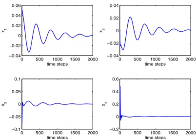
5.5 Typical trajectories of the state vectors in the first 2000 time
steps in a typical successful trial. . . 73
5.6 The weights evolution of the goal network in the first 1000 steps
in a typical successful trial. . . 74
5.7 Typical trajectories of the angles in a successful trial under the
condition of noise free. . . 75
5.8 Typical trajectories of the λ (corresponding to the angles in
Fig.5.7) in a successful trial under the condition of noise free. . 76
5.9 The typical trajectory of the control force (Newton) applied on
the cart in a successful trial under the condition of noise free. . 78
5.10 The histogram of the control force (Newton) applied on the cart
(corresponding to the trajectory in Fig.5.9). . . 79
6.1 The schematic of hierarchical HDP structure . . . 83
6.2 Cascading weights tuning path inside the goal generator . . . . 84
6.3 The typical trajectory of x1 and x2 with Algorithm 2 . . . 89
6.4 The histogram of x1 in a typical successful run with Algorithm 2 90
6.5 The typical trajectory of x3 and x4 with Algorithm 2 . . . 91
6.6 The typical trajectory of the control action and the total
cost-to-go signal with Algorithm 2 . . . 92
6.7 The typical trajectory of internal goal signals with Algorithm 2 93
Figure Page
6.9 The boxplot of the required number of trials in 100 random runs
with Algorithm 0, Algorithm 1 and Algorithm 2. . . 95
6.10 The typical trajectory of control action with Algorithm 2 under
5% uniform noise on the actuator . . . 95
6.11 The typical trajectory of the state vectors x1 and x2 with
Algo-rithm 2 under 5% uniform noise on the sensor of the position of
the ball . . . 96
7.1 Simulation setup: flowchart of the GrHDP approach on maze
navigation problem. Value table is updated at the end of each trial. The learning process will be terminated when the trial number reaches the maximum trial number. . . 100
7.2 Learning curves with GrHDP, HDP, Sarsa(λ) and Q-learning
approaches in 16 * 16 maze navigation. GrHDP approach shows the fastest learning speed and lowest final sum of square error
than the other three approaches. . . 103
7.3 Surface plot of the value table learned by GrHDP approach on
maze navigation problem (16*16). x and y axis refer to the
coordinates of the agent while z axis refers to the J-value. . . . 104
7.4 Diagram of 3-D maze (5*5*5) navigation benchmark. The goal
locates at the upper-right corner of the maze and the agent needs to try 6 directions before it can learn the policy. . . 105
7.5 Learning curves with GrHDP, HDP, Sarsa(λ) and Q-learning
approaches in 5*5*5 maze navigation. GrHDP approach shows the fastest learning speed and lowest final sum of square error
than the other three approaches. . . 106
7.6 The schematic diagram of the three-machine nine-bus power
sys-tem. The dot lines show the observations from each generator. The ADP controller provides three supplementary control sig-nals for three generators respectively based on these (delayed)
Figure Page
xvii
7.7 The schematic diagram for a single generator. The ADP and
PSS controller will be connected into the closed-loop if S1 switches to 1 or 2. The dot arrows show the observed signals from the generator and the grid, while the solid arrows show the signal paths. . . 109
7.8 The data flowchart of GrHDP controller with neural network
implementation. . . 111
7.9 Damping performance on ∆ω12under three-phase-ground fault.
Four approaches are compared on the same environment settings.114
7.10 Damping performance on ∆ω13under three-phase-ground fault.
Four approaches are compared on the same environment settings.115
7.11 Damping performance on ∆ω23under three-phase-ground fault.
Four approaches are compared on the same environment settings.116
7.12 Comparison of the control performance on the output active
power P e1 under both −5% and +5% step changes . . . 117
7.13 Comparison of the control performance on the output active
power P e2 under both −5% and +5% step changes. . . 117
7.14 Comparison of the control performance on the output active
power P e3 under both −5% and +5% step changes. . . 118
7.15 The output active power P e1 under the load fluctuations. The
GrHDP approach is compared against the other three
ap-proaches under the same sequential load disturbances. . . 119
7.16 The supplementary control signals u1, u2 and u3 provided by
CHAPTER 1 Introduction
1.1 Motivations and Inspirations
Brain intelligence and animal intelligence are very important biological in-spiration to develop truly self-adaptive systems to such a level of intelligence in certain perspectives [1, 2, 3]. Although many important fundamental researches and critical engineering applications have been successfully developed, there is still a long way to achieve the general-purpose intelligent machine in an engineer-ing way. One of the key challenges is how to design the intelligent systems to have the capacity to learn, predict and optimize over time, in order to achieve the ultimate goals [4, 5, 6, 7, 8]. In this dissertation, a new data-driven framework based on adaptive dynamic programming (ADP) will be proposed to help the in-telligent system to learning to optimize online in the uncertain and unstructured environment. A further hierarchical data-driven framework will also be provided to mimic brain intelligence to help achieve the long-term goal through multi-stage internal short-term goals from a biological viewpoint.
In the traditional ADP and reinforcement learning (RL) design, the reinforce-ment signal feedback is usually set as a fixed formula, such as a binary value or the quadratic functions. These are defined according to designers’ past experience and the prior knowledge of the systems under control. For instance, in two important editorial research books [9, 10], many researchers and professors are designing the reward feedback based on their knowledge of the system, including several complex engineering problems. Other research works [11, 12, 13, 14] connected this reward design with the control problem and thus define it as a quadratic function (or the integration in a continuous time format). Although promising results have been reported, there is still an opportunity to address this issue from a more general
way [15, 16, 17].
To this end, I am motivated to introduce a general-purpose reinforcement sig-nal representation that is applicable for general systems without any prior knowl-edge and past experience. This general reinforcement signal feedback design will be able to help providing an adaptive internal goal guidance online over time, in order to best fit the online operation environment. For example, if the objectives change over time, the reinforcement signal feedback should also be adjusted to fit the new objective [18, 19, 20]. Or, if there are some disturbances or noises during the operation, the reinforcement signal feedback should also be adjusted to provide the best representation. More importantly, I am inspired by biological systems that have multi-level and multi-stage internal goals to accomplish, in or-der to achieve the long-term goal [21, 22, 23]. For instance, if an animal wants to survive in a hostile environment, it needs to consider the trade-off between getting the food and escaping from a hunter. Motivated by such observations, a multi-level reinforcement signal representation is proposed to build a value system that can facilitate the development of hierarchical internal goal representation. The learning and association in both top-down and bottom-up pathways to support this intelligent decision-making process is also discussed here. Based on all these literature search and biological inspiration, a new adaptive learning framework for machine intelligence based on adaptive dynamic programming is introduced in this dissertation.
1.2 Significance of Self-Adaptive System Designs
This is the first time that a self-adaptive reinforcement signal design has been proposed and demonstrated in the community of ADP and RL. The significance of the results provided in this dissertation is summarized as following:
• This research proposes a new self-adaptive learning architecture for machine
intelligence based on adaptive dynamic programming technique. The online learning for the internal reinforcement signal is conducted with environment uncertainties over time. This architecture is a very important step ahead for the general-purpose machine intelligent system designs.
• Multi-stage hierarchical reinforcement signal representation has been
pro-posed to handle the multi-stage short-term goals in the biological systems, in order to accomplish long-term objectives. This is the first time that multi-stage reinforcement signals design have been proposed based on adaptive dynamic programming architecture.
• The reinforcement signal representation, also called goal representation, is
fully applied to the existing designs in adaptive dynamic programming family. It is thus called goal representation adaptive dynamic programming (GrADP) design family. Such designs have been applied in several critical engineering applications to mimic certain level of human brain and animal behaviors.
1.3 Research Objectives
The objective of this dissertation is focused on designing general-purpose in-telligent systems that are capable to learn to optimize the decision-making process in an unknown environment, based on the biological inspired multi-stage internal goal representations. It is very important to justify the objectives of this inte-grated framework via different types of ADP architectures onto the various critical engineering applications:
• The goal representation design could be able to learn proper internal reward
through the interaction with the environment adaptively, rather than a fixed reward formula all the way over time.
unknown environment under disturbances, noises and uncertainties. The control policy could be better fitted through the online adjustment.
• The designed hierarchical goal representation could be able to provide
multi-stage internal reward signals for the intelligent systems, to mimic certain-level of intelligence in biological systems.
• The proposed new framework could be able to be implemented in scalable
hardware embedded systems, including FGPA board and GPU board, bring such intelligence into real-world applications.
1.4 Dissertation Organization
This dissertation will be organized as following:
Chapter 2 provides the background of my research and literature review in current community. It further provides the introduction Markov decision process, reinforcement learning, and the ADP design family.
Chapter 3 focuses on a new internal goal representation design based on the
traditional ADP architecture. An additional reference/goal network has been
added into this structure, and the performance is verified through two balancing benchmarks.
Chapter 4 discusses a new tracking control scheme based on the dual-critic ADP architecture (i.e., critic and reference networks). The design and implemen-tation of dual-critic network, action network and tracking filter are presented. The comparative performance is also provided via several tracking examples.
Chapter 5 presents the integration of a general utility function representation onto the DHP design. The explicit internal utility function is provided by the goal network and thus its derivatives can be adaptively adjusted. The learning capacity of the proposed DHP design is improved and demonstrated via the commonly used
balancing benchmarks.
Chapter 6 further provides the integration of multi-level goal representation design onto HDP architecture, which is also called hierarchical HDP design. This hierarchical design is demonstrated with the significant control improvement in comparison with classical HDP and goal representation HDP designs from certain perspectives.
Chapter 7 provides the applications of the proposed goal representation adap-tive dynamic programming design family from toy problems (maze navigation), to real-world applications (multi-machine power system stability and control).
Chapter 8 concludes the dissertation and also discusses the future directions of this self-adaptive learning framework based on adaptive dynamic programming.
CHAPTER 2
Background and Literature Discussion
2.1 Introduction
Markov decision process (MDP) is a long-standing research topic in decision making models in stochastic process [24, 25, 26]. Value function (or state-action pair) is usually used to evaluate how good it is of the agent for a given state. If the state and the action spaces are finite, then it is called finite MDP, which is particularly important to the theory of reinforcement learning [27, 28, 16].
In this chapter, the background of both MDP and reinforcement learning will be introduced. The design architectures and differences of both model-based and model-free ADP will be discussed. I will also discuss the current literature review of the ADP designs among three major categories, i.e., heuristic dynamic programming, dual heuristic dynamic programming and globalized dual heuristic dynamic programming, as the background of this research.
2.2 Markov Decision Process (MDP) and Reinforcement learning (RL)
A Markov decision process is denoted as a tuple X, U, r, P, where X is the
state space, U is the action space, P is the transition probability and r is the
reward feedback [29, 2, 30]. For instance, given any state and action,x andu, the
probability of each possible next state x0 is defined as
Pxxu0 = Pr{xt+1=x0|xt =x, ut=u}. (2.1)
While the expected value of the next reward is defined as
Ruxx0 =E{rt+1|xt =x, ut=u, xt+1=x0}. (2.2)
Solving a reinforcement learning task means finding a policy that achieves the maximum reward feedback in the long-run. There is always at least one policy
that is better or equal than any other policies, and this is call optimal optimal
policy [31, 32, 33]. In literature, π is defined as policy and π∗ is denoted as the
optimal policy (although there may be more than one). The value of a state x
under a policy π is defined as
Vπ(x) = Eπ{Rt|xt=x}=Eπ nX∞ k=0 {{γkrk+1|xt =x}} o . (2.3)
whereEπ is the expected value given that the agent follows policyπ. The objective
in this process is to find the optimal policyπ∗so that to achieve the optimalVπ∗(x) as V∗(x) = max π V π (x) = max u X x0 n Pxxu0 Ruxx0 +γVπ ∗ (x0) o . (2.4)
In optimal control area [34, 35, 2], Bellman’s optimality principle suggests that an optimal policy can be built for the “tail subproblem” involving the last stage and extended backward until that the optimal strategy is built for the entire process. With the notations in (2.1) and (2.2), Bellman’s optimality equation for
Q∗ can be written as Q∗(x, u) = X x0 Pxxu0 h Ruxx0 +γmax u0 Q ∗ (x0, u0)i. (2.5)
where Q∗(x, u) refers to the value function of the current state x and Q∗(x0, u0)
refers to the value function of the possible next statex0. Equations (2.4) and (2.5)
are actually two forms of Bellman optimality presentations.
In past decades, RL, especially Q-learning and temporal difference (TD) learn-ing, has been employed to solve Bellman’s equation in MDP. For instance, in [36], a robust reinforcement learning approach, basically Q-learning approach, was pro-posed to help the agent to find the optimal control policy with minimum cost. In addition, “Dyna-Q” learning architecture was later introduced in [37]. This architecture can be integrated with trial-and-error (reinforcement) learning and execution-time planning, into a single process operation alternately on the world
and on a learned model of the world. Furthermore, TD(λ) was also developed to improve the convergence speed on solving MDP problems in [38, 39, 24, 40, 41]. Meanwhile, ADP has demonstrated the capability to find the optimal control pol-icy over time and solve the Bellman’s equation in a principle way. High-level understanding of ADP [42, 43, 44, 45, 46, 47], implied that ADP approaches could be able to learn and optimize the control policy over time, and find the solution for Bellman’s optimality equation efficiently. Various ADP architectures, includ-ing heuristic dynamic programminclud-ing (HDP), dual heuristic dynamic programminclud-ing (DHP), and globalized dual heuristic dynamic programming (GDHP) (together with their action-dependent (AD) versions), have been proposed in [48, 29] to seek the optimal policy over time. It has also been demonstrated that HDP has the similar learning and association principle with the Q-learning algorithm.
2.3 Adaptive Dynamic Programming (ADP) Family
2.3.1 Model-Based and Model-Free Designs
In this ADP design family, there are usually two major architectures: model-based ADP architecture and model-free ADP architecture. In the model-model-based architecture, a model-network is used to predict the future system variables and the corresponding future value function (or future derivatives of value function). Moreover, this model network is also used to connect action and critic networks during the back-propagation process. In the model-free architecture, the temporal difference error will be achieved by the current time step and the previous time step. In this case, there is no need to use the model network to predict for the future system variables (or the future vale function). The back-propagation process is thus simplified without any usage of model network. Such model-free HDP has also been regarded as the equivalence to the classical Q-learning approach. More importantly, both versions have been used for various real-world applications with
successful results, and also been applied on the ADP design family. For instance, the online model-free HDP was developed in [49, 50, 51], where the authors took the advantages of the potential scalability of the adaptive critic designs and the intuitiveness of Q-learning. It is also an online learning scheme that simultaneously updates the value function and the control policy. The model-based HDP was also proposed with rigorous convergence proof to solve the optimal control problem for discrete-time nonlinear systems [52]. For model-based DHP/GDHP design, the authors in [12, 53] introduced that the efficient learning can be achieved with different weights for different error terms on the auto-lander helicopter problem. In [54, 55, 56], the authors also demonstrated the convergence analysis for model-based DHP/GDHP in terms of cost function and control law.
2.3.2 Heuristic Dynamic Programming (HDP)
Heuristic dynamic programming is the most basic architecture in the ADP family [57, 58]. There are usually two networks in model-free heuristic dynamic programming design, as presented in Fig. 2.1. An action network is used to provide the control action to the system, and a critic network is used to evaluate the control performance over time. For example, the action network will generate the control
action u based on the observation of the system variables x. The critic network
will evaluate the performance of this control policy based on the reinforcement
signal feedback r from the environment. Meanwhile, the value function J will
be approximated by the critic network. As presented in Fig. 2.1, the objective function of critic network will be provided by the temporal difference between current step and previous step in Bellman’s equation, denoted as
The objective function for the action network is to minimize the total cost (or maximize the total reward), denoted as
ea(t) = J(t)−Uc (2.7)
where Uc is the ultimate (expected) cost function and J function is expected to
approach this expected value.
Figure 2.1. The schematic diagram of typical model-free HDP structure.
2.3.3 Dual Heuristic Dynamic Programming (DHP)
Dual heuristic dynamic programming belongs to the advanced ADP design [59, 60]. As presented in Fig. 2.2, there are still one action network and one critic network in the design, and the action network is used to generate control actions. Yet, the critic network is used to approximate the derivatives of the value
function λ rather than value function itself. The evaluation criteria is said to be
more accurate in this case. Usually, there is a model network in DHP design. This model network is required to be trained offline based on the input and output data from the system, and then applied online to predict the future system variables
(e.g., ˆx(t + 1) and ˆu(t + 1)). In the backward process, the model network is
also used as a bridge to connect the weights propagation from critic network to action network. Note that, the partial derivatives of value function is defined as
λ= [∂J∂x((tt)) ∂J∂u((tt))]. Thus the error function of critic network is defined as
ec(t) = ∂J(t) ∂Y(t) −α ∂J(t+ 1) ∂Y(t) − ∂r(t) ∂Y(t) (2.8) 10
where Y(t) = [x(t) u(t)]T. The error function of action network can be directly
obtained fromλ as
ea(t) =α
∂Jˆ(t+ 1)
∂u(t) (2.9)
In recent literature, model-free DHP has also been proposed with finite differ-ence technique on various balancing examples [61]. This approach has also been demonstrated with efficient computational time cost.
Figure 2.2. The schematic diagram of typical DHP structure.
2.3.4 Globalized Dual Heuristic Dynamic Programming (GDHP)
Globalized dual heuristic dynamic programming is the most advanced ADP design [59, 60]. As seen from Fig. 2.3, it has very similar structure with DHP, i.e., it has an action network to generate control action, yet a critic network to approximate both the value function and its derivatives (one may see that there are two dash lines to). Model network is also usually applied in GDHP design, as it is used to predict the future system variables and the corresponding future value function (with its derivatives). Though GDHP is regarded to be the most accurate ADP learning control approach, it generally has more computational cost and complicated learning algorithms than those with HDP and DHP. The error function of critic (action) network is the error combination of the previously introduced HDP and DHP designs, and thus the learning algorithm is more complicated. It is always a tradoff to choose between advanced ADP designs (i.e., DHP and GDHP)
and basic ADP design (i.e., HDP) for a specific system.
Figure 2.3. The schematic diagram of typical GDHP structure.
2.4 Summary
This chapter presents the background knowledge and literature discussion for adaptive dynamic programming and reinforcement learning, which are both deeply indebted to the idea of Markov decision processes from the field of optimal control. The background of learning and association (i.e., state-action pair) in decision-making process is provided. The fundamental principles of reinforcement learning and adaptive dynamic programming are also discussed. Three major architectures in adaptive dynamic programming are introduced to solve the Bellman’s equation and find the optimal control policies.
In the rest of this dissertation, new ADP architectures are proposed based on the presented knowledge and principle in this chapter, and improved learning control results from toy problems to real-world applications will also be provided.
CHAPTER 3
A New Internal Goal Representation Framework
3.1 Introduction
In this chapter, a novel adaptive dynamic programming architecture with three neural networks, i.e., an action network, a critic network, and a reference network, is developed with internal goal-representation technique for online learn-ing and optimization [62, 63]. Unlike the traditional ADP design with two neural networks (i.e., an action network and a critic network), this approach integrates the third neural network, called the reference network, into the actor-critic design framework. The motivation is to build a general-purpose (internal) reinforcement signal to facilitate learning and optimization overtime [6, 7, 5]. The detailed de-sign procedure and its associated learning algorithm are provided to explain how the effective learning and optimization can be achieved. Furthermore, the learn-ing control performance on two commonly used balanclearn-ing benchmarks are also presented.
3.2 A Three-Network ADP Architecture
Fig. 3.1 shows the proposed ADP architecture with goal representation net-work [62, 63]. Compared to the existing ADP architectures [64, 65, 66, 67], the key
idea is to integrate another neural network, the reference network, to provide the
internal reinforcement signal (internal goal representation) s(t). By introducing
such a reference network to represent the system’s internal goal, this architecture provides a new way to adaptively estimate the internal reinforcement signal in-stead of crafted by hands. This is the most important contribution of this work when compared to the existing ADP designs. From a mathematical point of view, this new architecture presents two major differences compared with that of the
existing ADP designs. First, the critic network has one more additional inputs(t) from the reference network. Second, the optimization error function and learning in the reference network and critic network are different: The error function of
the reference network is related to the primary reinforcement signalr(t), whereas
for the critic network, it is related to the internal reinforcement signal s(t). Both
of these characteristics will change the parameters tuning and adaptation. Note that another characteristic of this method is that it shares the advantage of no requirement of a system model to predict the future system state, as proposed in the important ADP architecture in [68, 69]. This means similar to the architecture in [68], the proposed approach also stores the previous cost-to-go value to obtain the temporal difference for training at any time instance. This enables the online learning, association, and optimization over time.
Figure 3.1. The proposed ADP architecture with internal goal representation.
3.3 Learning and Optimization Algorithms
From Fig. 3.1 one can see, there are three paths to tune the parameters of the three types of networks. The action network in this architecture is similar to the classic ADP approach to indirectly backpropagate the error between the
desired ultimate objective Uc and the J function from the critic network [68][70].
Therefore, the error function Ea(t) used to update the parameters in the action
network can be defined as (path 1 in Fig. 3.1):
ea(t) = J(t)−Uc(t); Ea(t) =
1 2e
2
a(t). (3.1)
The key of this architecture relies on the learning and adapting process for the
reference network and critic network. As the primary reinforcement signal r(t) is
presented to the reference network, the secondary (also called internal)
reinforce-ment signal s(t) is adapted to provide a more informative internal reinforcement
representation to the critic network, which in turn is used to provide a better
ap-proximation of the J(t). In this way, the primary reinforcement signal r(t) is in a
higher hierarchical level and can be a simple binary signal to represent “good” or
“bad”, or “success” or “failure”, while the secondary reinforcement signals(t) can
be a more informative continuous values for improved learning and generalization
performance. Therefore, the error function Ef(t) used to update the parameters
in the reference network can be defined as (path 2 in Fig. 3.1):
ef(t) =αJ(t)−[J(t−1)−r(t)]; Ef(t) =
1 2e
2
f(t). (3.2)
Once the reference network outputs thes(t) signal, it will be used as an input
to the critic network, and also used to define the error function to adjust the parameters of the critic network (path 3 in Fig. 3.2).
ec(t) = αJ(t)−[J(t−1)−s(t)]; Ec(t) =
1 2e
2
c(t). (3.3)
In this architecture, the chain backpropagation rule is used for training and adaptation of the parameters of all three networks. Fig. 3.2 shows the three backpropagation paths used to adapt the parameters in the three networks.
Figure 3.2. Parameters adaptation and tuning based on backpropagation
In this figure, the optimization error functions for the action network Ea,
reference network Ef, and critic network Ec are defined in equations (3.1), (3.2)
and (3.3), respectively. Therefore, chain backpropagation can be calculated
through the three data paths as highlighted in Fig. 3.2. Briefly speaking, the high level conceptual calculation on this can be summarized as follows.
Path 1 For action network:
∂Ea(t) ∂wa(t) = ∂Ea(t) ∂J(t) ∂J(t) ∂u(t) ∂u(t) ∂wa(t) (3.4)
Path 2 For reference network:
(a) (b)
Figure 3.3. Design of the three networks with nonlinear neural network: (a) Ref-erence network design; (b) Critic network design
∂Ef(t) ∂wf(t) = ∂Ef(t) ∂J(t) ∂J(t) ∂s(t) ∂s(t) ∂wf(t) (3.5)
Path 3 For critic network:
∂Ec(t) ∂wc(t) = ∂Ec(t) ∂J(t) ∂J(t) ∂wc(t) (3.6)
3.3.1 Learning in Goal Network
Fig. 3.3(a) shows the reference network used in this design with a 3-layer nonlinear architecture (with 1 hidden layer). To calculate the backpropagation,
we first need to define the reference network outputs(t) as follows.
s(t) = 1−exp −k(t) 1 +exp−k(t). (3.7) k(t) = Nh X i=1 wf(2) i (t)yi(t), (3.8)
yi(t) = 1−exp−zi(t) 1 +exp−zi(t), i= 1, . . . , Nh (3.9) zi(t) = n+1 X j=1 wf(1) i, j(t)xj(t), i= 1, . . . , Nh (3.10)
Where zi is the ith hidden node input of the reference network and yi is the
corresponding output of the hidden node,k is the input to the output node of the
reference network before the sigmoid function,Nh is the number of hidden neurons
of the reference network, and (n+ 1) is the total number of inputs to the reference
network including the action value u(t) from the action network.
To apply the backpropagation rule, one can refer to Fig. 3.2 and equations (3.2) and (3.5). Specifically, since the outputs(t) is an input to the critic network, backpropagation can be applied here through the chain rule (path 2) to adapt the
parameters Wf. This procedure is illustrated as follows.
(1) ∆w(2)f : Reference network weight adjustment for the hidden to the output
layer. ∆w(2)f i =ηf(t)[− ∂Ef(t) ∂wf(2) i (t) ] (3.11) ∂Ef(t) ∂wf(2) i (t) = ∂Ef(t) ∂J(t) ∂J(t) ∂s(t) ∂s(t) ∂k(t) ∂k(t) ∂wf(2) i (t) (3.12) = αef(t)· Nh X i=1 [w(2)c i (t) 1 2(1−p 2 i(t))w (1) ci, n+2(t)]· 1 2(1−(s(t)) 2)·y i(t)
(2) ∆w(1)f : Reference network weight adjustments for the input to the hidden layer.
∆wf(1) i, j =ηf(t)[− ∂Ef(t) ∂wf(1) i, j(t) ] (3.13) 18
∂Ef(t) ∂w(1)f i, j(t) = ∂Ef(t) ∂J(t) ∂J(t) ∂s(t) ∂s(t) ∂k(t) ∂k(t) ∂yi(t) ∂yi(t) ∂zi(t) ∂zi(t) ∂wf(1) i, j(t) (3.14) = αef(t)· Nh X i=1 [w(2)ci (t)1 2(1−p 2 i(t))wc(1)i, n+2(t)]· 1 2(1−(s(t)) 2)·w(2) fi (t) ·1 2(1−y 2 i(t))·xj(t)
Once the reference network provides the secondary reinforcement signal s(t)
to the critic network, one can adapt the parameters in the critic network.
3.3.2 Learning in Critic Network
Fig. 3.3(b) shows the critic network used in our current design with a 3-layer nonlinear architecture (with 1 hidden layer). To calculate the backpropagation,
we first need to define the critic network outputJ(t) as follows.
J(t) = Nh X i=1 wc(2) i (t)pi(t), (3.15) pi(t) = 1−exp−qi(t) 1 +exp−qi(t), i= 1, . . . , Nh (3.16) qi(t) = n+2 X j=1 w(1)ci, j(t)xj(t), i= 1, . . . , Nh (3.17)
Where qi and pi are the input and output of the ith hidden node of the critic
network, respectively, and (n+ 2) is the total number of inputs to the critic
net-work including the action value u(t) from the action network and the secondary
reinforcement signal s(t) from the reference network.
By applying chain backpropagation rule (path 3), the procedure of adapting parameters in the critic network is summarized as follows.
(1) ∆wc(2): Critic network weight adjustments for the hidden to the output layer. ∆w(2)c i =ηc(t)[− ∂Ec(t) ∂wc(2)i (t) ] (3.18) ∂Ec(t) ∂wc(2)i (t) = ∂Ec(t) ∂J(t) ∂J(t) ∂w(2)ci (t) =αec(t)·pi(t) (3.19)
(2) ∆wc(1): Critic network weight adjustments for the input to the hidden layer.
∆w(1)ci, j =ηc(t)[− ∂Ec(t) ∂wc(1)i, j(t) ] (3.20) ∂Ec(t) ∂wc(1)i, j(t) = ∂Ec(t) ∂J(t) ∂J(t) ∂pi(t) ∂pi(t) ∂qi(t) ∂qi(t) ∂w(1)ci, j(t) =αec(t)·w(2)ci (t)· 1 2(1−p 2 i(t))·xj(t) (3.21) 3.4 Simulation Studies
The proposed three-network algorithm has been implemented on a cart-pole balancing problem, which is the same as that in [68]. The ultimate goal here is to control the force applied on the cart to move it either left or right to keep the balance of the single pole mounted on the cart. The system function of the model is described as following: ∂2θ/∂t2 = gsinθ+ cosθ[−F−mlθ˙2sinθ+µ csgn( ˙x)] mc+m − µpθ˙ ml l(43 −mcosθ2 mc+m) (3.22) ∂2x/∂t2 = F +ml[ ˙θ 2sinθ−θ¨cosθ]−µ csgn( ˙x) mc+m (3.23)
where the acceleration g = 9.8m/s2, the mass of the cart m
c = 1.0kg, the mass
of the pole m = 0.1kg, half-pole length l = 0.5m, the coefficient of friction of the
cart µ= 0.0005 and the coefficient of friction the pole µp = 0.000002. The force
F applied to the cart is either 10 Newtons or −10 Newtons, and the sgnfunction in equation (3.23) is defined as following:
sgn(x) = 1, x >0 0, x= 0 −1, x <0 (3.24) The state vector in this system model is
Q=x θ x˙ θ˙ (3.25)
In current case study, the same criteria as those in [68] are adopted to evaluate the performance of our control approach. That is to say a pole is considered fallen
when the angular is outside the range of [−12◦,12◦] or the cart if beyond the range
of [−2.4,2.4]m. Note thatF ,which applied to the cart, is binary while the control
actionu(t), which fed into critic network, is continuous value.
3.4.1 Cart-Pole Balancing Example
In order to evaluate the statistic performance of our proposed approach, 100 independent runs are set to this task with different initial state conditions. Specif-ically, the angular and angular velocity of the pole in each of these initial states are uniformly generated within [−0.1◦,0.1◦] and [−0.5,0.5]∗180/pi rad/srespectively, while the position and velocity of the cart are both 0. We hope these different ini-tial conditions will provide a comprehensive understanding of our approach.
Table 3.1. Summary of the parameters used in cart-pole balancing task Para. lc(0) la(0) lr(0) lc(f) la(f) lr(f) *
value 0.3 0.3 0.3 0.001 0.001 0.001 *
Para. Nc Na Nr Tc Ta Tr α
value 80 100 50 0.05 0.005 0.05 0.95
The parameters in our simulation are summarized in Table 3.1 and the nota-tions are defined as following:
lc(0) : initial learning rate of the critic network; la(0) : initial learning rate of the action network;
lr(0) : initial learning rate of the reference network;
lc(k) : learning rate of the critic network which is decreased by 0.05 every 5
time step until it reachlc(f) and stay thereafter;
la(k) : learning rate of the action network which is decreased by 0.05 every 5
time step until it reachla(f) and stay thereafter;
lr(k) : learning rate of the reference network which is decreased by 0.05 every
5 time step until it reach lr(f) and stay thereafter;
Nc: internal cycle of the critic network;
Na: internal cycle of the action network;
Nr : internal cycle of the reference network;
Tc: internal training error threshold for the critic network;
Ta : internal training error threshold for the action network;
Tr : internal training error threshold for the reference network;
For comparative study, the proposed approach and the ADP approach in [68] Table 3.2. Performance evaluation on case I: cart-pole balancing task. The 2nd and the 3rd columns are with our proposed method, while the 4th and the 5th columns are the results from existing approach
Noise type Success rate ] of trial Success rate ]of trial
Noise free 100 % 13.7 100 % 6 Uniform 5% a.∗ 100 % 16.1 100 % 8 Uniform 10% a. 100 % 20.6 100 % 14 Uniform 5% s.† 100 % 12.6 100 % 32 Uniform 10% s. 100 % 14.4 100 % 54 Gaussian σ2(0.1) s. 100 % 15.0 100 % 164 Gaussian σ2(0.2) s. 100 % 21.3 100 % 193
∗ a. : actuators are subject to the noise
† s. : sensors are subject to the noise
are tested under the same parameter setting. These results are summarized in Table 3.2. For fair comparison, the noise disturbances are also added in the simu-lation. From these results, the proposed approach can provide competitive results, especially under the uniform noise and Gaussian noise on sensors. Note that un-der noise free condition and uniform noise on actuator (both 5% and 10%), the approach in [68] can provide better results. This might indicate the proposed three-network ADP approach is more robust and can work effectively under relatively large level of noises.
3.4.2 Triple-Link Inverted Pendulum Balancing Example
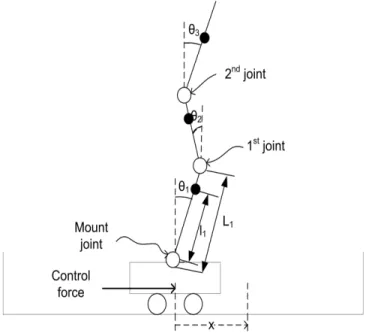
The three-network approach mentioned above is now tested on triple-link in-verted pendulum, which is unstable with multivariables and exhibits non-negligible nonlinearities. This kind of pendulum is frequently used to evaluate the perfor-mance of new control strategies. Here we consider the same system model as in [68]. Fig.3.4 shows a schematic diagram depicting the notations used.
Figure 3.4. Definition of notation used in the system equations for the triple link inverted pendulum benchmark
The nonlinear dynamic equations of this system can be expressed as: F(q)d 2q dt2 =−G(q, dq dt) dq dt −H(q) +L(q, u) (3.26) where F(q) =
A1 A2cos(θ1) A3cos(θ2) A4cos(θ3)
A9cos(θ1) A10 A11cos(θ1−θ2) A12cos(θ1−θ3)
A18cos(θ2) A19cos(θ1−θ2) A20 A21cos(θ2−θ3)
A28cos(θ3) A29cos(θ1−θ3) A30cos(θ2−θ3) A31
(3.27) G(q, dq dt) =
A5 A6sin(θ1) ˙θ1 A7sin(θ2) ˙θ2 A8sin(θ3) ˙θ3
0 A13 A14sin(θ1−θ2) ˙θ2+A15 A16sin(θ1−θ3) ˙θ3
0 A22sin(θ1−θ2) ˙θ2+A23 A24 A25sin(θ2−θ3) ˙θ3+A26
0 A33sin(θ1−θ3) ˙θ1 A35sin(θ2−θ3) ˙θ2+A36 A32 (3.28) q= x θ1 θ2 θ3 (3.29) H(q)= 0 A17sin(θ1) A27sin(θ2) A34sin(θ3) (3.30) L(q, u) = Ksu−sgn(x)µxA37 −sgn(θ1)µ1A38 −sgn(θ2)µ2A39 −sgn(θ3)µ3A40 (3.31)
Note that all the µhere is the Coulomb friction coefficient for links and is not
linearizable. In this simulation, µx = 0.07, µ1 = µ2 =µ3 = 0.003, and Ai are all
available in Table 3.3. The parameters in Table 3.3 are defined in the following:
L1 : 0.43m, total length of the 1st link;
L2 : 0.33m, total length of the 2nd link;
Table 3.3. System constants for the triple link inverted pendulum problem
Constant Value Constant Value
A1 M+m1+m2+m3 A2 m1l1+ (m2+m3)L1 A3 m2l2+m3L2 A4 m3l3 A5 Cc A6 −m1l1−(m2+m3)L1 A7 −(m2l2+m3L2) A8 −m3l3 A9 m1l1+ (m2+m3)L1 A10 I1+m2l21+ (m2+m3)L21 A11 (m2l2+m3L2)L1 A12 m3l3L1 A13 C1+C2 A14 (m2l2+m3L2)L1 A15 −C2 A16 m3l3L1 A17 −g(m1l1+m2L1+m3L1) A18 m2l2+m3L2 A19 (m2l2+m3L2)L1 A20 I2+m3L22+m2l22 A21 m3l3L2 A22 −(m2l2+m3L2)L1 A23 −C2 A24 C2+C3 A25 m3l3L2 A26 −C3 A27 −g(m2l2+m3L2) A28 m3l3 A29 m3l3L1 A30 m3l3L2 A31 I3+m3l23 A32 C3 A33 −m3l3L1 A34 −gm3l3 A35 −m3l3L2 A36 −C3 A37 1.3 A38 0.506 A39 0.219 A40 0.568
L3 : 0.13m, total length of the 3rd link;
l1 : 0.37m, length from mount joint to the center of gravity of 1st link;
l2 : 0.3m, length from 1st joint to the center of gravity of 2nd link;
l3 : 0.05m, length from 2nd joint to the center of gravity of 3rd link;
m1 : 0.4506kg, mass of the 1st link;
m2 : 0.219kg, mass of the 2nd link;
m3 : 0.0568kg, mass of the 3rd link;
M : 1.014kg, mass of the whole cart;
g : 9.8m/s2, acceleration of gravity;
I1 : 0.0042kgm2, mass moment of inertia of the 1st link about its center of
gravity;
I2 : 0.0012kgm2, mass moment of inertia of the 2nd link about its center of
gravity;
I3 : 0.00010609kgm2, mass moment of inertia of the 3ird link about its center
of gravity;
Cc : 5.5N ms, dynamic friction coefficient between the cart and the track;
C1 : 0.00026875N ms, dynamic friction coefficient for the 1st link;
C2 : 0.00026875N ms, dynamic friction coefficient for the 2nd link;
C3 : 0.00026875N ms, dynamic friction coefficient for the 3rd link;
In this case, the only control unit u (in voltage), generated by the action
network, is converted into force by an analog amplifier (with gain Ks = 24.7125
Newtons/volt) to the DC servo motor. Each link here only rotates in a vertical
plane, and the sample time interval is chosen to be 5ms. In order to better show the
performance of the proposed three network algorithm with Runge-Kutta methods,
the system equations are transformed into the state-space forms as follows: ˙ Q(t) = f (Q (t),u (t)) (3.32) f(Q(t),u(t)) = 04×4 I4×4 04×4 −F−1(Q(t))G(Q(t)) + 04×1 −F−1(Q(t))[H(Q(t))−L(Q(t),u(t))] (3.33) and Q= x θ1 θ2 θ3 x˙ θ˙1 θ˙2 θ˙3 (3.34) Specific physical meanings for these eight state variables are illustrated in the Fig.3.4. They are:
a)x, position of the cart on the track;
b)θ1, vertical angle of the 1st link joint to the cart; c)θ2, vertical angle of the 2nd link joint to the 1st link;
d)θ3, vertical angle of the 3rd link joint to the 2nd link;
e) ˙x, cart velocity;
f) ˙θ1, angular velocity of θ1; g) ˙θ2,angular velocity of θ2; h) ˙θ3, angular velocity of θ3.
Environment Setup
In this experimental setup, the constraints for the triple-linked inverted pen-dulum are: 1) The cart track extends 1.0 meter to both sides from the center
point; 2) The voltage applied to the motor should be within [−30,30]V; 3) Each
link angle should be within the range of [−20◦,20◦] with respect to the vertical axis.
Here, condition 2) is guaranteed by using a sigmoid function. While for the other two conditions, if either one fails or both fail, the system will be provided with an
all the time. Based on this external reinforcement signal, the three-network ADP approach will automatically and adaptively develop an internal reinforcement sig-nal to facilitate the learning and optimization process over time. For performance assessment, the same criteria as in [68] are adopted for this triple-linked inverted pendulum in this case study.
One hundred runs in this current study are conducted. Similarly as cart-pole problem, for different runs, here I will use different initial starting states. Specif-ically, I set the three angles and angle velocity of the triple links to be uniformly within the range of [−1◦,1◦] and [−0.50,0.50] ∗180/pi rad/s, respectively. As
for x and ˙x, their initial states are set to zero. The critic network is chosen as a
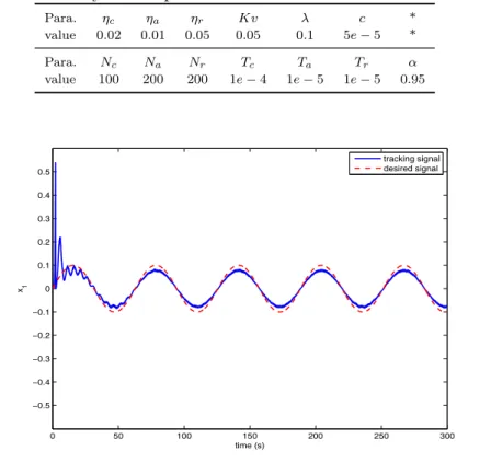
10-20-1 multi-layer perceptron (MLP) neural network structure [71, 72]. That is to say there are 10 input neurons, 20 hidden layer neurons, and 1 output neuron in this neural network. The action neural network is chosen as 8-14-1 MLP structure and the reference network is set as 9-14-1 MLP structure. The learning parameters such as learning rate, internal cycle, and internal training error threshold for the action network, reference network, and critic network are presented in Table 3.4. Table 3.4. Summary of the parameters used in triple-link inverted pendulum bal-ancing task Para. lc(0) la(0) lr(0) lc(f) la(f) lr(f) * value 0.3 0.3 0.3 0.001 0.001 0.001 * Para. Nc Na Nr Tc Ta Tr α value 80 100 50 0.05 0.005 0.05 0.95 Simulation Analysis
Summary of the simulation results with different noise conditions are presented in Table 3.5. Comparing with those in [68], the proposed three-network ADP architecture can achieve competitive results in this case as well. To observe how the proposed approach performs under this task, here I present a snapshot of the
0 10 20 30 40 50 60 70 80 90 100 0 500 1000 1500 2000 2500 3000 Run number number of trials (a) 0 500 1000 1500 2000 2500 3000 0 2 4 6 8 10 12 14 16 18 20
Histogram of number of trials in successful runs
number of trials in successful runs (b)
Figure 3.5. Statistics of the successful runs. (a) Number of required trials for the successful runs. (b) Histogram the statistics.
statistics of different runs under noise free condition. Fig. 3.5(a) shows the number of required trials for each successful run, and Fig. 3.5(b) shows the corresponding histogram information. The three angles and angle velocities of the triple links are set to be uniformly within the range of [−1◦,1◦] and [−0.50,0.50]∗180/pi rad/s,
respectively, and the initial states of x and ˙x are set to zero.
Table 3.5. Performance evaluation on case II: triple-link balancing task. The 2nd and the 3rd columns are with our proposed method, while the 4th and the 5th columns are the results from existing approach
Noise type Success rate ] of trial Success rate ]of trial
Noise free 99 % 571.4 97 % 1194 Uniform 5% a. 99 % 596.9 92 % 1239 Uniform 10% a. 99 % 673.1 84 % 1852 Uniform 5% s. 99 % 620.1 89 % 1317 Uniform 10% s. 99 % 657.9 80 % 1712 Gaussian σ2(0.1) s. 80 % 1170.4 85 % 1508 Gaussian σ2(0.2) s. 50 % 1372.2 76 % 1993
To further analyze how the proposed ADP structure can accomplish the con-trol task, Fig. 3.6(a) to 3.6(h) show a typical trajectory on the task for all the
0 1000 2000 3000 4000 5000 6000 −0.015 −0.01 −0.005 0 0.005 0.01 0.015 0.02 x Time Step x(m) (a) 0 1000 2000 3000 4000 5000 6000 −0.02 −0.015 −0.01 −0.005 0 0.005 0.01 0.015 0.02 Time Step Theta 1 (rad) Theta 1 (b) 0 1000 2000 3000 4000 5000 6000 −0.01 −0.005 0 0.005 0.01 0.015 Time Step Theta 2 (rad) Theta 2 (c) 0 1000 2000 3000 4000 5000 6000 −10 −8 −6 −4 −2 0 2 4 6 8x 10 −3 Time Step Theta 3 (rad) Theta 3 (d) 0 1000 2000 3000 4000 5000 6000 −0.08 −0.06 −0.04 −0.02 0 0.02 0.04 0.06 0.08 0.1 Time Step x Dot(m/s)
The velocity of the cart
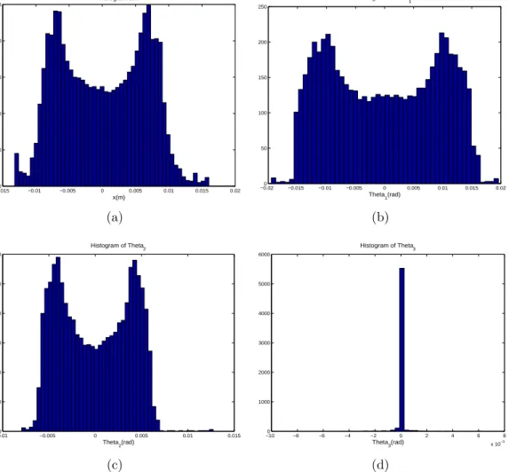
(e) 0 1000 2000 3000 4000 5000 6000 −0.4 −0.3 −0.2 −0.1 0 0.1 0.2 0.3 Time Step Theta 1 Dot(rad/s) Theta 1 Dot (f) 0 1000 2000 3000 4000 5000 6000 −0.15 −0.1 −0.05 0 0.05 0.1 Time Step Theta 2 Dot(rad/s) Theta2 Dot (g) 0 1000 2000 3000 4000 5000 6000 −0.4 −0.3 −0.2 −0.1 0 0.1 0.2 0.3 0.4 Time Step Theta 3 Dot(rad/s) Theta3 Dot (h)
Figure 3.6. Typical trajectory on the triple-link inverted pendulum balancing task. (a) The position x of the cart. (b) The 1st joint angle of the triple link pendulum. (c) The 2st joint angle of the triple link pendulum. (d) The 3st joint angle of the triple link pendulum. (e) The velocity of the cart. (b) The angular velocity of the 1st joint angle of the triple link pendulum. (c) The angular velocity of the 2st joint angle of the triple link pendulum. (d) The angular velocity of the 3st joint
−0.0150 −0.01 −0.005 0 0.005 0.01 0.015 0.02 50 100 150 200 250 x(m) Histogram of x (a) −0.020 −0.015 −0.01 −0.005 0 0.005 0.01 0.015 0.02 50 100 150 200 250 Theta1(rad) Histogram of theta1 (b) −0.010 −0.005 0 0.005 0.01 0.015 50 100 150 200 250 300 Theta 2(rad) Histogram of Theta 2 (c) −10 −8 −6 −4 −2 0 2 4 6 8 x 10⁻³ 0 1000 2000 3000 4000 5000 6000 Histogram of Theta 3 Theta 3(rad) (d)
Figure 3.7. Typical histogram on the triple-link inverted pendulum balancing task. (a) The histogram of position x of the cart. (b) The histogram of the 1st joint angle of the triple link pendulum. (c) The histogram of the 2st joint angle of the triple link pendulum. (d) The histogram of the 3st joint angle of the triple link pendulum.
state variables under noise free condition, namely the the position x of the cart
(3.6(a)), the first, second, and third joint angle of the triple link pendulum (3.6(b) to 3.6(d)), the velocity of the cart 3.6(e), and the angular velocity of the first, second, and third joint angle of the triple link pendulum (3.6(f) to 3.6(h)). The
corresponding histogram information for the position x and three joint angle
in-formation are also shown in Fig. 3.7(a) to Fig. 3.7(d). All these results clearly indicate that the proposed ADP approach can effectively control the system to achieve desired states during the online learning process.
0 1000 2000 3000 4000 5000 6000 −0.15 −0.1 −0.05 0 0.05 0.1 0.15 0.2 0.25 Time Step J (a) (b)
Figure 3.8. Typical trajectory of cost-to-go and control action signal on the triple-link inverted pendulum balancing task. (a) The cost-to-go signal on the task. (b) The control action signal on the task.
an internal reinforcement signal to facilitate the learning and optimization in the
ADP structure, I further analyze how the J value and control action u looks like
in this case. Fig. 3.8(a) shows a snapshot of the convergence of theJ value during
the learning process, and Fig. 3.8(b) shows another snapshot of the control action
u during a typical successful run. Both figures also clearly demonstrate that our
proposed approach can effectively accomplish the control performance in this case.
3.5 Summary
A three-network ADP architecture with an action network, a critic network, and a reference network, for adaptive learning, control, and optimization is pre-sented here. The key idea of this approach is the introduction of a new reference network (will be called goal network in the remaining of this dissertation) to de-velop internal goal-representation to facilitate learning and optimization. It pro-vides an effective way to adaptively and automatically build the internal goal rep-resentations for the intelligent systems. A detailed design architecture and learning algorithm is presented, followed by detailed simulation analysis on two benchmark tasks (i.e., balancing a cart-pole model and a triple-link inverted pendulum model) to demonstrate the effectiveness of our approach. In the next chapter, I am go-ing to further demonstrate its adaptive learngo-ing mechanism in an trackgo-ing control problem.
CHAPTER 4
Goal Representation Design for Heuristic Dynamic Programming (GrHDP) Architecture
4.1 Introduction
A “Dual” critic network technique is integrated into the ADP architecture, and this new architecture is called goal representation heuristic dynamic programming (GrHDP) design [73, 74]. Specifically, an alternative choice rather than crafting the reinforcement signal manually from priori knowledge is proposed. The overall adaptive learning performance has been tested on two tracking control benchmarks with a tracking filter. For comparative studies, the tracking performance with the typical HDP is also presented to justify the improved performance. Furthermore, a virtual reality (VR) platform is provided to demonstrate the real-time simula-tion under different disturbance situasimula-tions. Detailed Lyapunov stability analysis for the proposed approach is presented to support the proposed structure from a theoretical point of view (see Appendix A).
4.2 Design of GrHDP for Tracking Control
The schematic diagram of this proposed idea is presented in Fig.4.1. The action network is kept the same as that in [68, 51]. While for the critic network, I integrate with one reference network (also called goal network) and therefore there are two networks in the dual-critic network block as presented in Fig.4.2. The tracking filter is added to show the performance on tracking control problem. The following of this section will introduce the dual critic network block and the tracking filter, respectively.