Maximum entropy and learning theory

Maximum

Entropy

and

Learning Theory

Griff

L.

Bilbro

Center for Communications

and

Signal Processing

Department of Electrical

and

Computer Engineering

North Carolina State University

Maximum Entropy and Learning Theory

Griff L. Bilbro

David E. Van den Bout

North Carolina State University, Box

7914

Raleigh, NC 27695-7914

March

22, 1991

Abstract

We derive the learning theory recently reported by Tishby, Levin, and Solla (TLS) without statistical mechanics. We show that the theory generally applies to any problem of modeling data. We analyze an elementary example for which we find the predictions consistent with intuition and conventional statistical results. We numerically examine the more realistic problem of training a competitive net to learn a one dimensional probability density from samples. We find TLS useful for predicting average training behavior.

1

Introduction

A statistical theory which describes the learning of a relation from examples was reported in (Tishby, Levin, and Solla, 1989). It built on earlier work in (Schwartz, Samalan, Solla, and Denker, 1990)and has been carefully restated in (Levin, Tishby, and Solla, 1990). In that literature, statistical mechanics was used to relate the probability of independent input-output data pairs to a layered neural network.

2

Maximum entropy and modeling

In this section we will show that a TLS theory can be constructed for any problem in which parameters of a model are chosen to fit data. Consider a problem in which data _{xi}~~f drawn from an unknown density p(x) are to be fitted with some model by adjusting parameters w to minimize an additive error function during a training procedure. In the case of training a layered feedforward net, the data are input-output pairs; the parameters w

are the usual weights and biases; the error function and training procedure might be squared error and backpropagation. However the theory is much more general. In later sections, we will apply it to the simplest case of linear regression and to the case of learning a one dimensional probability density. Except for the case of linear regression, there is little theoretical guidance for identifying when data is sufficient to determine the model. Often the total set of available data {xi}~~fis divided into a training set {Zi}~~~ and a re-maining test set. The model is trained to a specified error er on {Xi}:~~ and then tested against the remaining data. In principle this procedure could be repeated for randomly selected test sets and initial values and the av-erage results could be tabulated as functions of m and er- Implicit in this hypothetical exercise is an average density (p(m)(

w))z

of nets trained to an error er on m examples. The true (p(m)(w))z would be difficult to calculate

in general, mostly because it involves the details of the training procedure. However the end result of training may depend more on the form of the model, the amount of the data, the noise in the data, and the training error

f.T, than on the details of the training procedure. In that case, the

maxi-mum entropy density (p(m)(w))z resembles (p(rn) (w))z and might be used to predict training behavior and generalization.

The principle ofmaximum entropy is a general inference tool which pro-duces probabilities characterized by certain average values of specified func-tions(Jaynes, 1979). To the extent that entropy measures information, a maximum entropy estimate contains only the information implied by those average values and makes no other assumptions

(e.g.

about the training pro-cedure). It is useful to also incorporate a prior estimate p(O)(w) ofp(m)(w) by considering the entropy of p(m)(w) relative to p(O)(w)

In our practice so little is known about p(m)(w) that p(O)(w) is chosen merely as a restriction to reasonable portions of w space. For example, in back propagation it is unreasonable to expect the weights as large as 0(106 ) and perhaps 0(1) is a little too small. In any case the first test of this theory must be for sensitivity to p(O)(w) .

In the maximum entropy sense, the density p(m)(w) that contains the least information beyond p(O)(w) but is nevertheless a normalized density with integral

f

dwp(m)(w)

=

1

and with specific average training error

(2)

can be found with calculus of variations and two Lagrange multipliers Q and

(3 in the usual way. The extremum satistifies

(4)

which can be solved for p(m)(w) to get

(5)

where (3 has been left, but expll - a) has been evaluated in terms of the more conventional normalization

(6)

that depends on the particular set of examples as well as their number. Equation 5 is significant. It is an estimate of the probability density of models of the form (i.e. architecture for a neural net) defined by the func-tional relation between wand x in

f(

X,w) after being trained from random

initial values of w to an average error Equation 3 on the particular data set

set {Xi}~~;n

.

In order to remove that effect, we average Equation 5 over all possible m examples

(7)

Equation 7 can be used to define a performance criterion, the average

prediction fraction

</J(m)

=

f

dw

f

_{dXm+1P(xm+dexp(-,Bf(X m+b W))(p(m)(w)):I:} (8)

which is the fraction of models distributed according to p(m)(w) which have an error function f within about

1/

f3 of the next unseen example X m+l on

average.

Equations 7 and 8 are inconvenient to evaluate exactly because of the

z(m) term of Equation 6 in their denominators. TLS propose an "annealed approximation" which in the present context is equivalent to replacingz(m) in Equation 7 by its average over ways of choosing {Xi}~~r

(z(m) ):1:

=

f

dw

f

dx(m)p( xdp( X2)"·P( xm)p(O)(w) exp(

-,BL~~~

f(

Xi, w) )

(9)

which can be written

(10)

where

f(w)

=

f

dxp(x)exp(-,Bf(X,W)).

(11)

With this the average prediction fraction of Equation 8 becomes

Equation 12 predicts generalization behavior by drawing a maximum entropy inference of the average consistency between the model represented by f(X,w)

and m examples drawn from p(x).

2.1

Relation to

TLS

In this subsection we will show that under the assumptions of Tishby, Levin, and Solla, our average predition fraction is proportional to their Average Prediction Probability ((p(m)))

where

4J(m)

==

z({3)( (p(m))) ₍₁₃₎

z(l1)

= /

dxexp(-l1e(x,w)) (14)

normalizes the probability density for the conditional probability

1

p(xlw) - z(l1) exp(-l1e(x,w)) (15)

which TLS use to describe the behavior of a single certain netw. Equation 15 can itself be obtained from a maximum entropy argument in z space but we will not do so here.

Now z is a function of

(3

but is assumed in TLS to be independent of w. TLS show this to be rigorously true for layered nets with real outputs if € is the usual squared error between data and output. It is true in that

case because the area under a Gaussian is independent of the mean of the Gaussian.

OUf derivation here is more direct than existing derivations of TLS, who

apply Bayes' rule to statistical mechanics. In their treatment, the extra factor of z appears naturally. We can demonstrate the equivalence Equation 13 as follows. We solve Equation 15 for the exponential and substitute it into Equation 11

f(w)

= /

dxp(x) z(l1)p(xlw)

=

z(l1)g(w) (16)

where

g(w)

was defined as "the average generalization of the network" in (Tishby, Levin, Solla, 1989) "the sample average of the likelihood" of the network (Levin, Tishby, Sella, 1990) to be

g(w)

= /

dxp(x)p(xlw). (17)

We now substitute this into Equation 12 to get

zm+l

((3)

J

dwp(O)(

w

)grn+l

(w)

(19)

which yields Equation 13 since Levin, Tishby, and Solla define APP as

( m+l)

((p(m»))

=

"Y p(O)

(,m)

p(O)

where we have used, to distinguish their va.rable9 from the function g(w).

They define the denominator of this expression as

(20)

which can be evaluated with the Dirac delta function to get

(21)

(22)

with a similar expression for the numerator, so that

((p(m»)) _ Jdwp(O)(w)gm+l(w)

_-

_J

dwp(O)( w

)gm(

w) .

Equation 13 follows immediately from Equations 22 and 12. Therefore our average prediction fraction is identical (except for a scale factor

z(,B))

to the TLS average prediction probability under the conditions that TLS assume.

For some problems we could argue that our </J(m) is a more natural

per-formance measure than the TLS ((p(m»)) . But in fact, the two are identical except for scale

z((3)

and the TLS restriction on the w dependence of that scale. For consistency with the existing work of Tishby, Levin, and Solla, we will use their ((p(m»)) in the remainder of this report.

3

Analysis of an elementary example

We take the true value of the constant to be wand assume the noise to be zero mean additive Gaussian of variance 1/20., so that the density of a measurement with value x is

(24)

We choose a simple prior density as a Gaussian with mean Wo and variance

1/2r

p(O)(w)

=

~e-"(W-Wo)2.

We choose the simplest error function

(25)

(26)

the squared error between a sample :v and the our estimate w.

According to TLS we now analyze the problem. We substitute the error function into Equation 15 to get

p(zlw)

== _1_

_e-

13(:c - w )2

z({3)

(27)

with z(;3)

=

~ which is independent of w as assumed. We determine {3 by

solving

(28)

(29)

to get

1

{3

== - .

2fT

The generalization, Equation 17, can now be evaluated with Equation 23

where

0.{3

K

=

a

+

{3'

(31)

is less than either a or (3. The denominator of Equation 22 becomes

It /

~

rnnr

( ) 2 )

(

)

( _)m 2 exp ( -

w -

Wo 32

11" r

+

mit mlt+r

3.1

Large training set size

TIle case of many examples or little prior knowledge is interesting. Consider Equations 22 and 32 for ni«

> >

r

(33)

which climbs to an asymptotic value of

fi

for m ~ 00. In order to

compare this with intuition, consider that the sample mean of

{Xl,

X2, ... ,xm }

approaches w to within a variance of 1/2ma, so that

(34)

which makes Equation 22 agree with Equation 33 for large enough {3. In this sense, the statistical mechanical theory of learning differs from conventional Bayesian estimation only in its choice of an unconventional performance cri-terion APP.

3.2

Small training set size

We can demonstrate overtraining even for this elementary example when the size of the training set m is small and the the error on the training set er is

reduced too much. It will be sufficient to consider Equation 12 for m«

<<

r

so that

(35)

by which Equation 22 becomes

(36)

This expression for APP depends on '" which in turn depends on {3 which is finally determined by the training target error fT. As a function of «,

Equation 36 exhibits a maximum at

1 "'opt=: ·

Using Equations 29 and 31, we find that the system will have the highest average prediction probability if training is stopped when the error on the training set is

(

-)2

1

€T,opt

=

Wo - W - 20: (38)

which depends only on the variance of the target distribution 1/20. and the difference between the mean of the prior distribution Wo and the mean of the

target distribution w. Since

(f)

and er cannot be negative, this optimum is physical only when it is positive. So when Equation 38 is negative, training should continue to the smallest possible error, since in that case there is no danger of overtraining. Now fT,opt

>

0 occurs only when the error of the

prior estimate for the unknown constant is larger than the width of the prior distribution. Furthermore it can occur only when m is not too large, since we have assumed m«

«T.

We can therefore translate Equation 38 into the following rule for this simplest of systems: overtraining occurs when the system is trained to too Iowan error (i.e. er

<

fT,opt) on a training set that

is too small (i.e. m

<

<

TK)

to compensate for an initial overconfidence in the prior estimate

(i.e.

2~

> (wo -

w)2).

4

General numerical procedure

In this section we show how to numerically apply the theory. We can estimate the moments of Equation 22 by the following Monte Carlo procedure. Given a data set {xi}:~fdrawn from the unknown density p on domain X with finite volume V, an error function

f(zlw),

a training error fT, and a prior

density p(O)(

w)

of vectors such that each

w

specifies a candidate model,

1. Construct two sample sets: a prior set of Np functions

{wp}

drawn from

p(O)(

w)

and a set of Nu input vectors

{xu}

drawn uniformly from X. For

each p in the prior set and every u in the uniform set, tabulate the error

fup

==

f(zulwp).

For each i in the training set and every u in uniform set tabulate

fip

==

f(Xilwp).

2. Determine the sensitivity(3 for a specified er by solving

'"'" e-{3£upe

LJu

up

- - - = = fT·

L:u

e -f3£up

Equation 39 can be shown to be monotonic in f3 so this involves a simple one-dimensional search.

3. Estimate the average generalization of a given Wp from Equation 17

1 1/N

Ei

e-{3£ip

g(

wp

)

=

V

1/

N_u

Eu

e-{3€.." •

(40)

The factor of V remains in this particular expression because each proba-bility density is normalized to have unit integral over X so that the Monte Carlo expression for integral of their product retains one factor of V, the integral of X itself.

4. The performance after m examples is the ratio of Equation 22.

By

con-struction the W_p are drawn from p(O)(w) so that

(41)

5

Learning a density

A TLS theory is completely specified by a dataset {~i}~~f (or the corre-sponding density

p(

~) in pattern or data space), a prior density p(O)(w) in

w space, and an error function f(X,W) that relates x's to w's. In this sense, learning a density is no different from learning a map. The error function

f(

e ,w) measures some important difference between data and model and for learning a density, the negative of the log likelihood is a natural choice.

,

~

'.

•

•

~

•

•

•

•

_•

•• •

_•

•• • •• • ••

J

J

~

w2

0 0_e

0

0 0_{o 0} e

0." 0

e E)."0 000 ~o

of)o go

0°_{e 0}

0°_{o 0} e 0.0 0

000 go

e 0.0 0

eCo go

0°

Of) o 0

e 0 _{e d'o0}

o 0.0 0 _{000 SO} 000 :C

w1

Figure 1: A 2 dimensional competitive learning net: topEvolution of neuron locations toward samples. bottom Equilibrium neuron locations in regions of high sample density.

Competitive learning nets with conscience qualitatively change their be-havior when they are trained on finite sample sets containing fewer examples than neurons; except for that regime we found the theory satisfactory.

A CLN with k neurons is specified by a vector w of k neuron locations. We restricted ourselves to a one-dimensional problem on the unit interval. All experiments we will present in this section were conducted upon data drawn from the following one-dimensional training density

_ x

== {

2VFz

0

<

X

<

1,

p()

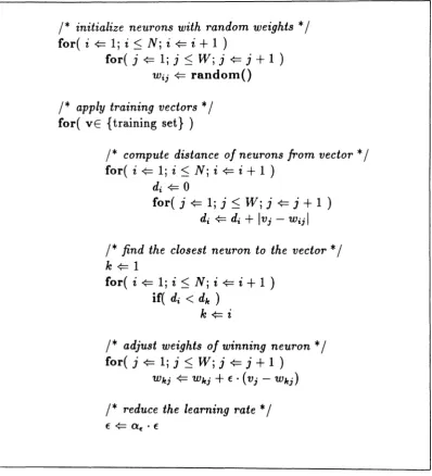
0 otherwise.

/*

initialize neurons with random weights

*/

for( i ¢:: 1;i

:s;

N; i {= i

+

1 )

for( j {= 1;j:::; W; j ¢:: j

+

1 )

Wij ¢:: random()

/*

apply training vectors

*/

for( vE {training set} )

/*

compute distance of neurons from vector

*/

for(

i

¢:: 1;

i:S

N; i {= i

+

1 )

di ¢:: 0

for( j {= 1;

j:S

W; j {= j

+

1 )

d, ¢:: d;

+

IVj - wijl

/*

find the closest neuron to the vector

*/

k{=1

for( i {= 1;i

:S

N; i ~ i

+

1 )

if( di

<

die )

k¢=i

/*

adjust weights of winning neuron

*/

for( j ¢= 1;j

:S

W; j ~ j

+

1 )

Wlej ¢= Wlej

+

f · (Vj - w/ej)

/*

reduce the learning rate

*/

f {= Q£ • f

of prior densities. We chose the error function

i=k

f{X,W) == min Ix - Wil

1=1 (42)

which is the distance between the sample x and location of the nearest neuron

uu, The error of several samples is the sum of the separate errors. If the samples are assumed to be independently drawn so that the joint probability of a set of samples is the product of the component probabilities, it can be shown that € is proportional to the log of the conditional probability of

observing x given the CLN w. Our chosen form for f therefore corresponds

to an exponential density around each neuron

(43)

for x close enough to the it h _{neuron. The neurons of a trained CLN tend to} cluster in regions where the data density is highest. For m ~ k ~ 1, the distribution of neurons can be represented by a density which approaches a power the density of the data (Ritter, 1991).

In Figure 3 is the Average Prediction Probability (APP) for k == 20 versus

m, for several values of target error

er

and for two prior densitsities; first consider predictions from the uniform prior. For

er

== 0.01, APP practically attains its asymptote of 1.5 by m == 40 examples. Assuming the APP to be dominated in the limit by the largest 9, we expect a CLN trained to an error of 0.01 on a set of 40 examples to perform 1.5 times better than an untrained net on unseen samples drawn from the same probability density. We can therefore define a predicted probable error of order

1

€",.ob

=

2 k p(m) · (44)

For k

==

20, fprob

==

0.017 for

er

==

.01 and fprob

==

0.021 for

er

== 0.02.

100 20 40 eo 80

Trainingset81ze

2 . . . - -...----.11..---.--...- - . . ,

0.7 ~ -...---.l~-

...- ...- -...

o

100 20 40 eo 80

Training Set Size

2..--...----...--...- ...---,

0.7 ""--_..._ - - - 1 0_ _. . 1 0 . - _. . . . ._ - "

o

1.5 .010 1.5

.013

015 .010

.011 :SIi

.01f' :8lb

,

.021 t

C

(a)

(b)

0.04

r---..---.----_

_{0.04 r----~---...----_}

0.03

(b)

0.01 0.02 TNlnlng ErTor

0 . 0 1 - - - & - - -...- - -....

o

0.03

(a)

0.01 0.02 TNlnlng Error

0.01---...- - -...- - - '

o

0.03 0

0.03

..

-

0 0

!

t.

.

_•

o(

.

_!

I

J

~

0.02 _0.02

Figure 4: Experimentally determined and predicted values of total error across the training density after competitive learning was performed using a 20-neuron network trained to various target errors (a) with 40 samples, (b)

with 20 samples.

of APPs for m

==

20 and m

==

40. For the case of m

==

20 examples, the same net can only be expected to exhibit probable errors of .019 and .023 for corresponding training target errors, which is compared graphically in Figure 4 with the experimentally determined errors for m

==

20.

The APP curves saturate at a value of m that is insensitive to the prior density from which the nets are drawn. The vertical scale does depend some-what on the prior however. Consider Figure 3, which also shows the APP curves for the same k

==

20 net with the prior density antisymmetrically skewed away from the true density by the following function:

(0) w

== {

2J~-w

0::; w

<

1,

p ( ) 0 otherwise.

because in actual training, the effect of the initial configuration is also quickly lost. For m

<

20 the predictions are not valid in any case, since our simple error function does not reflect the actual probability even approximately for

m

<

k in these nets. It is for m

<

20 where the only significant differences

between the two families of curves occur. We have also been able to draw the same conclusions from less structured prior densities generated by assigning positive normalized random numbers to intervals of the domain. In fact, we were not able to produce curves worse than those of Figure 3.

Moreover, we generally find that TLS predicts that about twice as many samples as neurons are needed to train competitive nets of other sizes.

The previous curves were produced with large total sample sets N = 1000. We subsequently reran the experiments with N

=

100 with essentially iden-tical results (we do not plot them because the two are indistinguishable). It is reassuring that the predictions of the theory are reliable even for relatively small sample sets.

6

Conclusion

We have derived the TLS theory of learning using the principle of maximum entropy instead of a combination of statistical mechanics and Bayes' rule. We show that TLS can be applied generally to learning and modeling. We apply it to learning a constant and to learning a one dimensional density in the annealed approximation of TLS. We considered the effects of varying the number of examples m, the target training error fT (or equivalently

{3),

and

the choice of prior density p(O)(w) . These experiments on learning a density are consistent with learning a binary output (Bilbro and Snyder, 1990), a ternary output (Chow, Bilbro, and Yee, 1990), and a continuous output (Bil-bro and Klenin, 1990). We find if saturation occurs for m substantially less than the total number of available samples, say m

<

T/2, that m is a good predictor of sufficient training set size. Moreover there is evidence from a reformulation of the learning theory based on the grand canonical ensemble that also supports this statistical approach (Klenin,1990). For small prob-lems the theory is very easy to use. We have no experience yet in applying the theory to large problems with say more than 50 unknown weights or parameters.

set size, however another question remains. It is difficult to obtain large overtraining effects from this theory even though some traces of overtraining remain: The curves of Figure 3 can be made to cross for small m and poor prior. In the Equation 38 of the elementary example, it is possible to obtain a positive fT,opt. However it appears that some aspects of overtraining do not

survive the annealed approximation. This is consistent with the experience of other workers(Solla, 1990).

References

G. L. Bilbro and M. Klenin. (1990) Thermodynamic Models of Learning: Applications. Unpublished.

G. L. Bilbro and W. E. Snyder. (1990) Learning theory, linear separabil-ity, and noisy data. CCSP- TR-90/7, Center for Communications and Signal Processing, Box 7914, Raleigh, NO27695-7914.

M. Y. Chow, G. L. Bilbro and S. O. Vee. (1990) Application of Learning Theory to Single-Phase Induction Motor Incipient Fault Detection Artificial Neural Networks. Submitted to International Journal

0/

Neural Systems.

D. DeSieno. (1988) Adding a conscience to competitive learning. In IEEE

International Conference on Neural Networks, pages 1:117-1:124.

E. T.

Jaynes. (1979) Where Do We Stand on Maximum Entropy? In R. D. Leven and M. Tribus (Eds.), Maximum Entropy Formalism, M. I. T. Press, Cambridge, pages 17-118.

M. Klenin. (1990) Learning Models and Thermostatistics: A Descrip-tion of Overtraining and GeneralizaDescrip-tion Capacities. NETR-90/3, Center for Communications and Signal Processing, Neural Engineering Group, Box 7914, Raleigh, NC 27695-7914.

E. Levin, N. Tishby, and

S. A.

Solla. (1990) A Statistical approach to learning and generalization in layered neural networks. Proceedings of the

IEEE,

Vol. 78, No. 10, pages 1568-1574.

D. B. Schwartz, V. K. Samalan, S. A. Solla &

J.

S. Denker. (1990) Exhaustive Learning. Neural Computation.

H. Ritter. (1991) Asymptotic Level Density for a Class of Vector Quan-tization Processes. IEEE Trans. NN.

D. Rumelhart and J. McClelland. (1986) Parallel Distributed Processing:

Ezploraiions in the Microstructure of Cognition, Chapter 5, MIT Press.

N. Tishby, E. Levin, and S. A. Solla. (1989) Consistent inference of probabilities in layered networks: Predictions and generalization.

IJCNN,

IEEE, New York, pages 11:403-410.

D. E. Van den Bout and T. K. Miller III. (1990) TInMANN: The integer Markovian artificial neural network. Accepted for publication in the Journal