Isolated and Ensemble Audio Preprocessing Methods for Detecting
Adversarial Examples against Automatic Speech Recognition
Krishan Rajaratnam 1, Kunal Shah 2, Jugal Kalita 3
1 The College, University of Chicago, Chicago, USA
2 College of Liberal Arts and Sciences, University of Florida, Gainesville, USA
3 Department of Computer Science, University of Colorado, Colorado Springs, USA
1 [email protected], 2 [email protected], 3 [email protected]
Abstract
An adversarial attack is an exploitative process in which minute alterations are made to
natural inputs, causing the inputs to be misclassified by neural models. In the field of speech
recognition, this has become an issue of increasing significance. Although adversarial attacks
were originally introduced in computer vision, they have since infiltrated the realm of speech
recognition. In 2017, a genetic attack was shown to be quite potent against the Speech
Commands Model. Limited-vocabulary speech classifiers, such as the Speech Commands
Model, are used in a variety of applications, particularly in telephony; as such, adversarial
examples produced by this attack pose as a major security threat. This paper explores various
methods of detecting these adversarial examples with combinations of audio preprocessing.
One particular combined defense incorporating compressions, speech coding, filtering, and
audio panning was shown to be quite effective against the attack on the Speech Commands
Model, detecting audio adversarial examples with 93.5% precision and 91.2% recall.
Keywords: adversarial attack, speech recognition, deep learning, audio compression, speech coding
1. Introduction
Due to the widespread and growing use of neural networks for various tasks, it is imperative
that these models be robust and secure while remaining generally usable. Although these
models are quite powerful and are well-suited for a variety of tasks, they are not without their
imperfections. First applied against computer vision models [1], adversarial attacks exploit
the flaws of neural networks by making perceptibly insignificant changes to a source to
produce adversarial examples, with the purpose of causing the neural network to misclassify
the example. These attacks can be quite potent and have caused misclassification rates of
The 2018 Conference on Computational Linguistics and Speech Processing ROCLING 2018, pp. 16-30
above 90% in image classifiers [2]. Because of their exploitative nature, adversarial attacks
can be quite difficult to defend against without sacrificing general model usability or
accuracy.
The use of adversarial attacks is not restricted to the field of image recognition. Modern
speech recognition has become increasingly reliant on end-to-end neural models, which are
able to largely outperform traditional models that rely heavily on signal processing and
hidden Markov models. These sophisticated neural models may be state-of-the art, but are
also more susceptible to attack by adversarial examples. Recent work has shown that two
speech recognition models, a convolutional neural network (CNN) model trained on the
Speech Commands dataset [3] and Mozilla’s implementation of the DeepSpeech end-to-end
model [4], are vulnerable to adversarial attacks. Two separate attacks on the two models were
able to generate extremely potent adversarial examples, capable of inducing a
misclassification rate of up to 100%. This trend threatens the current reliability of deep
learning models within the field of speech recognition. As such, there is a crucial need for
defensive methods that can be employed to evade audio adversarial attacks.
2. Related Work
The attack against the limited-vocabulary Speech Commands model detailed by Alzantot et
al. [3] shows particular relevance within the field of telephony, as it could be applied to
maliciously manipulate the limited-vocabulary speech classifiers used for automated
attendants. During this attack, adversarial examples created by a gradient-free genetic
algorithm allow the attack to penetrate layers of non-differential preprocessing, which is
commonly used in automatic speech recognition.
2.1 Audio Preprocessing Defenses
Recent work in computer vision has shown that preprocessing methods, such as JPEG and
JPEG2000 image compression [5], resizing [6], and pixel deflection [7] are capable of
defending against adversarial attacks with varying degrees of success. Preprocessing defenses
have also been employed in speech recognition to mitigate adversarial examples. Yang et al.
[8] achieved a high rate of success with the use of local smoothing, down sampling, and
quantization in an attempt to neutralize adversarial examples produced by the attack of
(i.e. retrieving the original label of) 63.8% of the adversarial examples. Quantization causes
various amplitudes of sampled data to be rounded to the nearest integer multiple of the q
value; this allows adversarial perturbations with small amplitudes to become disrupted.
Work has also been done in employing audio compression, Hertz shifting, noise reduction,
and low-pass filtering [9], to defend against Carlini and Wagner’s attack [4] on DeepSpeech.
The results of [9] suggest that the most promising preprocessing method was low-pass
filtering, with which the authors were able to retrieve the original label of 90.11% of Carlini
and Wagner’s adversarial examples. By utilizing low-pass filtering, a selected range of higher
frequencies are eliminated, preserving a lower band of frequencies in which human speech is
located. If a significant portion of the of the adversarial perturbation is found within the
discarded higher frequencies, the attack can be disrupted. Although this work was able to
largely neutralize the threat of adversarial examples against DeepSpeech, this came at a
noticeable cost to general model accuracy.
2.2 Speech Coding
Although the results of [9] imply that low-pass filtering outclasses audio compression as a
preprocessing defense, this work only explored two standards of audio coding: Advanced
Audio Coding (AAC) and MP3. Though those two compression standards enjoy widespread
popularity, they are not necessarily adequately equipped in defending against targeted
adversarial examples on speech recognition. For the purposes of teleconferencing and VoIP,
speech codecs such as Speex [10] and Opus [11] are primarily used due to their ability to
preserve the quality of human speech, even through imperfect conditions and lower bitrates.
In 2002, Valin [10] began the Speex project with intent on providing “a free codec for free
speech.” Further development allowed Speex to grow in popularity, becoming adopted by
well-known, practical VoIP applications such as TeamSpeak and Twinkle . Speex codec is 1 2
built upon the Code Excited Linear Prediction (CELP) algorithm [12], which models the
vocal tract using a linear prediction model capable of minimizing differences of the
uncompressed source within a “perceptually weighted domain.” The minimization is
achieved by applying the following weighting filter to the raw input:
1 http://teamspeak.com/en/features/overview
where Ais a linear prediction filter with γ 1and γ2managing the filter shape. This filter allows
for various levels of noise at different frequencies and has proven to be useful for neutralizing
adversarial perturbations whilst maintaining the quality of human speech. In addition, Speex
also includes numerous features, such as voice activity detection, denoising, and support of
various bandwidths. As this compression seems to resemble audio preprocessing methods
proven capable of effectively mitigating adversarial examples, it seems better suited than
MP3 or AAC compression for the task of defending against adversarial attacks.
The Opus codec, which is used by the highly popular proprietary VoIP application Discord , 3
is a modern successor to the Speex codec [11]. By combining the CELP algorithm with
SILK, a linear predictive coding algorithm developed by Skype Technologies in 2009 , it is 4
considered an improved and more advanced version of Speex; the application of Opus
compression for defending against adversarial examples is therefore worth testing.
2.3 Ensemble Detection
Preprocessing defenses against adversarial examples can only be effective and practical if
they are able to mitigate adversarial examples without greatly compromising general model
accuracy. A viable form of preprocessing would disrupt the predictions of adversarial
examples more than it would disrupt the predictions of benign examples. In particular, there
should ideally be a small difference between the output vectors produced by passing the raw
input and preprocessed input through a neural network when the input is benign, but that
same difference should be much larger if the input is adversarial. This core idea can be used
to apply preprocessing methods to detect adversarial examples, rather than simply mitigating
or neutralizing perturbations.
Within the field of computer vision, ensembles of preprocessing methods have been used for
detecting adversarial examples. Xu et al. [13] proposed the feature squeezing method for
detecting adversarial examples. This method combines smaller “squeezing” methods into an
ensemble, and calculates an L1 score from of the maximum L1distance between any pair of
output probability vectors produced by passing the raw and squeezed inputs through a deep
3 http://discordapp.com/features
neural network (DNN). Using feature squeezing, Xu et al. were able to consistently detect
over 80% of adversarial examples produced from a variety of attacks.
3. Methods and Evaluation
The aim of this research can be divided into two parts: using the individual methods of
preprocessing independently to detect adversarial examples, and examining various methods
of combining the preprocessing detectors together as ensemble detection methods. The
adversarial examples are generated using the genetic attack described by Alzantot et al.
against the pre-trained Speech Commands model [3].
3.1 Speech Commands Dataset and Model
The Speech Commands dataset was released in 2017 and contains 105,829 labeled utterances
of 32 words from 2,618 speakers [14]. As a light-weight model, Speech Commands is based
on a keyword-spotting convolutional network (CNN) [15] that is capable of achieving 90%
classification accuracy on this dataset. For the purposes of this research, a unique subset of
30,799 labeled utterances of 10 words are used in order to maintain consistency with previous
research pertaining to the adversarial examples of Alzantot, et al. From this subset, 20
adversarial examples are generated for each nontrivial source-target word pair for 1800 total
examples. Each example is produced with a maximum of 500 iterations.
3.2 Preprocessing Defenses
A simple method for using preprocessing to detect adversarial examples is by checking to see
if the prediction produced by the model changes if the input is preprocessed; if the model’s
prediction of the raw input does not match the prediction of the preprocessed input, it is
declared adversarial. The following preprocessing methods are used in isolation for detecting
adversarial examples:
● MP3 Compression,
● AAC Compression,
● Speex Compression,
● Opus Compression,
● Band-pass Filtering, and
While the MP3 and AAC compressions correspond directly to preprocessing defenses in
related work described in Section 2.1, the other defenses listed above have not yet been
directly tested against audio adversarial examples. The band-pass filter defense builds off of
the low-pass filter of [9] by combining it with a high-pass filter in order to deter additional
adversarial perturbations outside of the frequency range for natural human speech. Audio
panning is a form of preprocessing frequently used in audio mixing that distributes a signal
across stereophonic channels, distorting channel volumes to mimic the perception of audio
coming from an off-centered position. The audio panning and lengthening defense lengthens
audio by 1% in addition to panning to increase the spatial distortion of adversarial
perturbations in the signal.
3.3 Ensemble Detection Methods
Individual preprocessing methods as isolated defenses can successfully fend off certain
adversarial attacks. However, attacks aware of the preprocessing defenses are capable of
optimizing to become more robust [4]. As such, the use of any one preprocessing method
alone for detecting adversarial examples would prove to be insufficient and render the model
increasingly susceptible to more advanced attacks. Therefore, a combined deployment of
preprocessing methods, or an ensemble, may be able to provide better security with a more
complex defense.
The preprocessing detection methods described in Section 3.2 can be combined in a variety
of configurations. The ensemble detection methods explored in this research are discussed
below.
3.3.1 Majority Voting Ensemble
The simplest method of combining the preprocessing methods together would be by
assigning each preprocessing method a vote, and declaring an audio signal as adversarial if a
majority of the ensemble declares the signal adversarial. As there are six preprocessing
methods that are combined into an ensemble, ties with this discrete voting scheme are
possible. To err on the side of security, this procedure will declare a signal as adversarial in
3.3.2 Learned Threshold Voting Ensemble
The majority voting ensemble declares an audio signal as adversarial if there are at least three
votes in favor of it being adversarial. This threshold for deciding how many votes are needed
to declare an audio signal as adversarial is arbitrary, and can adapt to different circumstances.
A low threshold would result in a high recall in detecting adversarial examples, but would
sacrifice precision. A high threshold would result in a lower recall in detecting adversarial
examples, but would yield a higher precision. This ensemble method experiments with using
various voting thresholds for detecting adversarial examples on a labeled training set, and
chooses the threshold that results in the best precision and recall. To balance both precision
and recall, F 1 scores are used for selecting the best threshold, although in practice, one could
adjust the F-measure to reflect one’s attitude on the relative importances of precision and
recall.
3.3.3 L1 Scoring
The previously discussed ensemble voting methods are relatively simple, as they simply
examine the model’s discrete prediction of the raw and preprocessed inputs for each
preprocessing method. Additionally, the voting methods above are indiscriminate and treat
each member of the ensemble equally. A more nuanced approach for measuring the
differences in predictions between raw and preprocessed inputs is by L1scoring the different
output logit vectors, similar to how Xu et al. integrated the multiple squeezing methods in
their feature squeezing defense. In this method, an ideal threshold L1 score is learned from
training data by finding the threshold of maximum information gain, and test examples that
surpass this threshold are declared adversarial. This method uses the maximumL1distance to
calculate the score, implicitly assigning more importance to preprocessing methods that
produce output vectors that are highly different than the output vectors produced by
predicting raw signal. As such, this method would theoretically be more sensitive in detecting
adversarial examples, but it may also be quite aggressive in declaring signals as adversarial at
the risk of falsely declaring benign examples as adversarial.
3.3.4 Tree-based Classification Algorithms
The above ensemble methods discard information of the class-specific variation in the output
information, a multi-dimensional vector can be used, with each dimension accounting for the
output vector variation for that class. For the tree-based detection methods discussed in this
research, a multi-dimensional vector composed of the summed absolute class-specific
differences between the raw input’s resultant probability vector and the preprocessed input’s
resultant probability vector over each method of preprocessing. In particular, the ith
dimension of this summed absolute difference (SAD) vector S is calculated as follows:
where P corresponds to the set of output probability vectors yielded by the methods of
preprocessing in the ensemble, and r corresponds to the output probability vector produced
by passing the raw signal through the Speech Commands model without any preprocessing.
This vector will preserve information about class-specific variation between the predictions,
and will reduce the number of features of the vector inputted to the tree-based classifier down
to 12 (which is the same as the number of classes). Considering the relatively small training
dataset size (which is discussed in Section 3.4), having less features for tree-based
classification may improve performance. However, the 84-dimensional vector formed by
simply concatenating each output probability vector together would preserve the most
amount of information. As such, the use of this concatenated probability (CP) vector for
tree-based classification is also tested, even if the dataset isn’t large enough for the
classification algorithms to effectively handle that large of a vector.
Decision tree-based classification algorithms are well-suited for classifying vectors of
features into discrete classes. In this research, three tree-based classification algorithms are
employed for using vectors of summed absolute differences for detecting adversarial examples: random forest classification, adaptive boosting, and extreme gradient boosting.
Random forest classification functions by constructing many decision trees in an attempt to
stave off the possibility of over-fitting. Adaptive boosting and extreme gradient boosting are
gradient boosting algorithms which function by building an ensemble of weak learners in a
stage-wise fashion. Each of these tree-based algorithms are used twice in this research: once
for using SAD vectors for classification and once for using CP vectors for classification.
well-suited for detecting adversarial examples.
3.4 Evaluation
The aforementioned detection methods are evaluated based on their precision and recall in
detecting adversarial examples. As the simple preprocessing detection methods discussed in
Section 3.2 require no training, the precision and recall measurements are calculated based
off of their performances on the full set of 1,800 generated adversarial examples and 1,800
randomly selected benign examples. Many of the ensemble detection methods, however, do
train and adapt based off what is seen in training data, so precision and recall measurements
for these detection methods are calculated based off of their performance on a subset of only
900 adversarial examples and 900 benign examples; the 900 other adversarial and benign examples are used as a training dataset.
Within the context of defending against adversarial attacks, there seems to be an implicit
tradeoff between security and general model accuracy. Although it is important to have a
high recall in detecting adversarial examples for the sake of security, a low precision in
detection would cause the model to decline in usability. This research takes the stance of both
security and general model accuracy being equally important. To reflect this attitude, F 1
scores are used to combine the precision and recall measurements with equal consideration.
4. Results
The results of the individual preprocessing detection methods described in Section 3.2 are
summarized in Table 1. Measurements indicate that all of the methods are capable of
detecting adversarial examples produced by the attack with varying rates of success. The
results are consistent with the findings of [9] in that MP3 compression performs adequately at
best when compared with the other methods. AAC and Opus compression perform notably
better, but are not able to achieve as high of a recall as Speex compression (which also yields
the highest F1 score).
Although the use of band-pass filtering for detecting adversarial examples is extremely
precise, it yields a remarkably low recall, which suggests it is a bit too passive with its
declaration of adversariality.
As many of these preprocessing methods distort audio signals in fundamentally different
preprocessing suggest that some of the ensemble methods may be more effective in detecting
adversarial examples.
Table 1: Precision, recall, and F1 values for isolated preprocessing methods in detecting adversarial examples.
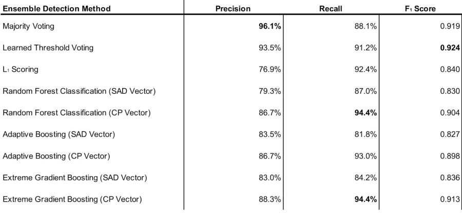
Table 2: Precision, recall, and F1 values for ensemble detection methods in detecting adversarial examples.
The results of the ensemble detection methods described in Section 3.3 are summarized in
Table 2. The voting methods performed quite well and achieved the two highest F 1scores of
all the methods discussed in this paper. This may be attributed to the high precisions and low
recalls of the individual preprocessing methods described in Table 1; the relatively strict
voting threshold of votes needed for an adversarial declaration capitalizes on the high
precision of each of the methods and is able to increase recall. The majority voting method
especially benefited from the high precisions of its constituents and yielded an extremely
voting threshold of only two votes needed for an adversarial declaration. As such, this
method was able to yield a notably higher recall than what was achieved through majority
voting, but at a noticeable cost to precision. As the Learned Threshold Voting method still
retained a fairly high precision, it achieved the overall highest F 1 score of any of the other
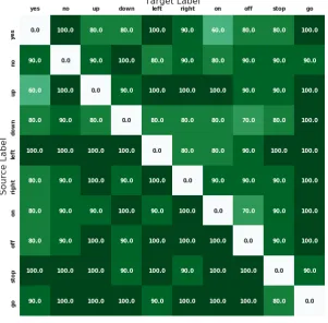
preprocessing methods. The recall values for detecting adversarial examples using the Learned Threshold Voting method are detailed in Figure 1.
The L1 Scoring method was able to achieve higher recall than either of the two voting
methods, perhaps due to its aggressive nature. However, this was achieved at the cost of
precision, which evidently lowered the F1 score.
Although tree-based classification algorithms can be quite powerful in a variety of situations,
the tree-based methods were not able to perform as well as the voting methods in detecting
adversarial examples using SAD vectors. This may be because the SAD vectors fed into the
tree algorithms discarded important voter-specific information. In particular, the vector of
summed absolute differences effectively anonymizes the voters in the ensemble; it inherently
considers each member of the ensemble equally.
This discarded information proved to be quite crucial for effectively detecting adversarial
examples, as the tree-based classification methods performed significantly better with CP
vectors (which are highly conservative). In particular, the extreme gradient boosting and
adaptive boosting classification algorithms were able to yield the highest recall values for
detecting adversarial examples out of all of the detection methods discussed in this research.
Considering that the tree-based classification methods performed significantly better with the
voter-specific information available in the CP vector, it is worth noting that the Learned
Threshold Voting method, which yielded a higher F 1 score than any tree-based classification
method, does not use voter-specific information; each vote carries equal weight towards
breaking the learned threshold. As such, it may be possible that the tree-based classification
methods outperform the Learned Threshold Voting method on larger datasets, as it could be
that this training dataset was not sufficiently large enough for learning how to optimally use
an 84-dimensional vector for classification. However, given the heavy reliance of training
data that the tree-based classification methods exhibit, they are likely not as well-suited for
flexibly handling different types of attacks as the voting methods.
As the Learned Threshold Voting method performed better over all other detection methods
discussed in this paper, it can be helpful to examine the adversarial examples that remain
undetected by this method and the benign signals that get incorrectly flagged as adversarial.
One method of analyzing the adversarial examples is by examining the average frequency
level throughout the signal. Since we are able to recover the original, clean source for each
adversarial example, we can examine the difference between the average frequencies of each
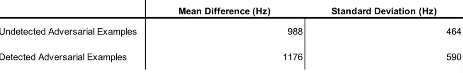
adversarial example and its clean source. The means and standard deviations of this
difference for undetected and detected adversarial examples are depicted in Table 3.
Table 3: Mean and Standard Deviation of Differences of Average Frequencies for undetected and detected adversarial examples.
found to be less than the difference in detected adversarial examples with 99% statistical
significance. This suggests that the frequencies of adversarial perturbations in the undetected
adversarial examples were concentrated at lower frequencies than those of detected
adversarial examples. As human speech is found within these lower frequencies, it is much
more difficult to disrupt or detect these adversarial examples without distorting the speech in
the signal. This may explain why these adversarial examples remained undetected under the
Learned Threshold Voting method. As a side effect, these undetected adversarial examples
with significant perturbation in the lower frequency bands would theoretically be more
perceptibly noisy to humans, as the physiology of the inner ear is fine-tuned for picking up
auditory information at these frequencies [16].
Benign examples that were falsely detected as adversarial also exhibited an interesting
property. In particular, the Speech Commands model achieved a classification accuracy of
92.7% on raw benign examples that were not detected as adversarial, but that accuracy fell to
40.4% for raw benign examples that were falsely detected as adversarial. The relatively low
classification accuracy for the benign examples flagged as adversarial suggests that even
benign examples that are classified incorrectly by the model exhibits some volatility of
outputted predictions upon preprocessing, similar to adversarial examples. For reference, the
model achieved 90.3% classification accuracy in general over all benign examples.
5. Conclusion and Future Work
Although the results of this research suggest that ensembles of audio preprocessing can be
highly effective for detecting adversarial examples, it is important to note the drawbacks of
the defenses discussed in this paper. An analysis of adversarial examples that went undetected by the Learned Voting Threshold method implied that those examples had more
adversarial perturbations in the lower frequency bands than the adversarial examples that
were detected. This suggests that attacks can optimize adversarial examples robust to the
Learned Threshold Voting method by concentrating adversarial perturbations within the
frequency range of human speech.
Although using ensemble detection methods may provide marginal security over using isolated preprocessing detection methods, recent work has shown that adaptive attacks on
squeezing ensemble of Xu, et al.; this work could be applied to attack speech recognition
models. Future work can be done in investigating stronger ensembles for detecting audio
adversarial examples and other defenses that can withstand adaptive attacks. Considering the
faceted usefulness of Speex compression for detecting adversarial examples, perhaps further
investigation into speech coding for defending against adversarial attacks is warranted.
Nevertheless, this paper demonstrated that methods of audio preprocessing can be used to
detect adversarial examples produced by the attack of Alzantot et al. on Speech Commands.
Additionally this paper examined the effectiveness of various ensembles of audio
preprocessing detection methods for defending against adversarial examples. While these
detection methods may not be extremely effective against more adaptive attacks, this research
aimed ultimately to further discussion of defenses against adversarial examples within the
audio domain: a field in desperate need of more literature.
Acknowledgments
We are thankful to the reviewers for helpful criticism, and the UCCS LINC and VAST labs
for general support. This work is supported by the National Science Foundation under Grant
No. 1659788. Any opinions, findings, and conclusions or recommendations expressed in the
material are those of the author(s) and do not necessarily represent the views of the National
Science Foundation.
References
[1] C. Szegedy, W. Zaremba, I. Sutskever, J. Bruna, D. Erhan, I. J. Goodfellow, and R. Fergus, “Intriguing properties of neural networks,” in International Conference on
Learning Representations, 2014.
[2] I. J. Goodfellow, J. Shlens, and C. Szegedy, “Explaining and harnessing adversarial examples,” in International Conference on Learning Representations, 2015.
[3] M. Alzantot, B. Balaji, and M. Srivastava, “Did you hear that? adversarial examples against automatic speech recognition,” in 31st Conference on Neural Information
Processing Systems (NIPS), 2017.
[4] N. Carlini and D. Wagner, “Audio adversarial examples: Targeted attacks on speech-to-text,” in 1st IEEE Workshop on Deep Learning and Security, 2018.
[5] A. E. Aydemir, A. Temizel, and T. T. Temizel, “The effects of JPEG and JPEG2000
2018.
[6] A. Graese, A. Rozsa, and T. E. Boult, “Assessing threat of adversarial examples on deep neural networks,” in 15th IEEE International Conference on Machine Learning and
Applications (ICMLA), 2016.
[7] A. Prakash, N. Moran, S. Garber, A. DiLillo, and J. Storer, “Deflecting adversarial attacks with pixel deflection,” in IEEE/CVF Conference on Computer Vision and Pattern
Recognition (CVPR), 2018.
[8] Z. Yang, B. Li, P.-Y. Chen, and D. Song, “Towards mitigating audio adversarial
perturbations,” 2018. [Online]. Available: https: //openreview.net/forum?id=SyZ2nKJDz
[9] D. Lemmond and R. Fitzgibbons, “Adversarial examples in audio,” 2018, CS4860 Final Project Report, University of Colorado, Colorado Springs Spring 2018.
[10] J.-M. Valin, “Speex: A free codec for free speech,” in Proceedings of linux.conf.au, 2006.
[Online]. Available: https://arxiv.org/abs/1602. 08668
[11] J.-M. Valin, K. Vos, and T. B. Terriberry, “Definition of the Opus audio codec,” RFC
6716, 2012.
[12] M. R. Schroeder and B. S. Atal, “Code-excited linear prediction (CELP): High-quality speech at very low bit rates,” in IEEE International Conference on Acoustics, Speech and
Signal Processing, 1985, pp. 937– 940.
[13] W. Xu, D. Evans, and Y. Qi, “Feature Squeezing: Detecting Adversarial Examples in Deep Neural Networks,” 2018 Network and Distributed System Security Symposium
(NDSS’18), Feb. 2018.
[14] P. Warden, “Speech commands: A dataset for limited-vocabulary speech recognition,” arXiv preprint, no. 1804.03209, 2018.
[15] T. N. Sainath and C. Parada, “Convolutional neural networks for small-footprint keyword
spotting,” in INTERSPEECH, 2015.
[16] R. L. Warren, S. Ramamoorthy, N. Ciganović, Y. Zhang, T. M. Wilson, T. Petrie, R. K.
Wang, S. L. Jacques, T. Reichenbach, A. L. Nuttall, and A. Fridberger, “Minimal basilar
membrane motion in low-frequency hearing,” Proceedings of the National Academy of Sciences, vol. 113, no. 30, Jul. 2016.
[17] W. He, J. Wei, X. Chen, N. Carlini, and D. Song, “Adversarial example defense: Ensembles of weak defenses are not strong,” in 11th USENIX Workshop on Offensive