Learning of word sense disambiguation rules by Co-training,
checking co-occurrence of features
Hiroyuki Shinnou
∗∗Ibaraki University
4-12-1 Nakanarusawa Hitachi Ibaraki 316-8511 JAPAN [email protected]
Abstract
In this paper, we propose a method to improve Co-training and apply it to word sense disambiguation problems. Co-training is an unsupervised learning method to overcome the problem that labeled training data is fairly expensive to obtain. Co-training is theoretically promising, but it requires two feature sets with the conditional independence assumption. This assumption is too rigid. In fact there is no choice but to use incomplete feature sets, and then the accuracy of learned rules reaches a limit. In this paper, we check co-occurrence between two feature sets to avoid such undesirable situation when we add unlabeled instances to training data. In experiments, we applied our method to word sense disambiguation problems for the three Japanese words ‘koe’, ‘toppu’ and ‘kabe’ and demonstrated that it improved Co-training.
1.
Introduction
In this paper, we improve Co-training by checking co-occurrence between two feature sets, and apply the pro-posed method to the word sense disambiguation problem.
Many problems in natural language processing can be converted into classification problems, and be solved by an inductive learning method. This strategy has been very suc-cessful, but it has a serious problem that an inductive learn-ing method requires labeled trainlearn-ing data, which is expen-sive because it must be made manually.
To overcome this problem, unsupervised learning meth-ods to use unlabeled training data have been proposed recently(Yarowsky, 1995)(Nigam et al., 2000)(Joachims, 1999)(Park et al., 2000). In these methods, Co-training(Blum and Mitchell, 1998) is widely cited because it is theoretically supported by the PAC learning theory.
Co-training requires two independent feature sets. First it constructs a classifier based on one feature set. The clas-sifier assigns classes to instances in an unlabeled data set, and then instances with top-ranking reliabilities of their la-bels are added to the labeled training set. These instances are added to the labeled training data. By the same proce-dure, through the other feature set some instances are added to the labeled training data. Through these procedures, Co-training augments the labeled Co-training data, and as a re-sult the accuracy of learned classifiers is improved. The mechanism in Co-training assumes that two feature sets are independent. Owing to this assumption, instances added through one feature set are regarded as random samples for another feature set. In summary, one classifier presents la-beled instances which are informative for another classifier, mutually. Co-training is efficient and practical; it has been applied to a text classification problem(Blum and Mitchell, 1998), and a named entry task(Collins and Singer, 1999).
However, it is difficult to make arrangements for two in-dependent feature sets, and in fact there is no choice but to use incomplete feature sets. Fortunately even by using in-complete feature sets, the accuracy of the classifier learned through Co-training is improved in many cases, but the ac-curacy reaches a limit. In this paper, we give an overview
of this cause, and propose a method to avoid such undesir-able situation. The principle of our method is to check co-occurrence between two feature sets. If co-co-occurrence be-tween two feature sets of the instance of interest is strong, we take the next candidate instance. The accuracy raised through Co-training is further raised by our method.
In experiments, we learned word sense disambiguation rules for three words by our method. The experiments showed that our method can improve Co-training.
2.
Co-training
The algorithm of Co-training is as follows(Blum and Mitchell, 1998).
step 0 Prepare a small amount of labeled dataLand a large amount of unlabeled dataU.
step 1 Make a setUby randomly picking upuinstances fromU.
step 2 Learn a classifierh1through a feature setx1andL. step 3 Learn a classifierh2through a feature setx2andL. step 4 Label all instances inUby usingh1,and selectp positive instances andnnegative instances in order of reliability.
step 5 Label all instances inUby usingh2,and selectp positive instances andnnegative instances in order of reliability.
step 6 Add 2p+ 2n labeled instances obtained through steps 4 and 5 toL.
step 7 Go back to step 1 and iterate the above steps.
The numbersu, p, andnused in the above algorithm depend on the targeted problem.
the feature setx2can learn a more accurateh2than the pre-cedingh2.In the same way, step 5 makesh1more accurate. In short, Co-training works well because one feature set can provide informative labeled instances to another feature set. The conditional independence assumption onx1andx2 assures that the instances selected in step 4 (and 5) are ran-dom from the view of the feature setx2(andx1.) The rea-son is given below.
In Co-training, the set of instances X is two dimen-sional. That is,Xis represented by(X1, X2).LetDbe the distribution onX,and letf,f1 andf2be target functions onX,X1 andX2 respectively. The conditional indepen-dence assumption onx1andx2is defined by the following two equations.
P r[x2= ˆx2|x1= ˆx1] =P r[x2= ˆx2|f1(x1) =f1(ˆx1)] (1) P r[x1= ˆx1|x2= ˆx2] =P r[x1= ˆx1|f2(x2) =f2(ˆx2)] (2)
Because steps 4 and 5 are symmetric regardingx1and x2,we concentrate only on step 4 in the remaining
expla-nation.
Let(ˆx1,xˆ2)be a positive instance selected through step 4.
The left part of (1) represents the probability that the instance randomly picked up from the following set Ais equal to(ˆx1,ˆx2).
A={(x1, x2)∈D|x1= ˆx1}
In other words, this probability implies the empirical prob-ability that(ˆx1,xˆ2)is selected from the judgement of the feature setxˆ1. On the other hand, the right part of (1) repre-sents the probability that the instance randomly picked up from the positive instances inDis equal to(x1,ˆx2). There-fore, for the feature setx2, the instance(ˆx1,xˆ2)is regarded as a random sample from the positive instances in D.In the same way, the instances which are regarded as random samples from the negative instances inDare also picked up through step 4. The number of instances picked from the positive instances and the number of instances picked from the negative instances, that is pandn, are fixed through the ratio of the number of positive instances and the num-ber of negative instances inD. Therefore, the addedp+n instances are regarded as random samples picked up from D.
3.
Checking co-occurrence between feature
sets
Actually, it is difficult to make arrangements for two in-dependent feature sets. In practical natural language prob-lems, many features are generally relevant to other features, so the required assumption in Co-training is violated. If the co-occurrence between xˆ1 and ˆx2 is strong, the value of the following equation is higher than the probability that another instance(x2,xˆ1)is picked up.
P r[x2= ˆx2|x1= ˆx1]
Therefore it is clear that (1) is violated. In a practical pro-cess, if the instance(ˆx1,xˆ2)is added toLthrough step 4,
the nexth2 learned through thatLjudgesxˆ2confidently. In this case,(ˆx1,xˆ2)is added toL again because the co-occurrence betweenˆx1 andxˆ2is strong. If this process is iterated, neitherx1norx2can gain informative instances. As a result, the accuracy of the learned classifier reaches its limit.
To avoid such undesirable situation, we take the strat-egy that we do not add the instance (ˆx1,ˆx2)but the next candidate instance toL, if the co-occurrence betweenxˆ1 andˆx2is strong.
We should note that the co-occurrence betweenˆx1and
ˆ
x2 must be computed not on all of data setD but on the
labeled dataL.Moreover, the occurrence is not the co-occurrence between instances but the co-co-occurrence be-tween feature sets. We can define our co-occurrence by extending a measure of the co-occurrence between features.
4.
Application to word sense disambiguation
In this paper, we apply our method to word sense disam-biguation problems. A word sense disamdisam-biguation problem can be regarded as the problem of judging which meaning of a wordwthat appeared in contextbis positive or neg-ative1. This problem is just a classification problem. Thekey is what features we should use to solve the problem. 4.1. Setting of feature sets
Co-training requires two feature sets that are as inde-pendent as possible. For this requirement, we divide the context on the word winto two types of context, that is, the left contextbland the right contextbr.The left context is actually a line of words to the left of w,and the right context is a line of words to the right ofw.The feature set derived fromblisx1,and the feature set derived frombris x2.
Let’s consider an example. The Japanese word ‘koe’ is ambiguous because it has two meanings: one is “opinion” and another is “sound2.” The meaning of ‘koe’ in the
fol-lowing sentence is “opinion.”
nihon kokumin no koe wo atume masita
In the above sentence,blof ‘koe’ is “nihon kokumin no” andbrof ‘koe’ is “wo atume masita.”
Frombl,we extract three types of features:l1,l2, and
l3. In the same way, we extract three types of features frombr:r1,r2, andr3. Table 1 shows the definitions of these features.
In the case that we focus on the word ’koe’ in the above example sentence, the following six features are extracted.
l1 = no
l2 = kokumin-no
l3 = nihon-kokumin-no r1 = wo
r2 = wo-atumeru r3 = wo-atumeru-masu
1
In this paper, we assume that the number of meanings of the word is two if the word is ambiguous.
2
Feature name Feature value
l1 (the 1st word from the left)
l2 (the 2nd word)-(the 1st word from the left)
l3 (the 3rd word)-(the 2nd word)-(the 1st word from the left)
r1 (the 1st word to the right)
r2 (the 1st word)-(the 2nd word to the right)
r3 (the 1st word)-(the 2nd word)-(the 3rd word to the right)
Table 1: Arranged features
Our defining two feature sets,x1andx2, have a certain degree of independence.
Co-training requires a single learning method to learn a classifier through each feature set. In this pa-per, as the learning method we take the decision list method(Yarowsky, 1994).
4.2. Measurement of co-occurrence
We define the strength of co-occurrence between two feature sets,xˆ1andxˆ2,Cor(ˆx1,ˆx2)as the following equa-tion.
Cor(ˆx1,ˆx2) = maxi,j dice(ˆli,rjˆ)
In this equation,dice(ˆli,rjˆ)is the dice coefficient be-tweenliˆandrj,ˆ defined as the following equation.
dice(ˆli,rjˆ) = 2frq(ˆli,rjˆ) frq(ˆli) +frq( ˆrj)
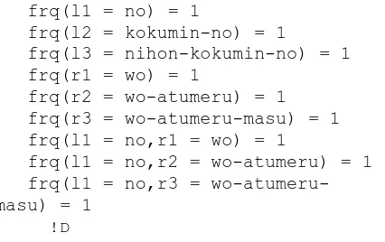
In this equation,frq(X)represents the frequency of the featureXinL,andfrq(X, Y)represents the frequency of instances which have both the featureXand the featureY. For example, we assume thatLconsists of one instance that has the following six features.
l1 = no
l2 = kokumin-no
l3 = nihon-kokumin-no r1 = wo
r2 = wo-atumeru r3 = wo-atumeru-masu
In this case, we obtain the following frequencies. With these frequencies, we can calculate co-occurrence between two feature sets.
frq(l1 = no) = 1
frq(l2 = kokumin-no) = 1
frq(l3 = nihon-kokumin-no) = 1 frq(r1 = wo) = 1
frq(r2 = wo-atumeru) = 1 frq(r3 = wo-atumeru-masu) = 1 frq(l1 = no,r1 = wo) = 1
frq(l1 = no,r2 = wo-atumeru) = 1 frq(l1 = no,r3 = wo-atumeru-masu) = 1
!D
frq((l3 = nihon-kokumin-no,r3 = wo-atumeru-masu) = 1
5.
Experiments
We apply our method to learning of a classifier to judge the meaning of the word ’koe’. The Japanese word ’koe’ usually means “opinion” or “sound.” In this experiment, to exclude vague judgment, we assume that ’koe’ has just two meanings, that is “opinion” and “not opinion.” We take the former as positive and the latter as negative.
Next, we extracted sentences including the word ’koe’ from five years’ worth of Mainichi newspaper articles (from ’93 to ’97). In all, we got 30,458 sentences. Next, we randomly picked up 100 sentences and 500 sentences from these sentences, and assigned a positive label or a negative label to each sentence according to the meaning of ’koe’ in the sentence. The labeled 100 sentences are the labeled training dataL,and the labeled 500 sentences are the test dataT.The remaining 29,858 sentences are the unlabeled training dataU.The parameteru, which is the number of instances picked up fromU in each Co-training iteration, was set at 50, and both of the parameterspandn, which are the number of positive and negative instances added to Lin each Co-training iteration respectively, were set at 3.
In order to measure the strength of co-occurrence of fea-ture sets, strictly speaking, we must count the frequencies of features in every Co-training iteration becauseLchanges in every iteration. However, for efficiency, we conduct such counting once every 50 iterations.
The added instances are basically selected in order of reliability of the label assigned by the classifier learned throughL. Because we use the decision list as the classifier, we can use the order of the decision list as the reliability of the label. Even if the reliability of the label assigned to the instance (ˆx1,ˆx2),is very high, the instance is not se-lected and the next candidate is sese-lected if the strength of co-occurrence between xˆ1andxˆ2, that isCor(ˆx1,ˆx2), is greater than 0.3. The value 0.3 was fixed empirically.
Figure 1 shows the result of our experiment. In the figure, the x-axis shows the repetition of Co-training and the y-axis shows the precision for the test data T. The graph ’original’ shows the learning of original Co-training, and the curved line ’our method’ shows the learning of our method. As this figure shows, Co-training boosts the per-formance of the general classifier learned through only ini-tial labeled data. However, the original Co-training reaches a limit, about 0.77. On the other hand, our method further boosts the performance of the classifier improved by the original Co-training.
We experimented with the word ’toppu’ and the word
0.64 0.66 0.68 0.7 0.72 0.74 0.76 0.78 0.8 0.82 0.84
0 100 200 300 400 500 600
’our_method’ ’original’
Figure 1: Co-training and our method (’koe’)
’toppu’ usually means “top” or “chief executive.” We take
the meaning “top” as positive and other meanings as neg-ative. The Japanese word ’kabe’ usually means “wall” or “obstacle.” We take the meaning “wall” as positive and other meanings as negative. Table 2 shows parameters used in the experiments.
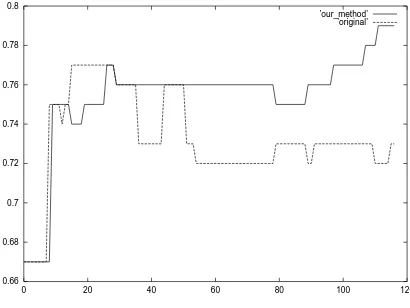
Figures 2 and 3 show the result of ’toppu’ and ’kabe’ respectively. The same as the result of ’koe’, both figures show that our method improves Co-training.
0.73 0.74 0.75 0.76 0.77 0.78 0.79 0.8
0 50 100 150 200 250 300
’our_method’ ’original’
Figure 2: Co-training and our method (’toppu’)
0.66 0.68 0.7 0.72 0.74 0.76 0.78 0.8
0 20 40 60 80 100 120
’our_method’ ’original’
Figure 3: Co-training and our method (’kabe’)
Table 3 shows the maximum value achieved in each ex-periment. The baseline is the precision of the general clas-sifier learned through only initial labeled data.
|L| |U| |T| u p n
’koe’ 100 29,858 500 50 3 3
’toppu’ 100 14,569 300 50 3 1
’kabe’ 100 5,866 100 50 3 2
Table 2: Parameter used in experiments
Baseline Original Our method Co-training
’koe’ 0.636 0.774 0.824
’toppu’ 0.743 0.787 0.793
’kabe’ 0.670 0.770 0.790
Table 3: Maximum precision
6.
Discussions
The applicability of Co-training for a classification problem depends on the independence of two feature sets. Independence of two feature sets actually corresponds to in-dependent view points which are clues to judge the classes. In the web page classification problem, words occurring on the page and words occurring in hyperlinks that point to that page can be regarded as two independent clues to judge the classes(Blum and Mitchell, 1998). In the named entity task, which can generally be solved by converting to a classification problem, words occurring in the named entity expression and context surrounding that expression can be regarded as two independent clues to judge the classes(Collins and Singer, 1999). In this paper, for the word sense disambiguation problem we proposed the left context and the right context as two independent clues. These clues are inspired by the idea that we can judge the meaning of a noun word only by words modifying that noun, and can also judge the meaning of that noun by the verb word which has that noun in a case slot. For example, the meaning of the word ’koe’ in the phrase ’nihon
koku-min no koe’ can be judged as “opinion” easily. Moreover
the meaning of the word ’koe’ in the phrase ’koe wo atume
masita’ can also be judged as “opinion” easily. Based on
our idea, our method can only handle nouns. Moreover, the effective feature for a word sense disambiguation de-pends on the target word. Therefore, the words our method can handle may be limited. It is important to set up many features and then to divide them into two independent sets automatically.
of labeled instances approximate the distribution of all in-stances. However, we cannot add an instance to labeled training data unless that instance has a reliable label. In Co-training, because of the conditional independence as-sumption, we only have to add an instance with a reliable label to labeled training data to adjust the distribution la-beled instances automatically. If the conditional indepen-dence assumption is broken, the adjustment of the distribu-tion labeled instances is also broken. Our method adopts a strategy to avoid such broken adjustment. Of course, the risk of our method adding an instance with a wrong label to labeled training data is bigger than the risk of Co-training doing so, because our method may select an instance with a less reliable label through the condition of co-occurrence. If an instance with a wrong label is added to labeled train-ing data, the precision of the learntrain-ing classifier drops grad-ually. In short, our method avoids the broken adjustment at the risk of adding an instance with a wrong label to la-beled training data. In our experiments, the threshold of the co-occurrence strength to reject the instance is fixed at 0.3. Because we can know the distribution of all instances, we can take other thresholds according to the instance of interest. This investigation will be left for future work.
Besides Co-training, there are other methods to boost the performance of a classifier by using unlabeled data. The method to combine the EM algorithm and naive Bayes(Nigam et al., 2000) and the Transductive method(Joachims, 1999) have been proposed. Both meth-ods handle text classification problems. These methmeth-ods have the advantage that they do not require independent fea-ture sets. However, the EM algorithm method assumes that the data are produced by a mixture model, and there is one-to-one correspondence between mixture components and classes. It is unknown whether the assumed model is ap-posite to a word sense disambiguation problem. Moreover there is a report that Co-training was superior to the EM algorithm method in some experiments(Nigam and Ghani, 2000). Meanwhile the Transductive method requires too much computational cost, and so is not practical for prob-lems with a large amount of unlabeled data. Thus, Co-training is efficient and practical only if two independent feature sets can be found for the target problem. There-fore it is important to relax that condition, like our method. On the other hand, more than one classifier in the Bag-ging method(Breiman, 1996) may be substituted for inde-pendent feature sets. The method to add instances to la-beled data by Bagging has been proposed(Park et al., 2000). Furthermore, we estimate that Co-training highly relevant to Boosting(Freund and (translation by Naoki Abe), 1999) and an active learning method called “Query by Commit-tee”(Seung et al., 1992). In the future we will investigate the relationships among these learning methods.
7.
Conclusions
Co-training is an efficient and practical method to boost the performance of a classifier by using a small amount of labeled data and a large amount of unlabeled data. How-ever, Co-training requires two feature sets with the condi-tional independence assumption. Because this assumption is too rigid, the accuracy of learned rules reaches a limit.
In this paper, we investigated the cause of this, and pro-posed a method to avoid such undesirable situation. In our method, if the co-occurrence between feature sets of the current candidate instance is strong, we select the next can-didate instance.
In experiments, we applied our method to word sense disambiguation problems for the three words ‘koe’, ‘toppu’ and ‘kabe’ and demonstrated that it improved Co-training.
In the future, we will try to take other thresholds ac-cording to the instance of interest, and clarify the relation-ships among Co-training, Boosting and an active learning method.
8.
References
Avrim Blum and Tom Mitchell. 1998. Combining Labeled and Unlabeled Data with Co-Training. In 11th Annual
Conference on Computational Learning Theory (COLT-98), pages 92–100.
Leo Breiman. 1996. Bagging predictors. Machine
Learn-ing, 24(2):123–140.
Michael Collins and Yoram Singer. 1999. Unsupervised Models for Named Entity Classification. In 1999 Joint
SIGDAT Conference on Empirical Methods in Natural Language Processing and Very Large Corpora, pages
100–110.
Yoav Freund and Robert Schapire (translation by Naoki Abe). 1999. A short introduction to boost-ing (in japanese). Journal of Japanese Society for Artificial Intelligence, 14(5):771–780.
Thorsten Joachims. 1999. Transductive inference for text classfication using support vector machines. In 16th
In-ternational Confernece on Machine Leaning (ICML-99),
pages 200–209.
Kamal Nigam and Rayid Ghani. 2000. Analyzing the ef-fectiveness and applicability of co-trainig. In 9th
In-ternational Conference on Information and Knowledge Management, pages 86–93.
Kamal Nigam, Andrew McCallum, Sebastian Thrun, and Tom Mitchell. 2000. Text classification from labeled and unlabeled documents using em. In Machine
Learn-ing, volume 39, pages 103–134.
Seong-Bae Park, Byoung-Tak Zhang, and Yung Taek Kim. 2000. Word sense disambiguation by learning from un-labeled data. In 38th Annual Meeting of the Association
for Computational Linguistics (ACL-00), pages 547–
554.
H. S. Seung, M. Opper, and H. Sompolinsky. 1992. Query by committee. In 5th annual workshop on
Computa-tional Learning Theory (COLT-92), pages 287–294.
David Yarowsky. 1994. Decision lists for lexical ambiguity resolution: Application to accent restoration in spanish and french. In 32th Annual Meeting of the Association
for Computational Linguistics (ACL-94), pages 88–95.
David Yarowsky. 1995. Unsupervised word sense disam-biguation rivaling supervised methods. In 33th Annual