Signal Processing Algorithms for MIMO Radar

Thesis by

Chun-Yang Chen

In Partial Fulfillment of the Requirements for the Degree of

Doctor of Philosophy

California Institute of Technology Pasadena, California

2009

c

2009

Acknowledgments

First of all, I would like to thank my advisor, Professor P. P. Vaidyanathan, for his excellent guidance and support during my stay in Caltech. He has taught me everything I need to be a great researcher including being creative, thinking deeply, and the skills for presenting ideas and writing papers. He is also a perfect gentleman who is always nice, polite, and considerate. He is a perfect role model and I have learned so much from him.

I also like to thank the members of my defense and candidacy committees: Professor Abu-Mostafa, Professor Babak Hassibi, Professor Ho, Dr. Tkacenko , and Dr. van Zyl. I would also like to thank the National Science Foundation (NSF), and the Office of Naval Research (ONR) for their generous financial support during my graduate studies at Caltech.

I also like to thank my labmates Professor Byung-Jun Yoon, Dr. Borching Su, Ching-Chih Weng, Piya Pal, and Chih-Hao Liu. It was truly a great experience working with these smart people. I will deeply miss our discussions and conversations as well as the many conference trips that we made together. I also would like to thank Andrea Boyle, our wonderful secretary, for her kind assistance and professional support.

Also, I would like to thank my parents, Tien-Mu Chen and Shu-Fen Yang, for their love and support for my entire life. I also want to thank my brother Chun-Goo Chen for taking care of my parents for me in Taiwan. I would like to give a special thanks to my lovely wife Chia-Wen Chang for her accompany and love.

Abstract

Radar is a system that uses electromagnetic waves to detect, locate and measure the speed of re-flecting objects such as aircraft, ships, spacecraft, vehicles, people, weather formations, and terrain. It transmits the electromagnetic waves into space and receives the echo signal reflected from ob-jects. By applying signal processing algorithms on the reflected waveform, the reflecting objects can be detected. Furthermore, the location and the speed of the objects can also be estimated. Radar was originally an acronym for “RAdio Detection And Ranging”. Today radar has become a stan-dard English noun. Early radar development was mostly driven by military and military is still the dominant user and developer of radar technology. Military applications include surveillance, nav-igation, and weapon guidance. However, radar now has a broader range of applications including meteorological detection of precipitation, measuring ocean surface waves, air traffic control, police detection of speeding traffic, sports radar speed guns, and preventing car or ship collisions.

systems in many different aspects. However, it also generates some issues. It increases the number of dimensions of the received signals. Consequently, this increases the complexity of the receiver. Furthermore, the MIMO radar transmits an incoherent waveform on each of the transmitting anten-nas. This in general reduces the processing gain compared to the phased array radar. The multiple arbitrary waveforms also affects the range and Doppler resolution of the radar system.

The second half of the thesis focuses on the transmitted waveform design for MIMO radar sys-tems. We first study the ambiguity function of the MIMO radar and the corresponding waveform design methods. In traditional (SIMO) radars, the ambiguity function of the transmitted pulse char-acterizes the compromise between range and Doppler resolutions. It is a major tool for studying and analyzing radar signals. The idea of ambiguity function has recently been extended to the case of MIMO radar. In this thesis, we derive several mathematical properties of the MIMO radar ambi-guity function. These properties provide some insights into the MIMO radar waveform design. We also propose a new algorithm for designing the orthogonal frequency-hopping waveforms. This algorithm reduces the sidelobes in the corresponding MIMO radar ambiguity function and makes the energy of the ambiguity function spread evenly in the range and angular dimensions. Therefore the resolution of the MIMO radar system can be improved. In addition to designing the waveform for increasing the system resolution, we also consider the joint optimization of waveforms and re-ceiving filters in the MIMO radar for the case of extended target in clutter. An extended target can be viewed as a collection of infinite number of point targets. The reflected waveform from a point target is just a delayed and scaled version of the transmitted waveform. However, the reflected waveform from an extended target is a convolved version of the transmitted waveform with a tar-get spreading function. A novel iterative algorithm is proposed to optimize the waveforms and receiving filters such that the detection performance can be maximized. The corresponding itera-tive algorithms are also developed for the case where only the statistics or the uncertainty set of the target impulse response is available. These algorithms guarantee that the SINR performance improves in each iteration step. The numerical results show that the proposed iterative algorithms converge faster and also have significant better SINR performances than previously reported algo-rithms.1

Contents

Acknowledgments iii

Abstract iv

1 Introduction 1

1.1 Basic Review of Radar . . . 1

1.1.1 Detection and Ranging . . . 1

1.1.2 Estimation of the Velocity . . . 5

1.1.3 Beamforming . . . 8

1.2 Review of MIMO Radar . . . 11

1.2.1 The Virtual Array Concept . . . 12

1.3 Outline of the Thesis . . . 17

1.3.1 Robust Beamforming — Chapter 2 . . . 18

1.3.2 Efficient Space-Time Adaptive Processing — Chapter 3 . . . 19

1.3.3 Ambiguity Function and Waveform Design — Chapter 4 . . . 19

1.3.4 Joint Transmitted Waveform and Receiver Design — Chapter 5 . . . 20

1.4 Notations . . . 20

2 Robust Beamforming 22 2.1 Introduction . . . 22

2.2 MVDR Beamformer and the Steering Vector Mismatch . . . 24

2.3 Previous Work On Robust Beamforming . . . 26

2.3.1 Diagonal Loading Method . . . 26

2.3.2 LCMV Method . . . 27

2.3.4 General-Rank Method . . . 28

2.4 New Robust Beamformer . . . 28

2.4.1 Frequency Domain View of the Problem . . . 29

2.4.2 Two-Point Quadratic Constraint . . . 30

2.4.3 Two-Point Quadratic Constraint with Diagonal Loading . . . 34

2.5 Numerical Examples . . . 37

2.6 Conclusions . . . 50

3 Space-Time Adpative Processing for MIMO Radar 51 3.1 Introduction . . . 51

3.2 STAP in MIMO Radar . . . 53

3.2.1 Signal Model . . . 53

3.2.2 Fully Adaptive MIMO-STAP . . . 56

3.2.3 Comparison with SIMO System . . . 58

3.2.4 Virtual Array . . . 59

3.3 Clutter Subspace in MIMO Radar . . . 60

3.3.1 Clutter Rank in MIMO Radar . . . 61

3.3.2 Data Independent Estimation of the Clutter Subspace with PSWF . . . 64

3.4 New STAP Method for MIMO Radar . . . 67

3.4.1 The Proposed Method . . . 67

3.4.2 Complexity of the New Method . . . 68

3.4.3 Estimation of the Covariance Matrices . . . 69

3.4.4 Zero-Forcing Method . . . 69

3.4.5 Comparison with Other Methods . . . 70

3.5 Numerical Examples . . . 71

3.6 Conclusions . . . 75

4 Ambiguity Function of the MIMO Radar and the Waveform Optimization 76 4.1 Introduction . . . 76

4.2 Review of MIMO Radar Ambiguity Function . . . 78

4.3 Properties of The MIMO Radar Ambiguity Function for ULA . . . 81

4.5 Frequency-Hopping Pulses . . . 90

4.6 Optimization of the Frequency-Hopping Codes . . . 92

4.7 Design Examples . . . 94

4.8 Conclusions . . . 97

5 Waveform Optimization of the MIMO Radar for Extended Target and Clutter 100 5.1 Introduction . . . 100

5.2 Problem Formulation and Review . . . 103

5.2.1 Problem Formulation . . . 105

5.2.2 Review of Pillai’s method [82] . . . 107

5.3 Proposed Iterative Method . . . 108

5.4 Iterative Method with Random and Uncertain Target Impulse Response . . . 112

5.4.1 Random Target Impulse Response . . . 112

5.4.2 Uncertain Target Impulse Response . . . 115

5.5 Numerical Examples . . . 121

5.6 Conclusions . . . 127

5.7 Appendix . . . 127

6 Conclusion 130 6.1 Future Work . . . 131

List of Figures

1.1 Basic radar for detection and ranging . . . 2

1.2 Matched filter in the radar receiver . . . 3

1.3 The LFM signal: (a) real part of an LFM waveform and (b) Fourier transfrom magni-tude of the LFM waveform . . . 4

1.4 Illustration of the Doppler effect . . . 6

1.5 The pulse train . . . 6

1.6 Doppler processing . . . 8

1.7 Ranger, azimuth angleθ, and elevation angleφ . . . 9

1.8 A uniform linear antenna array (ULA) . . . 10

1.9 (a) A MIMO radar system withM = 3andN = 4. (b) The corresponding virtual array 13 1.10 (a) A ULA MIMO radar system withM = 3andN= 4. (b) The corresponding virtual array . . . 16

1.11 (a) A MIMO radar system withM = 3,N = 4anddT =dR. (b) The corresponding virtual array . . . 17

2.1 Frequency domain view of the optimization problem . . . 30

2.2 Example of a solution of the two-point quadratic constraint problem that does not satisfy|s†w| ≥1forθ1≤θ≤θ2 . . . 34

2.3 The locations of zeros of the beamformer in Fig. 2.2 . . . 34

2.4 An illustration of Algorithm 2, whereA = {w|s†(θ)w| ≥ 1, θ = θ1, θ2}and B = {w|s†(θ)w| ≥1, θ1≤θ≤θ2} . . . 37

2.5 Example 1: SINR versusγfor SNR = 10dB. . . 39

2.6 Example 1 continued: SINR versusγfor SNR = 20dB . . . 39

2.7 Example 2: SINR versus SNR . . . 41

2.9 Example 3 continued: SINR versus mismatch angle for SNR = 10dB . . . 43

2.10 Example 4: SINR versus number of antennas for SNR = 0dB . . . 44

2.11 Example 4 continued: SINR versus number of antennas for SNR = 10dB . . . 45

2.12 Example 5: SINR versus number of snapshots for SNR = 10dB . . . 47

2.13 Estimated SOI power versus number of snapshots for SNR = 10dB . . . 48

2.14 Example 6: SINR versus SNR for general type mismatch . . . 49

3.1 This figure illustrates a MIMO radar system with M transmitting antennas andN receiving antennas. The radar station is moving with speedv . . . 54

3.2 The SINR at looking direction zero as a function of the Doppler frequencies for differ-ent SIMO and MIMO systems . . . 60

3.3 Example of the signalc(x;fs,i). (a) Real part. (b) Magnitude response of Fourier trans-form . . . 63

3.4 Plot of the clutter power distributed in each of the orthogonal basis elements . . . 66

3.5 The SINR performance of different STAP methods at looking direction zero as a func-tion of the Doppler frequency . . . 72

3.6 Spatial beampatterns for four STAP methods . . . 73

3.7 Space-time beampatterns for four methods: (a) The proposed zero-forcing method, (b) Principal component (PC) method [44], (c) Separate jammer and clutter cancellation method (SJCC) [56] and (d) Sample matrix inversion (SMI) method [44] . . . 74

4.1 Examples of ambiguity functions: (a) Rectangular pulse, and (b) Linear frequency modulation (LFM) pulse with time-bandwidth product 10, whereTis the pulse duration 79 4.2 MIMO radar scheme: (a) Transmitter, and (b) Receiver . . . 79

4.3 Illustration of the LFM shearing . . . 87

4.4 Illustration of the pulse waveform . . . 88

4.5 (a) Real parts and (b) spectrograms of the waveforms obtained by the proposed method 95 4.6 (a) Real parts and (b) spectrograms of the orthogonal LFM waveforms . . . 96

4.7 Empirical cumulative distribution function of|Ω(τ, f, f0_{)|. . . . 96}

4.8 Cross-correlation functions r_m,mφ 0(τ) of the waveforms generated by the proposed method . . . 97

5.1 Illustration of (a) the signal model, and (b) the discrete baseband equivalent model . . 103 5.2 The FIR equivalent model . . . 106 5.3 Example 5.1: The parameters used in the matrix AR model (a) matrixAand (b) matrix

B . . . 122 5.4 Example 5.1: Comparison of the SINR versus number of iterations . . . 122 5.5 Example 5.1: (a)–(d) real part of the initial transmitted waveforms, (e)–(h) real part of

the transmitted four waveformsfobtained by Algorithm 1, (i)–(l) real part of the four receiving filtershobtained by Algorithm 1 . . . 123 5.6 Example 5.2: Comparison of the SINR versus CNR . . . 124 5.7 Example 5.3: Comparison of the SINR versus CNR with random target impulse response125 5.8 Example 5.4: Comparison of the worst SINR versus CNR with uncertain target

List of Tables

Chapter 1

Introduction

In this chapter, we review basic concepts from radar and MIMO radar and briefly describe the major results of each chapter. The chapter is organized as follows: Section 1.1 gives the basic review of the radar system. Section 1.2 reviews the basic concept of MIMO radar. Section 1.3 gives an outline of this thesis. Section 1.4 defines the notations used in this thesis.

1.1

Basic Review of Radar

The radar systems can be categorized intomonostaticandbistatic. The transmitter and the receiver of a monostatic radar are located in the same location while the transmitter and receiver of the bistatic radar are far apart relative to the wavelength used in the radar. According to the characteristics of the transmitted signals, the radar systems can be further categorized intocontinuous waveform radar andpulse radar. The continuous waveform radar transmits a single continuous waveform while the pulse radar transmits multiple short pulses. Most of the modern radars are monostatic pulse radars [87]. In this thesis, we will consider both continuous waveform and pulse radar. However, we will study only monostatic radar throughout this thesis.

1.1.1

Detection and Ranging

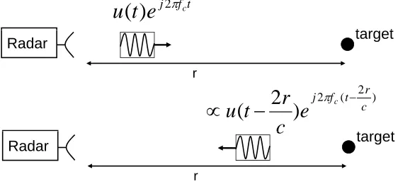
Consider a monostatic radar system with one antenna as shown in Fig. 1.1. The radar emits a waveformu(t)into the space. The waveform hits the target located in rangerand comes back to the antenna. After demodulation, the received signal can be expressed as [87]

αu(t−2r

c ) +v(t),

wherecis the speed of wave propagation,ris the range of the target,v(t)is the additive noise, and

αdenotes the amplitude response of the target. The amplitude responseαis determined by the radar cross section (RCS) of the target, the rangerof the target, the beampattern of the antenna, and the angle of the target. In the receiver, a matched filter is usually applied to enhance the

signal-t t t f j _c

e

t

u

(

)

Radar target r t t ) 2 ( 2

)

2

(

e

c

r

t

u





Radar target

r

c

Figure 1.1: Basic radar for detection and ranging

to-noise ratio (SINR). The matched filter output can be expressed as

y(τ) = Z ∞

−∞

αu(t−2r

c )u

∗_(t−τ)dt+Z ∞

−∞

v(t)u∗(t−τ)dt

= αruu(τ−

2r c ) +

Z ∞

−∞

v(t)u∗(t−τ)dt,

whereruu(τ) =

R∞

−∞u(t)u

∗_{(t−τ)dτ is the autocorrelation function ofu(t). The input-output}

re-lation is illustrated in Fig. 1.2. To determine whether there is a target, the matched filter output signal is checked at a specific time instantτ0. Ifruu(τ)> η for a predetermined thresholdη, then

∫

r

2

)

2

(

c

r

t

u

−

∫

−

−

u

t

dt

c

r

t

u

(

2

)

(

τ

)

∫

∞ −

−

⋅

u

(

t

τ

)

dt

c

matched filter

range resolution

Figure 1.2: Matched filter in the radar receiver

range of the target. For a simple point target, the range of the target can be obtained by

r= 1 2τ0c,

whereτ0is the time instant at which the matched filter output exceeds the threshold. For the case of multiple targets, the matched filter output signal can be expressed as

y(τ) =

Nt−1

X

i=0

αiruu(τ−

2ri

c ) + Z ∞

−∞

v(t)u∗(t−τ)dt,

whereNtis the number of targets,riis the range of theith target, andαiis the amplitude response

of theith target. To be able to distinguish these targets, the autocorrelation functionruu(τ)has to

be a narrow pulse in order to reduce the interferences coming from other targets. A narrow pulse in time-domain has a widely spread energy in its Fourer transform and vice versa. Therefore to obtain a narrow pulseruu(τ), one can choose the waveformu(t)so that the energy of the Fourier

transform ofruu(τ)is widely spread. Fourier transform of the autocorrelation functionruu(τ)is

expressed as

Suu(jω) =|U(jω)|2,

whereU(jω)is the Fourier transform of the waveformu(t). Therefore, one can chooseu(t)so that its energy is widely spread over different frequency components.

modulus property is the linear frequency modulated (LFM) waveform. It is also called the chirp waveform. The LFM waveform can be expressed as

u(t)∝

 



ej2πfct_ejπkt2_{, 0≤t < T}

0, otherwise.

wherefc is the carrier frequency,kis the parameter that determines the bandwidth of the signal,

and T is the duration of the signal. The instantaneous frequency of the LFM waveform is the derivative of the phase function

1 2π

d(2πfct+πkt2)

dt =fc+kt.

So the approximate bandwidth of the LFM signal iskT. The autocorrelation function of the LFM waveform can be approximated as [62]

ruu(τ)≈

  

 

sin(πkT τ(1−|τ|

T )

πkT τ

, −T ≤τ < T.

0, otherwise

Fig. 1.3 shows the LFM waveform and the corresponding autocorrelation. The first zero-crossing

0 0.1 0.2 0.3 0.4 0.5 0.6 0.7 0.8 0.9 1 −1

−0.5 0 0.5 1

real part of the LFM

−1 −0.8 −0.6 −0.4 −0.2 0 0.2 0.4 0.6 0.8 1 0

0.2 0.4 0.6 0.8 1

Time

|autocorrelation|

Figure 1.3: The LFM signal: (a) real part of an LFM waveform and (b) Fourier transfrom magnitude of the LFM waveform

been “compressed” after the matched filtering from the original widthT to 1

kT. This effect is called pulse compression. The ratio between the original width and the compressed width is defined as the compression ratio. It can be expressed as

T 1

kT =kT

2_.

We have previously mentioned that the bandwidth of the LFM signal iskT. SokT2_{= (kT)·Tis the} time-bandwidth product of the LFM signal. Thus the resolution of a radar system emitting LFM waveform is determined by the time-bandwidth product of the LFM waveform.

Another great benefit of the LFM signal is that it can be easily generated by circuits [92]. These advantages makes LFM signal the most widely used radar signal today [62, 87]. In fact, LFM signal can even be found in some natural “radar system” such as the ultrasonic systems of bats and dol-phins. We will talk more about the waveform design and introduce a useful tool called ambiguity function to analyze the waveforms in Chapter 4.

1.1.2

Estimation of the Velocity

Besides detection and ranging, radar system can be used to further measuring the velocity of an ob-ject. For example, police speed radar measures the velocity of moving vehicles. The radar systems can also use the velocity information to filter out the unwanted reflected signals. For example, for a radar system built to detect flying objects such as aircrafts or missiles, clouds will be the unwanted reflected signals. In radar community, this kind of unwanted signal is calledclutter. In most of the case, the clutter can be very strong. Sometimes it may go up to30to40dB above the target signal. Fortunately, since the clutter objects are usually still or moving slowly, one can use the velocity information to filter it out. We will explain how radar systems obtain the velocity information.

Consider a monostatic radar system with one antenna and a moving target as shown in Fig. 1.4. The target moves with the speedvat an angleθas shown in the figure. The radar system emits a narrowband waveformu(t)ej2πfct_{. Here narrowband means the bandwidth of the signal is much} smaller than the carrier frequencyfc. The waveform hits the moving target at rangerand comes

back to the antenna. After demodulation, the received waveform can be expressed as

αu(t−2r

c )e

t

t

e

t

u

(

)

v

Radar

target



cos

v



)

2

(

j c D

e

r

t

u





v

Radar

c

target



cos

v



Figure 1.4: Illustration of the Doppler effect

wherefDis the Doppler frequency,αis the amplitude response of the target andv(t)denotes the

noise in the receiver. The Doppler frequency can be expressed as [62]

fD=

c+vcosθ c−vcosθfc≈

2vcosθ c fc.

Note thatfDis much smaller than the carrier frequencyfcbecause the velocity of the objectvis

usually much smaller than the speed of light. Therefore, to effectively estimate the small Doppler frequencyfD, we will need a longer time window. One way to achieve this is to transmit multiple

pulses. These pulses can occupy a longer time window as shown in Fig. 1.5. Therefore they provide better Doppler frequency resolution. Also, the computational complexity for processing pulses is

}

Re{

e

∑

∑

−

=

lT

t

t

u

(

)

φ

(

)

Figure 1.5: The pulse train

in pulse radar can be expressed as

u(t) =

L−1

X

l=0

φ(t−lT), (1.2)

whereφ(t)is the basic shape pulse,lis the pulse index,Tis the pulse repetition period, andLis the number of the total transmitted pulses. In radar community,lis often calledslow timeindex and

tis calledfast time. The slow time is used to process the Doppler information while the fast time is used to process the range information. Fig. 1.5 illustrates a pulse train signal and the Doppler envelope. Using (1.2) and (1.1), the corresponding received signal becomes

α

L−1

X

l=0

φ(t−lT −2r

c )e

j2πfDt_+v(t).

Because the pulseφ(t)is narrow in time domain, one can approximate the Doppler termej2πfDt_as a constant within the pulse. Thus the above equation can be approximated as

α

L−1

X

l=0

φ(t−lT −2r

c )e

j2πfDlT _+v(t).

Recall that the matched filter is used in the receiver to enhance the SNR and perform pulse com-pression. In the pulse radar case, it is sufficient to use the matched filter which matches to the pulse

φ(t). The matched filter output can be expressed as

y(τ) = α

L−1

X

l=0

Z ∞

−∞

φ(t−lT−2r

c )φ

∗_(t−τ)dt

ej2πfDlT ₊

Z ∞

−∞

v(t)φ∗(t−τ)dt

= α

L−1

X

l=0

rφφ(τ−lT+

2r c )e

j2πfDlT ₊

Z ∞

−∞

v(t)φ∗(t−τ)dt.

Using the above matched filter output, one can perform detection and ranging as described in the last section. To extract the Doppler information, after obtaining the ranger, we can sample the matched filter outputy(τ)associated with the range and obtain the peaks of the received signal as

yq = y(qT+

2r c )

= α

L−1

X

l=0

rφφ((q−l)T)ej2πfDlT +

Z ∞

−∞

v(t)φ∗(t−qT+2r c )dt

≈ αrφφ(0)ej2πfDqT+

Z ∞

−∞

forq= 0,1,· · · , L−1.Computing the discrete Fourier transformY(f)ofyq, we obtain

|Y(f)| =

L−1

X

q=0

yqe−j2πf q

=

αrφφ(t) L−1

X

q=0

e−j2πf q+noise term

=

αrφφ(t)

sin(πL(f−FD))

sin(π(f−fD))

+noise term

.

From the peak of the magnitude, we can estimate the Doppler frequencyfD. One can also use the

Doppler processing to filter out the unwanted reflected signals. For example, suppose there are two targets at the same ranger, but with different Doppler frequencies. Then the received signal associated with the rangercan be expressed as

yq ≈α1rφφ(0)ej2πfD1q+α2rφφ(0)ej2πfD2q+noise term,

whereα1andα2are the amplitude responses of the targets andfD1andfD2are Doppler frequen-cies of the targets. The signalyqhas two frequency components. To separate them, one can put the

signalyqinto a bandpass filter to extract the Doppler frequency of interest as shown in Fig. 1.6. For

H(z)

q

y

Doppler

filtering

Figure 1.6: Doppler processing

example, when detecting the flying targets, the signal reflected by clouds is one major source of interference. However, the clouds usually move slowly compared to aircraft or missiles. One can use a filter to eliminate most of the unwanted reflected signals. We will talk more about Doppler processing in Chapter 3.

1.1.3

Beamforming

specified by three parameters(r, θ, φ), whereθis the azimuth angle andφis the elevation angle. Fig. 1.7 illustrates these three parameters. In this thesis, we usually deal with only one angle because

φ

r

θ

Figure 1.7: Ranger, azimuth angleθ, and elevation angleφ

the two anglesθandφcan be processed independently. The one-dimensional results provided in this thesis can be easily generalized to two dimensions.

Antennas usually have different gain for signals transmitted to different angles and signals received from different angles. The antenna gain as a function of angles is called the beampattern

B(θ). Consider an antenna with beampatternB(θ)which has a large gain around angle0◦ but has small gains at other angles. We can use this antenna to detect a target at0◦. However, to detect targets at other angles, we need to mechanically rotate the antenna to the angle of interest. Rotating the antenna mechanically is costly and usually slow.

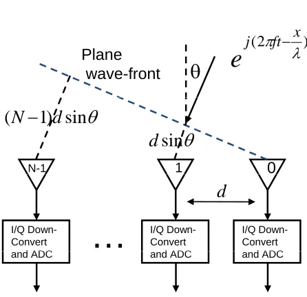
To avoid mechanically rotating the antenna, we can use a technology calledbeamformingwhich allowed us to change the beampattern electronically. This requires multiple antennas and usually these antennas have wider beampatterns. For convenience, we assume the antennas all have om-nidirectional beampatterns. In other words, for every antenna, B(θ) = 1for allθ. The multiple antennas are placed uniformly on a straight line. This is called a uniform linear antenna array (ULA). Fig. 1.8 illustrates such an antenna array. Consider a narrowband plane wave with carrier frequencyfcimpinging from angleθ. The received signal of thenth antenna can be expressed as

rn(t) =αs(t)ej 2π

λdnsinθ+v(t),

forn= 0,1,· · ·, N−1,whereN is the number of antennas,λ= c

fc is the wavelength of the signal,

s(t)is the signal envelope,αis the amplitude response andv(t)is the additive noise. The phase difference termej2π

)

2

(

λ

π

ft

x

j

e

−

Plane

wave-front

θ

0

θ

sin

d

θ

sin

)

1

(

N

−

d

N-1 I/Q Down-Convert d ADC I/Q Down-Convert d ADC I/Q Down-Convert d ADC

…

d

and ADC and ADC and ADC

Figure 1.8: A uniform linear antenna array (ULA)

in Fig. 1.8. To extract signal fromθ, one can linearly combine the received signals and obtain

y(t) =

N−1

X

n=0

wnrn(t)

= αs(t)

N−1

X

n=0

wnej 2π

λdnsinθ

| {z }

B(θ)

+

N−1

X

n=0

wnv(t), (1.3)

wherewnis the weighting coefficient corresponding to thenth antenna. Observing the above

equa-tion, one can see thaty(t)has a different gain for signal coming from different angleθ. Therefore by linearly combining the signals, we can synthesize the beampatternB(θ)as shown in Eq. (1.3). Note that this beampatternB(θ)can be controlled by the weighting coefficientswn.

To change the beampattern, we do not need to mechanically rotate the antenna. We can just change the weighting coefficientswn and this can be done through using electronic devices. This

technique is called electric beamforming and the weighting coefficientswn are calledbeamformer

coefficients. The beampattern can be expressed as

B(θ) =

N−1

X

n=0

wnej 2π

λdnsinθ

=

N−1

X

n=0

wne−jωn

_ω=2π

λdsinθ

= W(ejω)_ω=2π

whereW(ejω)is the Fourier transform of the beamformerwn. Therefore, the beamformer design

problem can be treated as an FIR filter design problem. Typical FIR filter design algorithms such as Parks-McClellan algorithm can be applied to beamformer design. Note that in filter design problem, the frequency resolution of a filter depends on the filter order. Similarly, the spatial reso-lution of the beamformer depends on the number of antennas in the ULA array. Note that we have

ω = 2_λπdsinθin the above equation. Ifd > λ₂, there will be multiple values ofθ mapping to the sameω. This is equivalent to the aliasing effect in sampling. To avoid this, one choosesd≤ λ

2. In practice, the spacing between antennas is about half of the wavelength. In this case,

−π≤ω=2π

λ dsinθ=πsinθ≤π.

Then there will not be aliasing in the beampattern. Beamforming has long been used in many areas, such as radar, sonar, seismology, medical imaging, speech processing, and wireless commu-nications. We will talk more about beamforming in Chapter 2.

1.2

Review of MIMO Radar

In the traditional phased array radar, the system can only transmit scaled versions of a single wave-form. Because only a single waveform is used, the phased array radar is also called SIMO (single-input multiple-output) radar in contrast to the MIMO radar. We will use “SIMO radar” or “phased array radar” alternatively throughout the thesis.

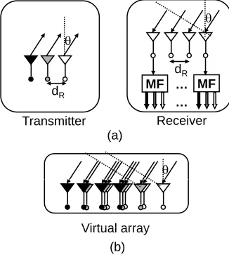
colocated such that the RCS observed by each transmitting path are identical. The components extracted by the matched filters in each receiving antenna contain the information of a transmitting path from one of the transmitting antenna elements to one of the receiving antenna elements. By using the information about all of the transmitting paths, a better spatial resolution can be obtained. The phase differences caused by different transmitting antennas along with the phase differences caused by different receiving antennas can form a newvirtual arraysteering vector. With judiciously designed antenna positions, one can create a very long array steering vector with a small number of antennas. Thus the spatial resolution for clutter can be dramatically increased at a small cost [7,85]. We will soon introduce the virtual array concept. It has been shown that this kind of radar system has many advantages such as excellent clutter interference rejection capability [15, 75], improved parameter identifiability [67], and enhanced flexibility for transmitting beampattern design [37,94]. Some of the recent work on the colocated MIMO radar has been reviewed in [66]. In this chapter, we focus on the colocated MIMO radar.

1.2.1

The Virtual Array Concept

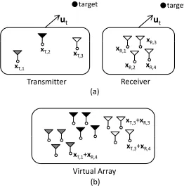
One of the main advantages of MIMO radar is that the degrees of freedom can be greatly increased by the concept of virtual array. In this section, we briefly review this concept. More detailed reviews can be found in [7, 32, 85, 88]. Consider an arbitrary transmitting array withM antenna elements and an arbitrary receiving array withNantenna elements. Themth transmitting antenna is located atxT ,m ∈R3and thenth receiving antenna is located atxR,n ∈R3. Fig. 1.9 (a) shows an example

withM = 3andN = 4. Themth transmitting antenna emits the waveformφm(t). The emitted

waveforms are orthogonal, that is,

Z

φm(τ)φ∗k(τ)dτ =δmk.

In each receiving antenna, these orthogonal waveforms are extracted byM matched filters. There-fore, the total number of extracted signals equalsN M. Consider a far-field point target. The target response in themth matched filter output of thenth receiving antenna can be expressed as

y(_n,mt) =ρtexp(j

2π

λu

T

x

u

u

target

target

x

x

x

x

x

x

x

Transmitter

Receiver

( )

x

+

x

(a)

x

+

x

x

+

x

Virtual

Array

(b)

( )

where ut ∈ R3 is a unit vector pointing toward the target from the radar station, and ρt is the

amplitude of the signal reflected by the target. One can see that the phase differences are created by both the transmitting antenna locations and the receiving antenna locations. The target response in (1.4) is the same as the target response received by a receiving array withN Mantenna elements located at

{xT ,m+xR,n|n= 0,1,· · ·, N−1, m= 0,1,· · ·, M −1}.

We call thisN M-element array avirtual array. Fig 1.9 (b) shows the corresponding virtual array of the MIMO radar system illustrated in (a). Thus, we can create anN M-element virtual array by using onlyN+Mphysical antenna elements.

The relation between the transmitting array, receiving array, and the virtual array can be further characterized by a convolution [32]. Define

gT(x) = M−1

X

m=0

δ(x−xT ,m) (1.5)

and

gR(x) = N−1

X

n=0

δ(x−xR,n). (1.6)

These functions characterize the antenna locations in the transmitter and receiver. Because the virtual array hasN Mvirtual elements located at{xT ,m+xR,n}, the corresponding function which

characterizes the antenna location of the virtual array can be expressed as

gV(x) = M−1

X

m=0

N−1

X

n=0

δ(x−(xT ,m+xR,n)). (1.7)

Comparing (1.5)–(1.7), one can see that

gV(x) = (gT ∗gR)(x), (1.8)

where∗denotes convolution. One can observe this relation from Fig. 1.9. The array in Fig. 1.9 (b) can be obtained by performing convolution of the arrays in Fig. 1.9 (a). This relation was observed in [32].

system, the overall beampattern is the product of the transmit and receive beampatterns. The overall beampattern is therefore related to a weight vectorwtrwhich equals the convolution of the

transmit beamformerwtand the receive beamformerwr. That is

wtr =wt∗wr. (1.9)

This new weight vectorwtr can be viewed as a beamformer of a longer array called coarray. In

terms of the array geometry, this coarray is exactly the virtual array. However, these two ap-proaches are completely different due to the difference between SIMO and MIMO systems. In the MIMO virtual array, the weight vector has a total of N M degrees of freedom. However, in coarray, the weight vector has onlyN +M degrees of freedom because of (1.9). Also, the virtual array beamforming is performed in the receiver only, but the coarray beamforming is performed in the both sides of the transmitter and receiver.

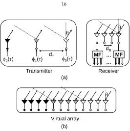
EXAMPLE 1.1: Uniform Linear Virtual Array. Consider the a MIMO radar system with the

uniform linear arrays (ULA) in both of the transmitter and the receiver. In this case, the antenna locationsxT ,mandxR,nreduce to scalars and

xR,n=ndR, n= 0,1,· · ·, N−1

xT ,m =mdT, m= 0,1,· · ·, M−1,

wheredRis the spacing between the receiving antennas, anddT is the spacing between the

trans-mitting antennas. Fig. 1.10 shows an example withM = 3andN = 4. Similar to the arbitrary antenna case, the target response in the mth matched filter of thenth receiving antenna can be expressed as

ρtexp(j

2π

λ (ndRsinθ+mdTsinθ)), (1.10)

whereθis the looking direction of the target. The phase differences are created by both transmitting and receiving antenna locations. Define

fs,

dR

λ sinθ, andγ, dT

dR

θ

θ

d

d

MF

MF

Transmitter

Receiver

d

φ

(τ)

φ

(τ)

φ

(τ)

MF

…

MF

…

θ

(a)

θ

Virtual array

(b)

Figure 1.10: (a) A ULA MIMO radar system withM = 3andN = 4. (b) The corresponding virtual array

Equation (1.10) can be further simplified as

ρtexp(j2πfs(n+γm)).

If we choose

γ=N, (1.11)

domain, a better spatial resolution can be obtained.

EXAMPLE 1.2: Overlapped Linear Virtual Array. Instead of choosingγ =N in (1.11), one

can chooseγ = 1. In this case, the target response in themth antenna of thenth receiver can be expressed as

ρtexp(j2πfs(n+m)).

Fig. 1.11 shows an example of the transmitter, receiver and their corresponding virtual array. In

θ

θ

dR

MF MF

θ

Transmitter Receiver

MF … MF …

( ) dR

(a)

θ

Virtual array Virtual array

(b)

Figure 1.11: (a) A MIMO radar system withM = 3,N = 4anddT =dR. (b) The corresponding

virtual array

this case, the virtual array is more complicated: It has several virtual elements which are at the same locations. In some sense, we can regard this as a nonuniform virtual array. The advantage of choosingγ= 1is that the radar station can form a focused beam by emitting correlated waveforms {φm(t})[37]. The transmit beamforming can not be done in the caseγ=N, because the sampling

rate in the spatial domain is too low to prevent aliasing. However, the advantage of choosingγ=N

is that the virtual array is longer as shown in Fig. 1.10 (b) which results in a better spatial resolution.

1.3

Outline of the Thesis

algorithm for space-time adaptive processing in MIMO radar. The relevant results have been pub-lished in [15] and Chapter 6 of [70]. Chapter 4 and Chapter 5 study the transmitted waveform in MIMO radar. Chapter 4 introduces the MIMO ambiguity function and uses it to design the trans-mitted waveforms. The corresponding waveforms result in a good resolution for point targets. The result in Chapter 4 has been published in [16]. In Chapter 5, the waveform is optimized using the prior information about the target and clutter. Also, the corresponding receiving filter is jointly optimized to achieve better SINR performance. The result in Chapter 5 can be found in [18]. We will briefly explain the major results of each chapter in this section.

1.3.1

Robust Beamforming — Chapter 2

1.3.2

Efficient Space-Time Adaptive Processing — Chapter 3

We have explained Doppler processing in Section 1.1.2 and beamforming in Section 1.1.3. Space-time adaptive processing (STAP) is the combination of both Doppler processing and beamforming. It linearly combines all the antenna outputs from different slow time indexes. The STAP is usually used in airborne radar. This is because the Doppler frequency of the ground clutter depends on the looking angle. Therefore in airborne radar the Doppler and angle information has to be jointly pro-cessed. Joint processing signals of two dimensions requires much more computational complexity. There have been many algorithms proposed in [35, 40, 43–45, 57, 105] and the references therein for improving the complexity and convergence of the STAP in the SIMO radar.

Using MIMO radar improves the angle resolution of the STAP. However, MIMO radar also increases the signal dimension by adding the new waveform-dimension. Therefore it requires more computational complexity. Furthermore, it requires more signal samples to estimate the second order statistics when the dimension of the signal is large. In Chapter 3, we propose an algorithm which fully uses the geometry of the problem and the characteristics of the covariance matrices. The proposed method has a significantly lower computational complexity and requires fewer training signal samples.

1.3.3

Ambiguity Function and Waveform Design — Chapter 4

We have discussed range resolution and pulse compression in Section 1.1.1. In fact the overall radar resolution combines range resolution, Doppler resolution and angle resolution. The overall resolution can be characterized by the radar ambiguity function. The radar ambiguity function is defined as the system response to a point target. A sharp radar ambiguity function implies the system has a good resolution to point targets. The ambiguity function is determined by the radar transmitted waveform. It is the major tool for analyzing the radar waveform. The radar ambiguity function has been extended to the MIMO case in [89].

linear frequency modulation waveforms.

1.3.4

Joint Transmitted Waveform and Receiver Design — Chapter 5

In Chapter 5, we consider joint transmitted waveform and receiver design with some prior infor-mation of the extended target and clutter. While the waveform design problem in Chapter 4 is optimal for point targets, the waveform design problem in Chapter 5 is for the extended target. An extended target can be viewed as a collection of infinite number of point targets. It can be character-ized with a certain impulse response. The single-input single-output (SISO) version of this problem has been studied by DeLong and Hofstetter in 1967 [22–24] and more recently by Pillai et al. [82]. Different iterative methods have been proposed. In Chapter 5, we consider the MIMO extension of this problem. In the MIMO case, the method proposed in [22] cannot be applied because it is based on the symmetry property of the SISO radar ambiguity function. The method in [82] can still be applied to the MIMO case. However, this method does not guarantee the SINR to be nondecreasing in each iteration step. We propose a new iterative algorithm which can be applied to the MIMO case while guaranteeing the SINR to be nondecreasing in each iteration step. The corresponding iterative algorithms are also developed for the case where only the statistics or the uncertainty set of the target impulse response is available. These algorithms guarantee that the SINR performance improves in each iteration step. Numerical results show that the proposed methods have better SINR performance than existing design methods.

1.4

Notations

In this section, we define the notations used in this thesis. Matrices and vectors are denoted by capital letters in boldface (e.g.,A). SuperscriptT_and†_{denote transpose and transpose conjugation}

respectively. The expression(A)k,lrepresents the element of matrixAlocated at thekth row and

thelth column. The notation diag(A,A,· · ·,A)denotes a block diagonal matrix whose diagonal blocks areA. The notation tr(A)denotes the trace of matrixA. The notationkAkF denotes the

Frobenius norm of the matrixA. The notation ]adenotes the angle of the complex numbera. The notationbacis defined as the largest integer smaller thana. The notationdaeis defined as the smallest integer larger thana. The notation(n modm)represents the remainder of division ofn

matrixA∈ CN×M_{, thekth element of the vectorx=vec(A)∈ C}N M×1_{can be expressed as}

(x)k= (A)(k modN),bkc.

Chapter 2

Robust Beamforming

This chapter focuses on robust beamforming algorithms. We have briefly talked about beamform-ing in Chapter 1. Beamformers can be designed accordbeamform-ing to the statistics of the received signals to optimize for the system SINR (signal to interference plus noise ratio). It is well known that the performance of such a beamformer is very sensitive to direction-of-arrival (DOA) errors. In MIMO radar, the virtual array can be much larger than the physical receiving array in the SIMO radar. Therefore the robustness of the beamformer becomes even more important in the MIMO radar case.

In this chapter, an adaptive beamformer that is robust against the DOA mismatch is proposed. This method imposes two quadratic constraints such that the magnitude responses of two steering vectors exceed unity. Then a diagonal loading method is used to force the magnitude responses at the arrival angles between these two steering vectors to exceed unity. Therefore this method can always force the gains at a desired range of angles to exceed a constant level while suppressing the interferences and noise. A closed form solution to the proposed minimization problem is intro-duced, and the diagonal loading factor can be computed systematically by a proposed algorithm. Numerical examples show that this method has an excellent SINR performance and a complexity comparable to the standard adaptive beamformer. Most of the results of this chapter have been reported in our recent journal paper [14].

2.1

Introduction

unity and minimizes the variance of the beamformer output. This method is called minimum vari-ance distortionless response (MVDR) beamformer in the literature. The MVDR beamformer has very good resolution, and the SINR (signal-to-interference-plus-noise ratio) performance is much better than traditional data-independent beamformers. However, when the steering vector of the SOI is imprecise, the response of the SOI is no longer constrained to be unity and is thus attenuated by the MVDR beamformer while minimizing the total variance of the beamformer output [20]. The effect is called signal cancellation. It dramatically degrades the output SINR. A good introduction to this topic can be found in [64]. The steering vector of the SOI can be imprecise because of various reasons such as direction-of-arrival (DOA) errors, local scattering, near-far spatial signature mis-match, waveform distortion, source spreading, imperfectly calibrated arrays and distorted antenna shape [64], [44]. In this chapter, we focus on DOA uncertainty.

There are many methods developed for solving the DOA mismatch problem. In [4, 8, 11, 26, 31, 96, 98, 103], linear constraints have been imposed when minimizing the output variance. The linear constraints can be designed to broaden the main beam of the beampattern. These beamformers are called linearly constrained minimum variance (LCMV) beamformers. In [84] and [99], convex quadratic constraints have been used. In [6], a Bayesian approach has been used. For other types of mismatches, diagonal loading [1, 13] is known to provide robustness. However, the drawback of the diagonal loading method is that it is not clear how to choose a diagonal loading factor. In [27], the steering vector has been projected onto the signal-plus-interference subspace to reduce the mismatch. In [107], the magnitude responses of the steering vectors in a polyhedron set are constrained to exceed unity while the output variance is minimized. This method avoids the signal cancellation when the actual steering vector is in the designed polyhedron set. In [102], Vorobyov et al. have used a non-convex constraint which forces the magnitude responses of the steering vectors in a sphere set to exceed unity. This non-convex optimization problem has been reformulated in a convex form as a second order cone programming (SOCP) problem. It has been also proven in [102] that this beamformer belongs to the family of diagonal loading beamformers. In [63,73], the sphere uncertainty set has been generalized to an ellipsoid set and the SOCP has been avoided by the proposed algorithms which efficiently calculate the corresponding diagonal loading level. In [91], a general rank case has been considered using similar idea as in [102] and an elegant closed form solution has been obtained.

been forced to exceed unity while minimizing the output variance. The uncertainty set has been selected as polyhedron, sphere, or ellipsoid in order to be robust against general types of steering vector mismatches. In this chapter, we consider only the DOA mismatch. Inspired by these un-certainty based methods, we consider a simplified unun-certainty set which contains only the steering vectors with a desired uncertainty range of DOA. To find a suboptimal solution for this problem, the constraint is first loosened to two non-convex quadratic constraints such that the magnitude responses of two steering vectors exceed unity. Then a diagonal loading method is used to force the magnitude responses at the arrival angles between these two steering vectors to exceed unity. Therefore this method can always force the gains at a desired range of angles to exceed a constant level while suppressing the interferences and noise. A closed form solution to the proposed min-imization problem is introduced, and the diagonal loading factor can be computed systematically by a proposed iterative algorithm. Numerical examples show that this method has an excellent SINR performance and a complexity comparable to the standard MVDR beamformer.

The rest of the chapter is organized as follows: The MVDR beamformer and the analysis of steering vector mismatch are presented in Section 2.2. Some previous work on robust beamforming is reviewed in Section 2.3. In Section 2.4, we develop the theory and the algorithm of our new robust beamformer. Numerical examples are presented in Section 2.5. Finally, the conclusions are presented in Section 2.6.

2.2

MVDR Beamformer and the Steering Vector Mismatch

Consider a uniform linear array (ULA) ofN omnidirectional sensors with interelement spacingd. The signal of interest (SOI) is a narrowband plane wave impinging from angleθ. The baseband array outputy(t)can be expressed as

y(t) = x(t)s(θ) +v(t),

wherev(t)denotes the sum of the interferences and the noises,x(t)is the signal of interest (SOI), ands(θ)represents the baseband array response of the SOI. It is called steering vector and can be expressed as

s(θ) _, 1 ej2λπdsinθ · · · ej(N−1) 2π

λdsinθ

T

whereλis the operating wavelength. The output of the beamformer can be expressed asw†y(t),

where w is the complex weighting vector. The output SINR (signal-to-interferences-plus-noise ratio) of the beamformer is defined as

SINR,E|x(t)w †_s(θ)|2

E|w†_v(t)|2 =

σ2

x|w†s(θ)|2

w†_R

vw

, (2.2)

whereRv ,E[v(t)v†(t)], andσx2 ,E[|x(t)|2]. By varying the weighting factors the output SINR

can be maximized by minimizing the total output variance while constraining the SOI response to be unity. This can be written as the following optimization problem:

min

w w

†_R

yw

subject tos†(θ)w= 1, (2.3)

whereRy,E[y(t)y†(t)].This is equivalent to minimizingw†Rvwsubject to|s†(θ)w|= 1because

w†Ryw = w†Rvw+σx2|s

†_(θ)w|2

= w†Rvw+σx2·1.

The solution to this problem is well-known and was first given by Capon in [12] as

wc=

Ry−1s(θ)

s†_(θ)R

y−1s(θ)

. (2.4)

This beamformer is called minimum variance distortionless response (MVDR) beamformer in the literature. When there is a mismatch between the actual arrival angleθand the assumed arrival angleθm, this beamformer becomes

wm=

Ry−1s(θm)

s†_(θ

m)Ry−1s(θm)

. (2.5)

It can be viewed as the solution to the minimization problem

min

w w

†_R

yw

Becausew†Ryw=w†Rvw+σx2|s†(θ)w|2, ands†(θ)w= 1is no longer valid due to the mismatch,

the SOI magnitude response might be attenuated as a part of the objective function. This suppres-sion leads to severe degradation in SINR, because the SOI is treated as a interference in this case. The phenomenon is called signal cancellation. A small mismatch can lead to a severe degradation in the SINR.

2.3

Previous Work On Robust Beamforming

Many approaches have been proposed for improving the robustness of the standard MVDR beam-former. In this section, we briefly mention some of them related to our work.

2.3.1

Diagonal Loading Method

In [1, 13], the optimization problem in Eq. (2.3) is modified as

min

w w

†_(R

y+γIN)w

subject tos†(θ)w= 1,

2.3.2

LCMV Method

In [4, 8, 11, 26, 31, 96, 98, 103], the linear constraint of the MVDR in Eq. (2.3) has been generalized to a set of linear constraints as

min

w w

†_R

yw

subject toC†w=f, (2.7)

whereC†is anL×Nmatrix andf is anL×1vector. The solution can be found by using Lagrange multiplication method as

wl=Ry−1C(C†Ry−1C)−1f.

This is called the linearly constrained minimum variance (LCMV) beamformer. These linear con-straints can be directional concon-straints [96, 103] or derivative concon-straints [4, 11, 26]. The directional constraints force the responses of multiple neighbor steering vectors to be unity. The derivative constraints force not only the response to be unity but also several orders of the derivatives of the beampattern in the assumed DOA to be zero. These constraints broaden the main beam of the beampattern so that it is more robust against the DOA mismatch. In [98], linear constraints have further been used to allow an arbitrary specification of the quiescent response.

2.3.3

Extended Diagonal Loading Method

In [102], the following optimization problem is considered.

min

w w

†_R

yw

subject to|w†s| ≥1,∀s∈ E, (2.8)

whereEis a sphere defined as

E={¯s+e

kek ≤}, (2.9)

in [102], it is reformulated to a second order cone programming (SOCP) problem which can be solved by using some existing tools such as SeDuMi in MATLAB. It has also been proven in [102] that the solution to Eq. (2.8) has the formc(Ry+γIN)−1¯sfor some appropriatecandγ. Therefore

this method can be viewed as an extended diagonal loading method [63]. In [63,73], the uncertainty set in Eq. (2.9) has been generalized to an ellipsoid and the SOCP has been avoided by the proposed algorithms which directly calculate the corresponding diagonal loading levelγas a function ofRy,

¯

sand.

2.3.4

General-Rank Method

In [91], a general-rank signal model is considered. The steering vectorsis assumed to be a random vector that has a covarianceRs. The mismatch is therefore modeled as an error matrix∆1∈CN×N in the signal covariance matrixRsand an error matrix∆2∈CN×Nin the output covariance matrix

Ry. The following optimization problem is considered:

min

w k∆max2kF≤γ

w†(Ry+∆2)w

subject tow†(Rs+∆1)w≥1∀ k∆1kF ≤,

wherek∆kF denotes the Frobenius norm of the matrix∆, andandγare the upper bounds of the

Frobenius norms of the error matrices∆1and∆2, respectively. This optimization problem has an elegant closed form solution as shown by Shahbazpanahi et al. in [91], namely,

wn=P{(Ry+γIN)−1(Rs−IN)}, (2.10)

whereP{A}denotes the principal eigenvector of the matrixA. The principal eigenvector is defined as the eigenvector corresponding to the largest eigenvalue.

2.4

New Robust Beamformer

This optimal robust beamformer problem can be expressed as

wd= arg min

w w

†_R

yw

subject to|s†(θ)w|2_≥1

forθ1≤θ≤θ2, (2.11)

whereθ1andθ2are the lower and upper bounds of the uncertainty of SOI arrival angle respectively, ands(θ)is the steering vector defined in Eq. (2.1) with the arrival angleθ. The following uncertainty set of steering vectors is considered:

{s= 1 ejω _{· · · e}j(N−1)ω T

ω1≤ω≤ω2}, (2.12)

where ω1 , 2πsinθ1/λ, andω2 , 2πsinθ2/λ. This uncertainty set is a curve. This constraint protects the signals in the range of anglesθ1≤θ≤θ2from being suppressed.

2.4.1

Frequency Domain View of the Problem

Substituting Eq. (2.12) into the constraint in Eq. (2.11), the constraint can be rewritten as

N−1

X

n=0

wne−jωn

=|W(ejω)| ≥1forω1≤ω≤ω2,

whereW(ejω_{)is the Fourier transform of the weight vectorw. The objective functionw}†_R

ywcan

also be rewritten in the frequency domain as

w†Ryw =

N−1

X

n=0

N−1

X

m=0

w∗nRy,n,mwm

=

N−1

X

n=0

N−1

X

m=0

w∗_nry(n−m)wm

= 1

2π Z 2π

0

|W(ejω)|2_S

y(ejω)dω,

whereSy(ejω)is the power spectral density (PSD) of the array outputy. Therefore, the optimization

problem can be rewritten in the frequency domain as

min

w

Z 2π

0

|W(ejω)|2_S

y(ejω)dω

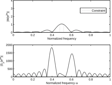
Note thatSy(ejω) is a weighting function in the above integral. The frequency domain view of

this optimization problem is illustrated in Fig. 2.1. The integral of|W(ejω_)|2_S

y(ejw)is minimized

0 0.2 0.4 0.6 0.8 1

0 1 2 3 4

|W(e

jω)|

Normalized frequency

Constraint

0 0.2 0.4 0.6 0.8 1

0 500 1000 1500 2000

|Sy

(e

jω)|

Normalized frequency ω

Figure 2.1: Frequency domain view of the optimization problem

while|W(ejω_{)| ≥1forω}

1≤ω ≤ω2is satisfied. Even though we will not solve the problem in the frequency domain, it is insightful to look at it this way.

2.4.2

Two-Point Quadratic Constraint

It is not clear how to solve the optimal beamformerwdin Eq. (2.11) because the constraint does

not fit into any of the existing standard optimization methods. The constraint|s†(θ)w|2 _{≥ 1 for}

θ1 ≤ θ ≤ θ2 can be viewed as infinite number of non-convex quadratic constraints. To find a suboptimal solution, we start looking for the solution by loosening the constraint. We first loosen the constraint by choosing only two constraints|s†(θ1)w|2≥1and|s†(θ2)w|2≥1from the infinite constraints|s†(θ)w|2_≥1forθ

1≤θ≤θ2. The corresponding optimization problem can be written as

min

w w

†_R

yw

subject to|s†(θ1)w|2≥1, and|s†(θ2)w|2≥1. (2.13)

equivalent form:

min

w,φ,ρ0≥1,ρ1≥1

w†Ryw

subject toS†w= 

 ρ0

ρ1ejφ



,

where

S= s(θ1) s(θ2)

,

andρ0,ρ1, andφare real numbers.

To solve this problem, we divide it into two parts. We first assumeφ,ρ0, andρ1are constants and solvew. The solutionwwill be a function ofφ,ρ0, andρ1. Then the solutionwcan be substituted back into the objective function so that the objective function becomes a function ofφ,ρ0, andρ1. Finally, we minimize the new objective function by choosingφ,ρ0, andρ1. Define the function

L(w,b) =w†Ryw−b†S†w, (2.14)

whereb∈C2_{is the Lagrange multiplier. Taking the gradient of Eq. (2.14) and equating it to zero,} we obtain the solution

w0=Ry−1Sb.

Substituting the above equation into the constraint, the Lagrange multiplier can be expressed as

b= (S†Ry−1S)−1



 ρ0

ρ1ejφ



.

Substitutingbback intow0, we obtain

w0=Ry−1S(S†Ry−1S)−1



 ρ0

ρ1ejφ



. (2.15)

However, this approach is reformulated from the non-convex quadratic problem in Eq. (2.13). It is intrinsically different from a linearly constrained problem. The task now is to solve forφ,ρ0, and

ρ1. Write

(S†Ry−1S)−1=





r0 r2ejβ

r2e−jβ r1



,

wherer0,r1, andr2are real nonnegative numbers. Substitutingw0in Eq. (2.15) into the objective function, it becomes

w†₀Ryw0 =

ρ0 ρ1e−jφ

(S†Ry−1S)−1



 ρ0

ρ1ejφ





= r0ρ20+r1ρ21+ 2Re{r2ρ0ρ1ej(β+φ)}

≥ r0ρ20+r1ρ12−2r2ρ0ρ1. (2.16)

To minimize the objective function,φcan be chosen as

φ=−β+π (2.17)

so that the last equality in Eq. (2.16) holds. Nowφandw0are obtained by Eq. (2.17) and Eq. (2.15), and the objective function becomes Eq. (2.16). To further minimize the objective function,ρ0, and

ρ1can be found by solving the following optimization problem:

min

ρ0≥1, ρ1≥1

r0ρ20+r1ρ12−2r2ρ0ρ1.

This can be solved by using the Karush-Kuhn-Tucker (KKT) condition. The following solution can be obtained:

ρ0 =

 



1, r2/r0≤1

r2/r0, r2/r0>1

,

ρ1 =

 



1, r2/r1≤1

r2/r1, r2/r1>1

. (2.18)

Algorithm 1 Givenθ1,θ2, andRy, computew0by the following steps:

1. S← s(θ1) s(θ2)

.

2. V←(Ry)−1S.

3. R_,





r0 r2ejβ

r2e−jβ r1



←(S

†_V)−1_.

4. φ← −β+π.

ρ0←

 



1, r2/r0≤1

r2/r0, r2/r0>1

.

ρ1←

 



1, r2/r1≤1

r2/r1, r2/r1>1

.

5. w0←VR



 ρ0

ρ1ejφ



.

The matrix inversion in Step 2 contains most of the complexity of the algorithm. Therefore the algorithm has the same order of complexity as the MVDR beamformer. Because the constraint is loosened, the feasible set of the two-point quadratic constraint problem in Eq. (2.13) is a superset of the feasible set of the original problem in Eq. (2.11). The minimum found in this problem is a lower bound of the minimum of the original problem. If the solution w0 in the two-point quadratic constraint problem in Eq. (2.13) happens to satisfy the original constraint|s†(θ)w0|2_≥1 forθ1 ≤θ≤θ2, thenw0is exactly the solution to the original problem in Eq. (2.11). The example provided in Fig. 2.1 is actually found by using the two-point quadratic constraint instead of the original constraint, but it also satisfies the original constraint. This makes it exactly the solution to the original problem in Eq. (2.11).

Unfortunately, in general the original constraint|s†_{(θ)w| ≥1forθ}

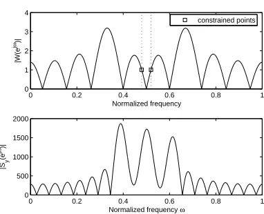
1≤θ≤θ2is not guaranteed to be satisfied by the solution of the two-point quadratic constraint problem in Eq. (2.13). Fig. 2.2 shows an example where the original constraint is not satisfied. This example is obtained by increasing the power of the SOI in the example in Fig. 2.1. One can compare|Sy(ejω)|in Fig. 2.1

and Fig. 2.2 and find that the SOI power is much stronger in Fig. 2.2. In this case, the beamformer tends to put a zero betweenθ1andθ2to suppress the strong SOI. This makes|W(ejω)| ≤1for some

0 0.2 0.4 0.6 0.8 1 0

1 2 3 4

|W(e

jω)|

Normalized frequency

constrained points

0 0.2 0.4 0.6 0.8 1

0 500 1000 1500 2000

|Sy

(e

jω)|

Normalized frequency ω

Figure 2.2: Example of a solution of the two-point quadratic constraint problem that does not satisfy |s†w| ≥1forθ1≤θ≤θ2

2.4.3

Two-Point Quadratic Constraint with Diagonal Loading

In Fig. 2.2, we observe that the energy ofw,kwk2 ₌ R2π

0 |W(e

jω_)|2_{dω/(2π) is quite large} com-pared to that in Fig. 2.1. Fig. 2.3 shows the locations of the zeros of the z-transformW(z)of the beamformer in Fig. 2.2. One can observe that there is a zero betweenθ1andθ2. This zero causes

−1 −0.5 0 0.5 1

−1 −0.8 −0.6 −0.4 −0.2 0 0.2 0.4 0.6 0.8

1 constrained points

zeros

Figure 2.3: The locations of zeros of the beamformer in Fig. 2.2

the signal cancellation in Fig. 2.2. It can be observed that the zero is very close to those two points which are constrained to have magnitudes greater than unity. When a zero is close to these quadrat-ically constrained points, it attenuates the gain at these points. However, the magnitude responses at these points are constrained to exceed unity. To satisfy the constraints, the overall energy ofw

Fig. 2.3, the norm of the weighting vectorkwkwill become very large. By using this fact, we can impose some penalty onkwk2_{to force the zeros betweenθ}

1andθ2to go away. This can be done by the diagonal loading approach mentioned in Sec. 2.3.1. The corresponding optimization problem can be written as

wγ = arg min

w w

†_R

yw+γkwk2

subject to|s†(θ1)w| ≥1, and|s†(θ2)w| ≥1, (2.19)

whereγis the diagonal loading factor which represents the amount of the penalty put onkwk2_. The solutionwγ can be found by performing the following modification on the output covariance

matrix:

Ry←Ry+γIN

and then applying Algorithm 1. Whenγ→ ∞, the solution converges to

w∞= arg min

w kwk

2

subject to|s†(θ1)w| ≥1, and|s†(θ2)w| ≥1. (2.20)

The following lemma gives the condition for whichw∞satisfies the constraint|s(θ)†w∞| ≥ 1for

allθinθ1≤θ≤θ2.

Lemma 1 |s†(θ)w∞| ≥1forθ1≤θ≤θ2if and only if|sinθ2−sinθ1| ≤λ/(dN).

Proof:According to Eq. (2.20), substitutingRy=IN and applying Algorithm 1, one can obtain

w∞=

1 N+|sincd(ω2−ω1

2 )|

(s(θ1) +s(θ2)ej

(ω2−ω1 )(N−1) 2 ),

where

ω1,

2π

λdsinθ1, ω2, 2π

λdsinθ2, and

By direct substitution, one can obtain

|s†(θ)w∞|=

sincd(ω1−ω

2 ) +a·sincd(

ω2−ω 2 )

N+|sincd(ω2−ω1 2 )|

, (2.21)

whereω_,2_λπdsinθand

a=

 



1 , if sincd(ω2−ω1 2 )>0

−1 , otherwise. By Eq. (2.21), it can be verified that

|s†(θ)w∞| ≥1forω1≤ω≤ω2

if and only if

|ω2−ω1| ≤

2π N

which can also be expressed as|sinθ2−sinθ1| ≤λ/(dN).

If the condition|sinθ1−sinθ2| ≤λ/(dN)is satisfied, there exists aγ >0such that the condition |s†(θ)wγ| ≥1forθ1≤θ≤θ2is satisfied. For example, ifd=λ/2,N = 10,θ1 = 35◦andθ2 = 55◦ then we have

|sin(55◦)−sin(35◦)| ≈0.1824≤ λ

dN = 0.2.

In this case, there exists a γ > 0so that the robust condition |s†_(θ)w

γ| ≥ 1 for 35◦ ≤ θ ≤ 55◦

is satisfied. However, introducing the diagonal loading changes the objective functionw†Rywto

w†(Ry+γIN)w. The modification of the objective function affects the suppression of the

inter-ferences. To keep the objective function correct,γshould be chosen as small as possible while the condition|s†(θ)w| ≥1forθ1 ≤θ≤θ2is satisfied. For finding such aγ, we propose the following algorithm:

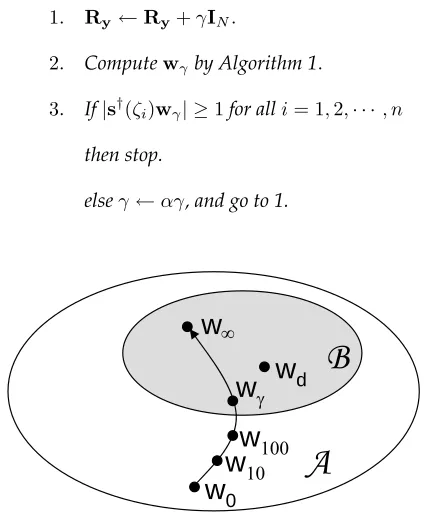
1,2,· · · , nwhich satisfiesθ1< ζi< θ2for alli,wγcan be computed by the following steps:

1. Ry←Ry+γIN.

2. Computewγ by Algorithm 1.

3. If|s†(ζi)wγ| ≥1for alli= 1,2,· · · , n then stop.

elseγ←αγ, and go to 1.

w

w

w

w

w

w

f

A

B

Figure 2.4: An illustration of Algorithm 2, where A = {w|s†(θ)w| ≥ 1, θ = θ1, θ2} and B = {w|s†(θ)w| ≥1, θ1≤θ≤θ2}

Fig. 2.4 illustrates how Algorithm 2 works. In this figure, the setA = {w|s†(θ)w| ≥ 1, θ = θ1, θ2}is the feasible set of the two-point quadratic constraint problem in Eq. (2.13). The setB= {w|s†(θ)w| ≥1, θ1≤θ≤θ2}is the feasible set of the mismatched steering vector problem in Eq. (2.11). If the condition|sinθ1−sinθ2| ≤λ/(dN)is satisfied, Lemma 1 shows thatw∞∈ B. In this

case, there exists aγ >0so thatwγ ∈ B. Algorithm 2 keeps increasingγby multiplyingαuntil

|s†(ζi)wγ| ≥1for alli= 1,2,· · ·, nis satisfied. This is an approximation forwγ ∈ B.The number

ncan be very small. In the next section,n = 3works well for all the cases. Also the SINR is not sensitive to the choice ofα, as we will see later.

2.5

Numerical Examples

For the purpose of design examples, the same parameters used in [73] are used in this section. An un