Evaluation of Equity in the Cadaver Kidney
Allocation System- A Case Study from India
Pius Tom1, Dr. K Sunil Kumar2, Dr. Noble Gracious3
P.G. Research Scholar, Department of Mechanical Engineering, College of Engineering Trivandrum, Kerala, India1
Associate Professor, Department of Mechanical Engineering, College of Engineering Trivandrum, Kerala, India2
Nodal Officer, Kerala Network for Organ Sharing, Kerala, India3
ABSTRACT: Cadaver kidney transplantation requires the selection of a recipient from a large pool of patients waiting
across various geographic zones, making the process challenging and complex. For improving efficiency of transplantation, the selection has to be made from a pool of recipients waiting in the same allocation zone as that of the identified donor. Equity issues often arise due to geographic disparity in the allocation system. Many deserving patients fail to get a kidney on time because they are in the wrong geographic zone. This work evaluates the geographic disparity issues in one of the states of India, Kerala. The geographic disparity in the allocation is illustrated using a demand-supply gap analysis performed across various kidney allocation zones of the state. The future demand-supply gap across the various allocation zones is projected is using time series models.The results revealed the presence of huge demand-supply gap along with geographic disparity in the current system with the south zone of the state facing maximum demand-supply gap compared to the other two zones. The demand-supply gap of cadaver kidneys is growing at extremely different rates in different allocation zones. Therefore, there is a need to develop an allocation algorithm which can strike an optimum balance between equity and efficiency.
KEYWORDS: Kidney Transplantation, Time series models, Demand supply gap, Equity.
I. INTRODUCTION
An end stage renal disease, popularly known as ESRD is one of the worst case of kidney disease, where a patient needs either dialysis or transplantation for survival. Although living donor transplantation is known to offer benefits like shorter transplant waiting time and higher survival rates, the cadaver transplant program in many countries has witnessed huge waiting list numbers in the past. At present, India is having state specific transplant programs like Tamil Nadu Network for Organ Sharing, Kerala Network for Organ Sharing (KNOS) etc. The cadaver transplant program of Kerala was established on August 2012. As per the Kerala Network for Organ Sharing (KNOS) statistics, around 1185 patients are waiting as on 4th January 2016 [1].
For an efficient organ allocation, the state of Kerala is divided into three zones namely north, south and central. These zones comprises of various districts in Kerala clustered based on their geographical proximity to each other. There is no doubt that the zone based allocation helps to improve efficiency by reducing the cold ischemic time; but it is pertinent to evaluate the equity in the present system. Equity in the context of healthcare can be considered as equality of access to treatment or healthcare facilities.
A possible way of evaluating the equity of the present allocation system would be to conduct a demand-supply gap analysis across the three geographic zones of Kerala. Providing equal transplantation access to all deserving patients irrespective of their location should be one of the prime objectives of any organ allocation program. This work explores the demand-supply gap by utilizing the times series models. The focus of the work relies primarily on bringing out the big-picture of demand-supply gap to various stakeholders associated with transplantation since the estimates of the future gap is crucial to envisage the formulation and implementation of strategies which could possibly mitigate or even eliminate the repercussions of such a situation. Also, the results of the demand-supply gap across the geographic zones of Kerala, can act as an impetus for scientifically designing the geographic zones based on a whole set of criteria including demand, supply, health infrastructure, logistics etc.
II. METHODS
The previous section pointed out the significance of geographic location in getting access to cadaver kidney transplantation. Quantifying the present demand-supply gap and projecting the future gap can help to evaluate how worse the geographic disparity in kidney allocation can grow in future. The entire analysis is based on KNOS registry data. Input variables are selected based on the discussion with KNOS faculty members. The succeeding portion describes the basic assumptions and techniques used in the gap analysis.
Demand supply gap analysis: A demand supply gap is the difference between demand and supply of cadaver kidneys. The demand of cadaver kidneys at any time period is the difference between the number of active waiting list registrations up to that period and the number of transplants performed until the previous period. The gap between demand and supply at the end of any time period t is given by the following equation.
Gapt=Demandt-Transplantst
The gap analysis is performed for three allocation zones of Kerala namely north, south and central. The gap analysis is carried out under the following assumptions.
1. The supply of kidneys is taken equivalent to the number of transplants. However the success or failure of the performed transplant does not come under the scope of the analysis.
2. The numbers of transplants were calculated based on 80% utilization of available donors. A donor can yield 0, 1 or 2 kidneys based on the medical suitability of the organs. For instance, if a particular quarter witnessed 10 donors, there could be 16 transplants happening based on 80% utilization. Utilization is the ratio between total number of kidneys procured successfully and the maximum possible number of kidneys available. The value of utilization is selected based on the past statistics from KNOS.
3. The number of transplants happening in any particular quarter is dependent on the number of brain death patients, which is highly random and exact prediction of the number of transplants is impossible. Therefore actual transplants are assumed to be a random number in the range of transplants calculated using assumption II. The present study allocates random transplants based on two variation measures a) range of probable transplants b) interquartile range of probable transplants. The first case allows maximum fluctuations in the number of transplants, while the second case assumes a comparatively stable picture of transplants.
6. No restrictions are imposed on the style of growth of demand-supply gap. For instance, the gap could follow a seasonal pattern or a linear trend.
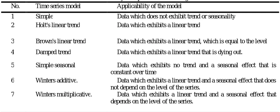
The future gap is estimated using time series forecasting techniques. The various exponential smoothing time series models (Gardner, 1985) considered for forecasting the future demand-supply gap is shown in Table 1 [6]. Apart from these exponential smoothing models, the analysis also considered ARIMA models.
Table I. Summary of exponential smoothing models No. Time series model Applicability of the model
1 Simple Data which does not exhibit trend or seasonality 2 Holt's linear trend Data which exhibits a linear trend
3 Brown's linear trend Data which exhibits a linear trend, which is equal to the level
4 Damped trend Data which exhibits a linear trend that is dying out.
5 Simple seasonal Data which exhibits no trend and a seasonal effect that is constant over time
6 Winters additive. Data which exhibits a linear trend and a seasonal effect that does not depend on the level of the series.
7 Winters multiplicative. Data which exhibits a linear trend and a seasonal effect that depends on the level of the series.
The existing gap is calculated for the three zones and the best fit time series models are used to forecast the future gap. R squared is used as the best fit evaluation criteria. The forecast for the future gap will help to anticipate the geographic disparity and hence plan effective methodologies and procure enough resources to manage the same. The succeeding sub-section presents the details of inputs used for the gap analysis.
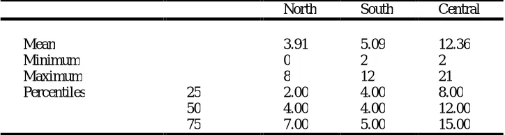
Table II. Descriptive statistics for the probable number of transplants per quarter North South Central
Mean 3.91 5.09 12.36
Minimum 0 2 2
Maximum 8 12 21
Percentiles 25 2.00 4.00 8.00 50 4.00 4.00 12.00 75 7.00 5.00 15.00
as well as interquartile range of the probable number of transplants. These values are taken equivalent to supply and gap calculations are performed as per the previously mentioned equation. These two scenarios are selected to analyse the effect of fluctuating supply on the future gap. The calculated data on present gap across the three regions is given as input to the expert modeller in IBM SPSS software. The analysis has given best fitting gap models for each of the scenarios. The detailed results are presented in the next section.
III.RESULTSANDDISCUSSION
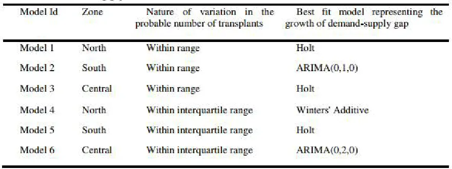
The summary of best fitting gap models obtained for various scenarios are shown in Table III. Models 1, 2 and 3 represent the forecast under the situation in which the transplants occur randomly within the range of probable transplants in the north, south and central zones respectively. The models 4, 5 and 6 represent the forecast under the situation in which the transplants occur randomly within the interquartile range of the probable transplants in the north, south and central zones respectively. The summary of forecasting results is represented in Table IV.
Table III. Best fitting gap models
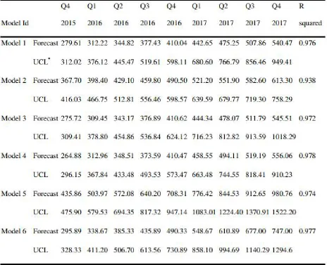
The forecasting results show that the gap is increasing for all the scenarios, with a linear trend in all the forecasting models. The predictions are made for two scenarios. The first scenario accounts for higher variability of transplants, assuming that the transplants happen within the range of probable transplants. The second scenario is based on more stable and less variable number of transplants. Assuming a higher variability in transplants, the model results predict that there will be around 1699 non-allocated patients by the end of the year 2017. The results based on interquartile range of transplants show that there will be around 2284 non- allocated patients by the end of the year 2017. Both the results show an alarming increase in the waiting list numbers. Failure to give adequate allocation priority for the medical condition of the patient could probably lead to a number of patient deaths while waiting for a kidney. The results could also manifest in the form of huge demand for live-unrelated donors which could lead to exploitation of poor donors or illegal organ trading [8].
Looking at the zone based results; south zone appears to have serious problems associated with high demand and low supply. Both the scenarios, unanimously predict that south zone will be the most adversely affected zone in near future. As per the forecasting model, first scenario with higher variance of transplants predicts an almost similar gap for the north and central zones and the second scenario predicts a higher gap for the central zone. The forecasting models predicted an almost equal or higher gap for the central zone compared to north zone because of the fact that the arrivals in central zone exhibited higher variance of arrivals along with few outliers.
Table IV. Summary of forecasting results for demand-supply gap
IV. CONCLUSION
In developing countries like India, CKD has adversely affected the society by marking a much early incidence. This creates a huge ESRD burden in countries like India, Pakistan and Bangladesh. At the same time, access to renal replacement therapy is limited to less than a quarter of the patients projected to develop ESRD in the developing regions of the world [12]. If properly implemented, the cadaver kidney transplantation program can reduce the intensity of the huge ESRD burden.
donation awareness campaigns and strengthening the public health infrastructure of adversely affected geographic zones. Also, efforts should be made to develop an allocation algorithm which can strike a balance between efficiency and equity. The gap analysis models could be improved by adding more predictors, which could explain the reason for such a growth.
REFERENCES
[1] "Kerala Organ Sharing Registry – Share Organs Save Lives", Knos.org.in. Available: http://knos.org.in/default.aspx. [Accessed: 04- Jan- 2016].
[2] H. Meier-Kriesche, F. Port, A. Ojo, S. Rudich, J. Hanson, D. Cibrik, A. Leichtman and B. Kaplan, "Effect of waiting time on renal transplant outcome", Kidney International, vol. 58, no. 3, pp. 1311-1317, 2000.
[3] A. Mathur, V. Ashby, R. Sands and R. Wolfe, "Geographic Variation in End-Stage Renal Disease Incidence and Access to Deceased Donor Kidney Transplantation", American Journal of Transplantation, vol. 10, no. 42, pp. 1069-1080, 2010.
[4] Z. Kadry, E. Schaefer, T. Uemura, A. Shah, I. Schreibman and T. Riley, "Impact of geographic disparity on liver allocation for hepatocellular cancer in the United States", Journal of Hepatology, vol. 56, no. 3, pp. 618-625, 2012.
[5] D. Stanford, J. Lee, N. Chandok and V. McAlister, "A queuing model to address waiting time inconsistency in solid-organ transplantation", Operations Research for Health Care, vol. 3, no. 1, pp. 40-45, 2014.
[6] E. Gardner, "Exponential smoothing: The state of the art", Journal of Forecasting, vol. 4, no. 1, pp. 1-28, 1985.
[7] S. Guleria, S. Aggarwal, V. Bansal, M. Varma, L. Kashyap, N. Tandon, S. Mahajan, D. Bhowmik, S. Agarwal, N. Mehra and M. Misra, "The first successful simultaneous pancreas–kidney transplant in India", The National Medical Journal Of India, vol. 18, no. 1, pp. 18-19, 2005. [8] M. Mani, "None so blind as those who will not see", The National Medical Journal Of India, vol. 15, no. 5, pp. 295-296, 2002.
[9] N. Wig, P. Gupta and S. Kailash, "Awareness of Brain Death and Organ Transplantation Among Select Indian Population", JAPI, vol. 51, pp. 455-458, 2003.
[10] M. Hossain, E. Goyder, J. Rigby and M. El Nahas, "CKD and Poverty: A Growing Global Challenge", American Journal of Kidney Diseases, vol. 53, no. 1, pp. 166-174, 2009.
[11] M. Mani, "The Nephrotoxicity Of The Tsunami", The National Medical Journal Of India, Vol. 20, No. 3, Pp. 154-155, 2007.