©
DOI: 10.1534/genetics.103.019752
An Expectation-Maximization–Likelihood-Ratio Test for Handling Missing Data:
Application in Experimental Crosses
Tianhua Niu,*
,†,1Adam A. Ding,
‡Reinhold Kreutz
§and Klaus Lindpaintner**
*Division of Preventive Medicine, Department of Medicine, Brigham and Women’s Hospital, Harvard Medical School, Boston,
Massachusetts 02215,†Program for Population Genetics, Harvard School of Public Health, Boston, Massachusetts 02115,
‡Department of Mathematics, Northeastern University, Boston, Massachusetts 02115,§Department of Clinical Pharmacology,
Benjamin Franklin Medical Center, Berlin 12200, Germany and**Roche Center of
Medical Genomics, F. Hoffmann-La Roche AG, CH-4070 Basel, Switzerland
Manuscript received July 7, 2003 Accepted for publication September 2, 2004
ABSTRACT
The mapping of quantitative trait loci (QTL) is an important research question in animal and human studies. Missing data are common in such study settings, and ignoring such missing data may result in biased estimates of the genotypic effect and thus may eventually lead to errant results and incorrect inferences. In this article, we developed an expectation-maximization (EM)–likelihood-ratio test (LRT) in QTL mapping. Simulation studies based on two different types of phylogenetic models revealed that the EM-LRT, a statistical technique that uses EM-based parameter estimates in the presence of missing data, offers a greater statistical power compared with the ordinary analysis-of-variance (ANOVA)-based test, which discards incomplete data. We applied both the EM-LRT and the ANOVA-based test in a real data set collected from F2intercross studies of inbred mouse strains. It was found that the EM-LRT makes
an optimal use of the observed data and its advantages over the ANOVAF-test are more pronounced when more missing data are present. The EM-LRT method may have important implications in QTL mapping in experimental crosses.
A
NIMAL models and their corresponding genomes parameter estimation, because the sample size for the are highly useful for mapping traits that may ap- incomplete data is less than it would be if the data were ply to human diseases (KnoblauchandLindpaintner complete. In previous literature, the treatment of such 1999). Since genes are conserved throughout evolution, a missing data problem is not adequate. Two simple the identification of “evolutionary homologs” in animals methods have been most widely applied. One is simply is well appreciated in helping to find their counterparts to use the incomplete data by deleting all data records in humans. with any values missing, and it is called “listwise dele-There are two primary methods for quantitative trait tion.” A second approach is called “pairwise deletion,” locus (QTL) mapping: (a) the single-marker method and which deletes those data records if either the phenotypic (b) the interval-mapping method. The single-marker data or the genotypic data at the marker of interest method is a traditional method for detecting the asso- are missing. In this article, we propose an expectation-ciation between individual genetic markers and the quan- maximization (EM)–likelihood-ratio test (LRT) to incor-titative trait of interest (Luoet al.2000). The analysis- porate the flanking markers’ information in the presence of-variance (ANOVA) represents the typical method of missing marker data in the single-marker analysis. The applied in this kind of analysis. The interval-mapping LRT is derived from the maximum likelihood calculated method uses information provided by multiple linked using the EM algorithm based on all the observed data. markers to probabilistically assess potential QTL at In the following section, we first introduce the mathe-chromosomal locations between such markers. In the matical model and notations, and then we derive the interval-mapping approach developed byLanderand EM algorithm for maximum-likelihood estimation. Af-Botstein(1989), evidence for a putative QTL is sum- terward, we describe the EM-LRT (or the EM-based Stu-marized by a LOD (log of odds) score that exceeds a dent’st-test) and the standard ANOVA-based tests (F-test predefined threshold at a given chromosomal position. and pairwiset-test). Then, we assess the validity of the EM-The presence of missing data in studies usually lowers
LRT at various sample sizes and various proportions of both the power of QTL mapping and the precision of
missing data, compare the performances of the proposed EM-based tests over the ANOVA-based tests through simu-lations, and evaluate whether or not it represents a more 1Corresponding author:Division of Preventive Medicine, Department
effective test for real data sets. Finally, we provide a
summa-of Medicine, Brigham and Women’s Hospital, 900 Commonwealth
Ave., Boston, MA 02215. E-mail: [email protected] rization and some further discussions.
We have implemented the algorithm described in this L()⫽
兺
ni⫽1
li(), (2)
article in the freely available statistical software R (Ihaka
andGentleman1996). The code is available from the whereli() is defined as follows. First, if the phenotypeYiand
the three genetic markersX1,i,X2,i,X3,iare all observed for the
authors upon request.
ith animal, obviously,
li()⫽l(Yi,X1,i,X2,i,X3,i,); (3)
MATERIALS AND METHODS
second, if the phenotypeYi is observed but some genetic markers
Model settings and notations:Let us denote the genotypes are missing for theith animal, then
at the trait marker locus A (the hypothesized QTL for the trait) asAA,Aa, andaa, the genotypes at its left-side flanking
marker locus B asBB, Bb, bb, and the genotypes at its right- li()⫽log ⎛ ⎜ ⎝j僆
兺
X1,i兺
k僆X2,i
兺
l僆X3,i
pj,k,l
√2exp
冦
⫺(Yi⫺ j)2
22
冧
⎞ ⎟ ⎠
; (4) side flanking marker locus C asCC,Cc, andcc(note that we
consider here only the biallelic markers, such as the simple
and third, if the phenotypeYi is missing for theith animal,
sequence length polymorphisms). LetYdenote the phenotype value; letX1,X2, andX3denote the respective genotype values
at the loci A, B, and C, whereX1⫽ 1, 2, and 3 denotes the li()⫽log⎛⎜
⎝j僆
兺
X1,i兺
k僆X2,i
兺
l僆X3,i
pj,k,l ⎞ ⎟ ⎠ . (5) three respective genotypes,AA,Aa, andaa,X2⫽1, 2, and 3
denotes the three respective genotypes,BB, Bb, andbb, and
Here and in the following, the notation of summation
兺
j僆X1,iX3⫽1, 2, and 3 denotes the three respective genotypes,CC,
Cc, andcc. LetidenoteE(Y|X1⫽i), wherei⫽1, 2, and 3. denotes the summation over all possible values of X1,i. For
example, ifX1,iis observed to be 2, then the summation
con-Then, what we test here is
tains only one case (i.e.,j ⫽2); on the other hand, ifX1,iis
H0:1⫽ 2⫽ 3(locus A isnota QTL forY), missing, then the summation is taken over all three possible
valuesj⫽1, 2, and 3.
vs.
We propose estimating the parameters by maximizing the log-likelihood L() as defined in Equations 2–5 above and Ha:1,2, and3are not all equal (locus A is a QTL forY).
using the corresponding LRT in hypothesis tests.
This hypothesis test includes the test for both dominant and Direct maximization ofL() is difficult, as we can see in additive effects of the hypothesized QTL—locus A. the complicated equations [(2)–(5)] shown above. The EM In practice, the genotype measure X1 at locus A may be algorithm (Dempsteret al.1977;LittleandRubin1987) is missing for some animals. The usual approaches for missing an appropriate method for computing the maximum-likeli-data such as listwise deletion and pairwise deletion would hood estimatorˆ when missing data are present. In the follow-simply exclude such animals from the ANOVA-based tests,
ing, we first derive formulas for the EM algorithm to maximize resulting in a lower power to detect the QTL. Here, we propose
the log-likelihoodL(). Then, we deduce the LRT using the an EM-based approach utilizing information of incomplete
EM estimations and compare its performance with the ordi-data, rather than discarding it. When there are missing data
nary ANOVA-based tests. at locus A, the approach makes use of genotype data not only
EM algorithm:We now derive the formulas of the EM
algo-at locus A, but also algo-at its two most closely linked markers, loci
rithm for this problem following standard notations ( McLach-B and C. For the three linked markers, A, McLach-B, and C, there are
lanandKrishnan1997). a total of 27 possible genotype combinations {X1⫽j,X2⫽k,
We start with an initial estimate(0) (which can be either X3⫽l}, wherej, k, l⫽1, 2, or 3. We denote the probabilities
the ANOVA estimate or any other reasonable estimate). At for the occurrence of each combination aspj,k,l⫽Pr(X1⫽j,
the (m⫹1)th iteration, we update the current estimate(m) X2⫽k,X3⫽l).
by completing the E-step and the M-step as follows. By assuming a standard ANOVA model relating the
pheno-E-step: Compute Q(,(m))⫽E[Lc()|(m), observed data].
typeYto the genotypeX1, we have
The computation is simplified to
Y⫽ X1⫹ε, (1)
Q(,(m))⫽
兺
ni⫽1
兺
3j⫽1
兺
3k⫽1
兺
3l⫽1
␦(m⫹1)
i,jkl li(), (6)
whereεⵑN(0,2) andX1can take one of the three possible
genotype values of 1, 2, or 3 defined above. The complete
where␦(m⫹1)
i,jkl ⫽ ␦i,jkl((m)) denotes the Pr(X1,i⫽j,X2,i⫽k,X3,i⫽
data set in this case is {(Yi,X1,i,X2,i,X3,i),i⫽1, . . . ,n} for a
l|observed data and (m)). It can be computed according to
sample size ofn.
The log-likelihood of the complete data is Lc()⫽ the following formula: IfYiis observed,
兺n
i⫽1l(Yi,X1,i,X2,i,X3,i,), where
␦(m⫹1) i,jkl ⫽
p(m)
j,k,lexp{⫺(Yi⫺ j(m))2/22}
兺
j僆X1,i兺
k僆X2,i兺
l僆X3,ip(m)
j,k,lexp{⫺(Yi⫺ (jm))2/22} l(Yi,X1,i,X2,i,X3,i,)⫽log
冢
pX1,i,X2,i,X3,i √2 exp
冦
⫺(Yi⫺ X1,i)
2
22
冧冣
⫻φ{j僆X1,i,k僆X2,i,l僆X3,i}; (7)
ifYiis missing, ⫽log(pX1,i,X2,i,X3,i)⫺
(Yi⫺ X1,i)
2
22
␦(m⫹1) i,jkl ⫽
p(m) j,k,l
兺
j僆X1,i兺
k僆X2,i兺
l僆X3,ip(m) j,k,l
φ{j僆X1,i,k僆X2,i,l僆X3,i}. ⫺log(√2)
(8) and ⫽(1,2,3,2, p1,1,1, p1,1,2, p1,1,3, p1,2,1, p1,2,2, p1,2,3, p1,3,1,
p1,3,2,p1,3,3, p2,1,1,p2,1,2,p2,1,3,p2,2,1, p2,2,2, p2,2,3,p2,3,1,p2,3,2, p2,3,3,p3,1,1,
Hereφ{j 僆X1,i, k 僆X2,i, l 僆X3,i} is the indicator function p3,1,2,p3,1,3,p3,2,1,p3,2,2,p3,2,3,p3,3,1,p3,3,2,p3,3,3).
whether (j,k,l) is a possible value for (X1,i,X2,i,X3,i).
M-step: Update the parameter estimate to the value ⫽
The ANOVA can also use the pairwiset-tests to examine
(m⫹1)that maximizesQ(,(m)). The maximization over
be-the phenotypic difference between two particular genotypes. comes rather simple if we further write out the expression
This pairwiset-test is used to evaluate H0:j⫽ mvs. Ha:j⬆ m for pairs of genotypesjandm(e.g., j⫽1 andm⫽2, or Q(,(m))⫽
兺
n
i⫽1
兺
3j⫽1
兺
3k⫽1
兺
3l⫽1
␦(m⫹1) i,jkl log(pj,k,l)
j ⫽ 1 and m ⫽ 3, or j ⫽ 2 and m⫽ 3). The T-statistic is calculated as
⫺
兺
i僆obs(Y)
兺
3j⫽1
兺
3k⫽1
兺
3l⫽1
␦(m⫹1) i,jkl
(Yi⫺ j)2
22
T⫽ |ˆj⫺ ˆm|
ˆ
冪
1/兺
n*i⫽1φ{X1,i⫽j}⫹1/
兺
ni⫽*1φ{X1,i⫽m}. (13)
⫺nobs(Y)log(√2).
Here, obs(Y) denotes the set ofi’s whereYiis observed, and
nobs(Y)⫽|obs(Y)|. Thet-test would reject H0 (therefore declare a phenotypic
The maximization of the above expression is very similar difference between genotypes j and m) when T ⬎ t␣/2;n*⫺3, to a linear model and we find explicitly the following updating wheret␣/2;n*⫺3is the (1⫺ ␣/2)100th percentile of at
-distribu-formula: tion with d.f.⫽(n*⫺3).
As pointed out above, the power of the ordinary ANOVA
p(m⫹1) j,k,l ⫽
兺
n
i⫽1
␦(m⫹1)
i,jkl /n, j⫽1, 2, 3, is not optimal because it does not use information for those
data records with either phenotype or genotype marker data missing. In the previous section, we proposed using the EM
k⫽1, 2, 3,l⫽1, 2, 3.
algorithm to incorporate information from the flanking loci (9)
(i.e., B and C) in the parameter estimation. Here we describe how to use these EM-based parameter estimates to develop a
(m⫹1)
j ⫽
兺i僆obs(Y)Yi(兺3k⫽1兺3l⫽1␦(i,jklm⫹1))
兺i僆obs(Y)兺3k⫽1兺3l⫽1␦(i,jklm⫹1)
, j⫽1, 2, 3. (10) statistical test that replaces the correspondingF-test (or the pairwiset-test when applicable) in the ordinary ANOVA.
Basically, theF-test in the ordinary ANOVA is replaced by
(m⫹1)⫽
冪
兺i僆obs(Y)兺3j⫽1(Yi⫺ j(m⫹1))2(兺3k⫽1兺3l⫽1␦(i,jklm⫹1))兺i僆obs(Y)兺3j⫽1兺k3⫽1兺3l⫽1␦(i,jklm⫹1)
. (11) the LRT in the EM approach as follows: (a) use the EM algo-rithm of (6)–(11) to find the parameter estimateˆ, and then compute the log-likelihoodL(ˆ) according to (1); (b) fit the The E-step and M-step are then iterated until the estimate
parameters again under H0(by the EM algorithm with
formu-(m)converges to an estimated value,ˆ.
las described in the next paragraph) to yield an estimateˆ0,
Hypothesis testing:To check whether locus A is a QTL for
and compute the log-likelihoodL(ˆ0); and (c) compute the the trait of interest,Y, statistically we test the hypothesis
likelihood-ratio statistic (LRS), H0:1⫽ 2⫽ 3(locus A isnota QTL forY)
LRS⫽2[L(ˆ)⫺L(ˆ0)]. (14) vs.
The LRT will reject H0if LRS⬎ 2␣, where2␣is the (1⫺ ␣)100th
Ha:1,2, and3are not all equal (locus A is a QTL forY). percentile of the2-distribution with d.f.⫽1.
The calculation of the LRS according to Equation 14 re-Here we first describe the ordinary ANOVA for single-marker
quires the calculations of both the maximum log-likelihood analysis, which is the standard approach in the present
litera-L(ˆ) under Haand the maximum log-likelihoodL(ˆ0) under
ture (Rubattuet al.1996;Vallejoet al.1998;Poyan Mehr
H0. We have provided in the previous section EM formulas
et al.2003; Zhaoand Meng2003). When missing data are
for fittingˆ in Equations 7–11. Here we describe EM formulas present, the ordinary ANOVA excludes all the data records
for fitting the parameters ˆ0 under H0. The EM algorithm
with missing information onX1orY, and a subset of
observa-tions is left {(Yi,X1,i),i⫽1, . . . ,n*}, (n*ⱕn). The ordinary under H0is simpler because1⫽ 2⫽ 3⫽ . Therefore,
ANOVA then estimates the mean phenotype given the geno- we would estimateby the overall sample mean under H0.
type data, Correspondingly, the variance is estimated by the sample vari-ance. That is, we can get the estimates without going through
ˆj⫽
兺
n*i⫽1
Yiφ{X1,i⫽j}, j⫽1, 2, 3, any iterations:
ˆj⫽ ˆ ⫽Y⫽
1
n*
兺
n*
i⫽1
Yi, j⫽1, 2, 3 (10⬘)
whereφis an indicator function. The variance is estimated by
ˆ2⫽ 1
n*⫺3
兺
n*
i⫽1
(Yi⫺ ˆX1,i)
2.
ˆ ⫽
冪
1n*
兺
n*
i⫽1
(Yi⫺Y)2. (11⬘)
Then, anF-test is constructed by comparingˆ2with the
be-tween-group variance,ˆ2
b, Thus, for estimatingpj,k,l’s, we need to iterate only between
the E-step,
ˆ2
b⫽
1 3⫺1
兺
n*
i⫽1
(ˆX1,i⫺Y)
2,
␦(m⫹1) i,jkl ⫽
p(m) j,k,l
兺j僆X1,i兺k僆X2,i兺l僆X3,ip
(m) j,k,l
φ{j僆X1,i,k僆X2,i,l僆X3,i} ,
whereY⫽(1/n*)
兺
in⫽*1Yi. Therefore, theF-test statistic is con- (8⬘)structed as
and the M-step,
F⫽ ˆ 2 b
ˆ2. (12)
p(m⫹1) j,k,l ⫽
兺
n
i⫽1
␦(m⫹1)
i,jkl /n, j⫽1, 2, 3,k⫽1, 2, 3,l⫽1, 2, 3.
TheF-test would reject H0ifF⬎F␣;2,n*⫺3, whereF␣;2,n*⫺3is the (9⬘)
(1⫺ ␣)100th percentile of anF-distribution with d.f.⫽2 and
RESULTS that are the values of (9⬘) at convergence. Thenˆ0is plugged
into Equation 1 to calculate L(ˆ0), which is then used to
Assessment of the validity of EM-LRT in finite
sam-compute the LRS in (14).
ples: EM-LRT is a valid test asymptotically; however, The pairwiset-test in the ordinary ANOVA is replaced by
its validity for finite sample sizes needs to be carefully a corresponding adjusted t-test in the EM approach. Since
ˆj⫺ˆm⫽兺i僆obs(Y)Yi兺k,l(␦i,jkl/兺i僆obs(Y)兺k,l␦i,jkl⫺␦i,mkl/兺i僆obs(Y)兺k,l␦i,mkl), checked. We used extensive simulations to assess the
the variance ofˆj ⫺ ˆmis approximately兺i僆obs(Y)[兺k,l(␦i,jkl/ validity of the EM-LRT for various sample sizes under
兺i僆obs(Y)兺k,l␦i,jkl ⫺ ␦i,mkl/兺i僆obs(Y)兺k,l␦i,mkl)]2ˆ2. The adjustedt-test various proportions of missing data.
statistic,T, for testing the pair of genotypesjandmis
We simulated a data set ofnanimals with the pheno-type measurement (Yi) and three genetic markers (X1,i,
T⫽ |ˆj⫺ ˆm|
ˆ
冪
兺
i僆obs(Y)关兺
k,l(␦i,jkl/兺
i僆obs(Y)兺
k,l␦i,jkl⫺ ␦i,mkl/兺
i僆obs(Y)兺
k,l␦i,mkl)兴2
,
X2,i,X3,i) for each animali: {(Yi,X1,i, X2,i,X3,i)}, where
i ⫽ 1, . . . , n. The phenotype Y for each animal was (15)
generated according to the linear model: Equation 1, whereˆj,ˆm, andˆ are from the EM estimate,ˆ. Thet-test would
with parameters 1⫽ 2⫽ 3⫽ 100 and ⫽10. We
reject H0whenT ⬎t␣/2;n⫺30, wheret␣/2;n⫺30is the (1⫺ ␣/2)100th
assigned pj,k,l to be proportional to (4 ⫺ j) ⫹ (4 ⫺
percentile of at-distribution with d.f.⫽(n⫺30).
k) ⫹ (4 ⫺ l). [We initially intended to simulate pj,k,l
As the proportion of missing data increases, but is kept
below the upper limit such that the type I error is not inflated, proportional toj⫹k⫹l. However, asj⫽1 denotes the we would expect the EM-LRT to perform better than the homozygous wild-type genotype, it should have higher ANOVA-based test in the single-marker analysis. probability than
j⫽3. Hence, we used the
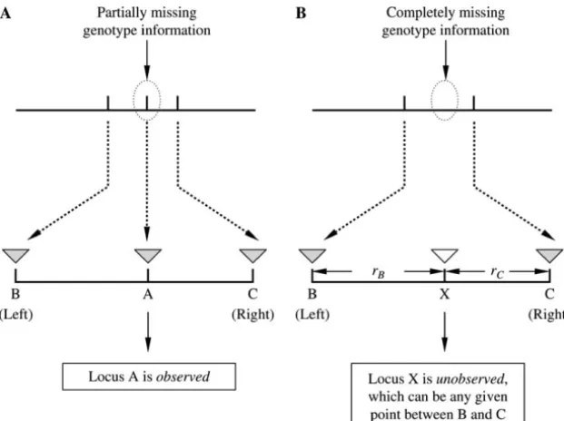
transforma-Comparison with the interval-mapping method:The
pro-tions (4⫺j) to flip the probabilities.] We then randomly posed EM-LRT above uses the genotype information at
flank-dropped phenotype observations at the trait marker ing marker loci to allow more efficient QTL detection at the
trait locus when there are missing genotype or phenotype data. locus A according to a missing probability.
The idea of using genotype information at flanking marker For each data set, we first fitted the EM estimates ˆ loci for capturing information of incomplete data is similar
through iterations of Equations 6–11. The iteration to the idea adopted by the interval-mapping method (Lander
started with the initial estimates: andBotstein1989). The interval-mapping method also uses
the EM algorithm to incorporate flanking markers’ genotype
(0)
j ⫽Y, j⫽ 1, 2, 3;
information for inferring the association (expressed as a LOD score) of the phenotypic trait with genetic variation at any
given point between the two flanking markers, but there is a (0) ⫽
冪
1n*
兺
n*
i⫽1
(Yi⫺Y)2,
significant difference between our method and the interval-mapping method. First, the main strategy is different. Our
method is exactly a single-marker test when no data are miss- p(0)
j,k,l ⫽1/27, j⫽ 1, 2, 3,k⫽1, 2, 3,l⫽1, 2, 3.
ing, and it uses information of the flanking markers only when
data are missing at the marker of interest; in contrast, the The iteration would stop when a convergence criterion interval-mapping method intends to “screen” any given point,
of 10⫺4relative change was met. Next, we fitted the EM
locusX, in the interval bracketed by two linked markers,
assum-estimatesˆ0again under H0through Equations 8⬘–11⬘.
ing (a) genotypic variation at such theoretical point exists and
(b) its recombination rates from the two flanking markers are Thenˆ andˆ0were used in computing the LRS in (14).
correctly specified. Therefore, the trait locusXis a putative We repeatedly ran the simulation 1000 times. For locus and is totally unobserved, and the interval-mapping
each simulated data set, we computed the EM-LRT (14) method uses recombination rates,rBandrC, to compute the
and recorded their values. The empirical type I error conditional probabilitiespj
k,l⫽Pr(X1⫽j|X2⫽k,X3⫽l), thus
reducing the number of parameters to 2. However, such reduc- of EM-LRT was calculated as the proportions of the tion of the number of parameters is valid only if the underlying 1000 data sets where H
0was rejected at the significance
assumptions regarding the recombination rates (i.e., rBand
level␣ ⫽0.05.
rCin Figure 1) hold. Our proposed EM-LRT, on the other
We simulated for n ⫽ 50, 100, 200, 500, and 1000, hand, makes no assumptions on the recombination rates (i.e.,
rBandrC), but instead it computespj
k,lthroughpj,k,l⫽Pr(X1⫽ respectively. For each sample size ofn, we increased the j,X2⫽k,X3⫽l), only if there are some incomplete phenotype missing probability from 10% upward, until the type I
data or genotype data at locus A (Figure 1). For convenience error exceeds the nominal significance level␣ ⫽0.05 of mathematical derivation, we have written our formula in
significantly (that is, it exceeds by two standard devia-terms ofpj,k,l. Hence our EM-LRT involves 27pj,k,l’s and we did
not reduce them to two parameters,rBandrC, which are used tions, 2
√
0.05⫻0.95/1000 ⫽0.014). Table 1 shows the in interval-mapping methods. However, the trade-off is that type I error for EM-LRT for various sample sizes. our EM-LRT is more generic with no model assumptions on As shown in Table 1, for a small sample size (n⫽50), the specification of recombination rates: for example, for verythe EM-LRT is valid for up to 10% missing observations. tightly linked markers, it has been shown that the rate of
Whenn ⫽100, the EM-LRT is valid when as much as recombination is no longer a monotone function of the
physi-cal distance (Thompsonet al.1988), and the assumption of the 20% data were missing. When n ⫽ 200, the EM-LRT interval-mapping method would appear to be overly strong. can tolerate up to 50% missing data. These simulations Under such circumstances, when there are missing data, our
showed that we have to be careful in applying the EM-LRT is still valid. We therefore consider our EM-LRT as
EM-LRT. For a small sample (e.g., n ⫽ 40), which is
acomplimentarymethod for the interval-mapping method,
Figure1.—A schematic illustrating (a) EM-LRT and (b) the interval-mapping method. The shaded inverted triangles indicate ob-served markers, the open inverted triangle in-dicates the putative locus.
error rates were 0.060 and 0.077 for 10 and 20% missing, (i.e.,j’s and2) were not much affected by the
accura-cies of the estimates ofpj,k,l’s. All parameters were
esti-respectively. Thus, forn⫽40 (see the real example in
III shown below), we can still use EM-LRT if 10% or mated more accurately when the sample sizenbecame larger. As a result, the EM-LRT is a valid test for increas-fewer observations are missing. When there areⱖ200
animals, we can use the tests with up to half of all obser- ingly greater missing proportions asn becomes larger. Power comparison of EM-LRT with ANOVA-based vations missing.
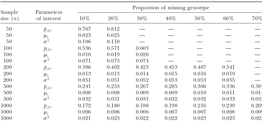
To evaluate the accuracy of parameter estimates, we tests: To compare the power of EM-LRT with that of the ANOVA-based test, we conducted simulation studies calculated the coefficient of variability (CV) for each
model parameter estimate. CV is conventionally defined using two types of phylogenetic models.
Simulation models: In the simulations performed, ge-as
√
MSE(ˆ)/, where MSE(ˆ) denotes the mean squarednetic markers were generated according to two phyloge-error of the estimate for parameterover 1000
simula-netic models (Figure 2). Let A, B, and C denote the tion runs. Table 2 shows the average CV for estimates
wild-type alleles anda,b,ctheir corresponding mutant ofpj,k,l’s,j’s, and2. (It turned out the CVs for estimates
alleles for the three loci,A,B, andC, respectively. We ofpj,k,l’s were rather similar and thus we presented only
assume that theA→ a event has arisen before either their average values.)
B→b or C→ coccurred, andB →b or C→ cevents It can be seen that the ancillary parameterspj,k,lwere
occurred only on theaBChaplotype. In model I, the estimated less accurately compared to the estimates of
B→ btook place first on the ancestral haplotypeaBC, the main parametersjand2across the board.
How-followed by the mutation of locusC on the haplotype ever, becausepj,k,l’s are parameters that are used only in
abC, resulting in four distinctive haplotypes:ABC,aBC, the adjustment of the impacts of the missing data on
the main parameters, the main parameters of interest abC, andabc. In model II, the mutation at locusBtook
TABLE 1
The empirical type I error of EM-LRT over 1000 simulations
Proportion of missing genotype
Sample size (n) 10% 20% 30% 40% 50% 60% 70%
50 0.059 0.068 — — — — —
100 0.043 0.055 0.072 — — — —
200 0.046 0.055 0.061 0.060 0.060 0.086 —
500 0.054 0.055 0.049 0.048 0.052 0.058 0.088
1000 0.060 0.048 0.056 0.051 0.048 0.046 0.081
TABLE 2
The average CVs for the parameter estimates of EM-LRT over 1000 simulations
Proportion of missing genotype Sample Parameters
size (n) of interest 10% 20% 30% 40% 50% 60% 70%
50 pj,k,l 0.767 0.812 — — — — —
50 j 0.023 0.025 — — — — —
50 2 0.106 0.110 — — — — —
100 pj,k,l 0.536 0.571 0.603 — — — —
100 j 0.018 0.019 0.020 — — — —
100 2 0.071 0.073 0.074 — — — —
200 pj,k,l 0.386 0.402 0.423 0.453 0.487 0.541 —
200 j 0.013 0.013 0.014 0.015 0.016 0.019 —
200 2 0.051 0.051 0.052 0.053 0.053 0.055 —
500 pj,k,l 0.241 0.253 0.267 0.285 0.306 0.336 0.387
500 j 0.008 0.008 0.009 0.009 0.010 0.011 0.014
500 2 0.032 0.031 0.031 0.032 0.032 0.033 0.033
1000 pj,k,l 0.172 0.180 0.188 0.198 0.216 0.239 0.269
1000 j 0.006 0.006 0.006 0.007 0.007 0.008 0.009
1000 2 0.021 0.023 0.022 0.022 0.023 0.023 0.023
Note that the average CVs for the parameter estimates were calculated only at those proportions of missing data when the EM-LRT remains valid or when the type I error starts to be inflated.
place first on the ancestral haplotypeaBC, followed by lociA,B, andC, respectively (e.g., genotype “aaBbCC” the mutation of locusCon the haplotypes bearing either corresponds toX1⫽3,X2⫽2,X3⫽1);
the wild-type allele (i.e.,aBC) or the mutant allele (i.e.,
model IB: the genotype measures X1,X2, andX3 refer
abC) at locusB, resulting in five distinctive haplotypes:
to lociB,A, andC, respectively (e.g., genotypeaaBbCC ABC,aBC,abC,aBc, andabc.
now corresponds toX1⫽ 2,X2 ⫽3,X3⫽1).
In model I, we assume thatC →c occurredonly on theabChaplotype, as shown in Figure 2. Letpadenote
In model II, we considered the case whereB →b and the proportion of the “a” allele in the population, pb
C →cevents were independent (see Figure 2); without denote the probability of theB→ b event conditional
loss of generality, we assume thatB →boccurred before on the A → a event, and pc denote the probability of
C →c. Under this model,paandpbwere defined similarly
the C→ cevent conditional on the B→ bevent. Two
as we defined in model I, butpcis defined as the
probabil-variants of model I were considered:
ity of theC→cevent conditional on the A →aevent. In our simulations, we considered the following pa-model IA: the genotype measuresX1,X2, andX3refer to
Figure 3.—Power estimation and comparison of the EM-LRT and ANOVAF-test when P(A → a)⫽20%. The points plotted indi-cate the empirical proportion of tests (by use of a nominal level␣ ⫽ 0.05) that rejected the H0among
1000 simulated data sets.K⫽ ⌬/ (/√n). Plots on the left corre-spond to cases with 10% missing data. Plots on the right corre-spond to cases with 20% missing data. * indicates cases whereP⬍
0.05, and ** indicates cases where
P⬍0.005. Here “P” refers to the
P-value of Wilcoxon rank-sum tests comparing the power differ-ence between the EM-LRT and theF-test. Solid diamonds denote the power of the EM-LRT; solid squares denote the power of the ANOVAF-test.
rameter settings forpa,pb, andpc:pb⫽pc⫽0.8, andpa various values of⌬and for different missing
probabili-ties (10 and 20% on the left-hand and right-hand sides, of values 0.1, 0.2, and 0.4. For example,pa⫽0.2 would
mean that theaallele is present in 20% of the popula- respectively for Figures 3–5). The simulated ⌬ values tion, and henceⵑ32% of the animals have the genotype were defined asK/
√
n, whereK⫽0, 1, 2, . . . . For the Aaand 4% have the genotype aa. simulation runs withpa ⫽ 0.1 (Figure 5), we replacedSimulation and fitting procedures:For these models, we the comparison between EM-LRT (14) and ANOVAF-test simulated forn ⫽ 200: {(Yi, X1,i,X2,i,X3,i)}, wherei⫽ (12) with the comparison between the EM-adjusted
1, . . . , n. The phenotype Y for each animal is again t-test (15) and the ANOVAt-test (13) for the following generated according to the linear model—Equation 1, reason: when the minor allele (a) frequency is low (pa⫽
with parameters1⫽ 100⫺ ⌬,2 ⫽100,3 ⫽100⫹ 0.1), it would be expected that only ⵑ1% of animals ⌬, and ⫽10. Here we randomly dropped values from would carry theaagenotype. Since a total of 200 animals each variable with a probability,pm. We conducted simu- were in each simulation, there were on average⬍2
ani-lations under two scenarios: (a)pm⫽10% and (b)pm⫽ mals with theaagenotype in most simulated data sets.
20%. Note that in our simulations used for assessing In many simulation runs, there was not a single observa-the validity of EM-LRT in finite samples, observa-the missing tion in theaagenotype group. Therefore, in this case, proportion refers to the missing probability ofX1. Here, the phenotypic comparison is needed only between the
pmrefers to the missing probability of all variables,Y,X1, pair of genotypesAAandAa, with respective mean
val-X2, andX3. The validity of the EM-LRT for the simulation ues denoted as1and2. It was thus more appropriate
used here was verified by checking the values of the to compare the power of the EM-adjusted t-test (15) empirical type I error rates (i.e., when⌬ ⫽ 0). with that of the ordinary ANOVAt-test (13).
For each model setting, we repeatedly ran the simula- Power comparisons:For a hypothesis test, a type I error tion 1000 times. For each simulated data set, we com- occurs if H0 is rejected when it is true. If H0 holds, a
puted the EM-LRT (14) and ANOVAF-test (12) statistics correct test should have a type I error rateⱕ ␣. The H0
and recorded their values. The empirical powers of the in this case was represented by⌬ ⫽0 (or equivalently, EM-LRT andF-test were calculated as the proportions K⫽ 0) or the left-most case in Figures 3–5. It can be of data sets where H0 was rejected at the significance seen that in those cases the empirical type I error rates
level␣ ⫽ 0.05. Figures 3 and 4 display the empirical for both the EM-LRT and the ANOVAF-test were close powers from the 1000 simulation runs forpa⫽0.2 and to␣ ⫽0.05, confirming that they were both valid tests.
Figure 4.—Power estimation and comparison of the EM-LRT and ANOVA F-test whenP(A→ a)⫽40%. The points plotted indi-cate the empirical proportion of tests (by use of a nominal level␣ ⫽ 0.05) that rejected the H0among
1000 simulated data sets.K⫽ ⌬/ (/√n). Plots on the left corre-spond to cases with 10% missing data. Plots on the right corre-spond to cases with 20% missing data. * indicates those cases where
P⬍ 0.05, and ** indicates those cases whereP⬍0.005. Here “P” refers to theP-value of Wilcoxon rank-sum tests comparing the power difference between the EM-LRT and the F-test. Solid dia-monds denote the power of the EM-LRT; solid squares denote the power of the ANOVAF-test.
it is clear that a test with a higher power is preferred. and a strain with high brain weight (BXD5). Brain vol-ume, striatal volvol-ume, striatal neuron number, striatal neu-It can be seen from Figures 3 and 4 that the empirical
powers of EM-LRT were higher than the empirical pow- ron number residual, striatal volume residual, and brain weight were measured using standard procedures. We ers of theF-test. Due to simulation variations, however,
a higher empirical power does not necessarily mean the studied a total of 13 microsatellite markers—9 markers on chromosome 10 (D10Mit106,D10Mit3,D10Mit194, real power is higher. To see whether the difference in
power is statistically significant, we conducted a pairwise D10Mit61,D10Mit186,D10Mit266,D10Mit233, D10Mit-179, andD10Mit180), and 4 markers on chromosome 18 nonparametric test (the Wilcoxon rank-sum test) on the
1000 pairs of P-values for EM-LRTs and F-tests. The (D18Mit20,D18Mit120,D18Mit122, andD18Mit184). The map locations of the loci studied were obtained from cases where the powers of EM-LRTs are statistically
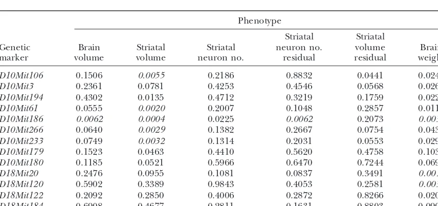
sig-nificantly higher are indicated by asterisks in the figures. Ensembl (http://www.ensembl.org/Mus_musculus/). TheP-values of both the ANOVAF-test and EM-LRT As illustrated in Figures 3 and 4, whenpm⫽10%, the
power of the EM-LRT was significantly higher than that are displayed in Tables 2 and 3.
Since few missing observations were present in the data, of F-test when K ⬎ 3 for models IA, IB, and II. And
whenpm⫽20%, the EM-LRT started to outperform the the differences inP-values were very small between the
ANOVA F-tests (Table 3) and the EM-LRT (Table 4). F-test whenK⫽2. Not surprisingly, the power
improve-ment of EM-LRT over theF-tests became more signifi- Both methods showed thatD10Mit186affects most phe-notypes in the study. Also, two markers on chromosome cant when more data were missing.
The comparison results shown in Figure 5 were simi- 18,D18Mit20 andD18Mit120, significantly affect brain weight.
lar to those of Figures 3 and 4: when 10% of data were
missing, the EM-adjusted t-test started to significantly To illustrate the effects of missing genotype observa-tions, we randomly dropped 10% of the genotype obser-outperform the ordinary ANOVAt-test forK⫽3 or 4;
when 20% of data were missing, the better performance vations at the interested locus and recalculated the P-values of the ANOVA and EM-LRT. Table 5 presents started whenK⫽2.
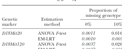
Application to a real data set in experimental crosses: the P-values of the ANOVA F-test and EM-LRT for all phenotypes of interest with and without the dropped As an illustration, we applied the proposed method to
a real data set based on an F2intercross study. This data D10Mit186 genotype data. Similarly, Table 6 presents
theP-values of the ANOVAF-test and EM-LRT for brain set, based on a previously published report (Rosenand
Williams2001), consisted of a total of 36 mice from an weight with and without the dropped D18Mit20 and D18Mit120genotype data.
Figure 5.—Power estimation and comparison of the EM-adjusted
t-test and the ordinaryt-test when
P(A→a)⫽10%. The points plot-ted indicate the empirical propor-tion of tests (by use of a nominal level␣ ⫽0.05) that rejected the H0 among 1000 simulated data
sets. K⫽ ⌬/(/n). Plots on the left correspond to cases with 10% missing data. Plots on the right correspond to cases with 20% missing data. * indicates those cases whereP⬍0.05, and ** indi-cates those cases whereP⬍0.005. Here “P” refers to theP-value of Wilcoxon rank-sum tests compar-ing the power difference between the EM-adjustedt-test and the or-dinaryt-test. Solid diamonds de-note the power of the EM-adjusted
t-test; solid squares denote the power of the ordinaryt-test.
As we can see from these tables, P-values for the detect the association under the same condition. On the other hand, as shown in Table 5, the effect of drop-ANOVAF-tests were more sensitive to the dropped
phe-notype data than were those for the EM-LRT. For exam- ping 10%D10Mit186genotype data is less pronounced. The results produced by ANOVA tests led to the same ple, in Table 6, the ANOVA tests are no longer able to
detect the association at the␣ ⫽0.01 level with brain conclusions on the associations of theD10Mit186 geno-type with all the phenogeno-types except the striatal neuron weight when 10% of genotype observations at the
inter-ested locus were dropped while the EM-LRT can still number residual. The ANOVA test was not able to detect
TABLE 3
TheP-values of the ANOVAF-test for associations between the phenotypes and genetic markers
for the mouse data
Phenotype
Striatal Striatal
Genetic Brain Striatal Striatal neuron no. volume Brain
marker volume volume neuron no. residual residual weight
D10Mit106 0.1506 0.0055 0.2186 0.8832 0.0441 0.0240
D10Mit3 0.2361 0.0781 0.4253 0.4546 0.0568 0.0261
D10Mit194 0.4302 0.0135 0.4712 0.3219 0.1759 0.0229
D10Mit61 0.0555 0.0020 0.2007 0.1048 0.2857 0.0118
D10Mit186 0.0062 0.0004 0.0225 0.0062 0.2073 0.0037
D10Mit266 0.0640 0.0029 0.1382 0.2667 0.0754 0.0438
D10Mit233 0.0749 0.0032 0.1314 0.2031 0.0553 0.0290
D10Mit179 0.1523 0.0463 0.4410 0.5620 0.4758 0.1031
D10Mit180 0.1185 0.0521 0.5966 0.6470 0.7244 0.0697
D18Mit20 0.2476 0.0955 0.1081 0.0837 0.3491 0.0012
D18Mit120 0.5902 0.3389 0.9843 0.4053 0.2581 0.0037
D18Mit122 0.2092 0.2850 0.4006 0.2872 0.8266 0.0208
D18Mit184 0.6908 0.4677 0.2811 0.1631 0.8803 0.0904
TABLE 4
TheP-values of EM-LRT for associations between the phenotypes and genetic markers for the mouse data
Phenotype
Striatal Striatal
Genetic Brain Striatal Striatal neuron no. volume Brain
marker volume volume neuron no. residual residual weight
D10Mit106 0.1268 0.0035 0.1904 0.8733 0.0332 0.0171
D10Mit3 0.2057 0.0568 0.3822 0.5158 0.077 0.0232
D10Mit194 0.3488 0.0101 0.5458 0.3501 0.2025 0.0123
D10Mit61 0.0426 0.0012 0.1735 0.0854 0.2549 0.0079
D10Mit186 0.0039 0.0002 0.0160 0.0039 0.1796 0.0022
D10Mit266 0.0391 0.0012 0.1067 0.2279 0.0492 0.0261
D10Mit233 0.0536 0.0016 0.1003 0.1952 0.0339 0.0197
D10Mit179 0.1284 0.0350 0.4093 0.5334 0.4448 0.0838
D10Mit180 0.1284 0.0350 0.4093 0.5334 0.4448 0.0838
D18Mit20 0.4458 0.1223 0.2379 0.1652 0.3077 0.0010
D18Mit120 0.5360 0.3015 0.9819 0.3581 0.1829 0.0017
D18Mit122 0.2882 0.2364 0.4726 0.3259 0.8005 0.0125
D18Mit184 0.8812 0.2694 0.4598 0.1603 0.9425 0.0281
P-values⬍0.01 are in italics.
the association between the D10Mit186 genotype and utilize information contained in incomplete data. By using both simulated and real data sets, we demon-the striatal neuron number residual when 10% of data
were missing while the EM-LRT could still detect the strated that EM-LRT utilizing incomplete data is a valid test for finite samples with moderate proportions of association. By and large, we see that the EM-LRT
im-proves the statistical power over the case when all miss- missing values and is a more powerful test compared to ordinary ANOVA-based tests that discarded all missing ing data were excluded.
data from the analysis.
Missing information on either genotype or phenotype DISCUSSION can obscure the true genetic effect (SenandChurchill
2001). To reduce the proportion of missing data, the In this article, we presented an EM-LRT using
flank-best solution is to repeat the experiment, but it can ing markers information in single-marker analysis to
be costly and time-consuming. The EM algorithm is a standard maximum-likelihood estimation method for
TABLE 5 handling missing data (Dempster et al.1977). In the
present context, the method fractionally assigns (E-step)
TheP-values of the ANOVAF-test and the EM-LRT for
the incomplete data to their theoretically possible values
associations between the phenotypes and genetic
on the basis of the current estimates of the parameters
markerD10Mit186for the mouse data with
and then revises the parameter estimates to maximize
various proportions of missing genotype data
Proportion of
missingD10Mit186 TABLE 6
genotype
TheP-values of the ANOVAF-test and the EM-LRT for
Estimation
Phenotype method 0% 10% association between brain weight and genetic
markersD18Mit20andD18Mit120for the
Brain volume ANOVAF-test 0.0062 0.0014
mouse data with various proportions
EM-LRT 0.0039 0.0032
of missing genotype data
Striatal volume ANOVAF-test 0.0003 0.0180 EM-LRT 0.0002 0.0001
Proportion of Striatal neuron no. ANOVAF-test 0.0225 0.0231
missing genotype EM-LRT 0.0159 0.0165 Genetic Estimation
Striatal neuron no. ANOVAF-test 0.0062 0.0107 marker method 0% 10%
Residual EM-LRT 0.0039 0.0039
Striatal volume ANOVAF-test 0.2072 0.3731 D18Mit20 ANOVAF-test 0.0011 0.0166
EM-LRT 0.0010 0.0030
Residual EM-LRT 0.1796 0.1664
Brain weight ANOVAF-test 0.0036 0.0004 D18Mit120 ANOVAF-test 0.0037 0.0261
EM-LRT 0.0017 0.0011
EM-LRT 0.0022 0.0014
(the M-step) the likelihood on the basis of the pseudo- selected is independent from study I. In other words, the new genetic marker is not selected because the flanking complete data. This two-step, alternating iteration
pro-cedure is repeated until convergence can be reached. markers already showed associations with the phenotype in study I. If the new genetic marker is selected because Statistical theory guarantees that the observed data
like-lihood increases to a maximum via the algorithm, and of an association observed in regard to the flanking markers in study I, then a sequential design is needed. thus the EM-LRT can be performed validly (Dempster
et al.1977). Likelihood methods with the EM algorithm How to adjust our tests for the sequential design is an interesting research topic that deserves further investi-allow the recovery of much of the lost information and
make statistically efficient use of the data. In the simu- gation.
lated data sets, the EM-LRT outperforms the ANOVA- We are grateful to the two anonymous reviewers for their comments based tests at various marker allele frequencies, and and suggestions. We thank Glenn D. Rosen at the Beth Israel Deacon-ess Medical Center, Harvard Medical School for providing the mouse
the differences in statistical power became increasingly
inbred strain data.
more pronounced with an increasing portion of missing data or an increasing value of⌬ (Figures 3–5). In the real data set example on inbred mouse strains, we found
LITERATURE CITED that with 10% missing data the significant associations
Dempster, A. P., N. M. LairdandD. B. Rubin, 1977
Maximum-of D18Mit20 and D18Mit120 with brain weight could
likelihood estimation from incomplete data via the EM algorithm.
still be detected by EM-LRT, but not by ANOVA-based J. R. Stat. Soc. Ser. B39:1–38.
tests. Taken together, we argue that the EM-LRT is an Ihaka, R., andR. Gentleman, 1996 R: a language for data analysis and graphics. J. Comp. Graph. Stat.5:299–314.
attractive statistical method that can utilize information
Knoblauch, M., andK. Lindpaintner, 1999 Use of animal models
from incomplete data. to search for candidate genes associated with essential hyperten-The EM-LRT is a valid test asymptotically (i.e., a large sion. Curr. Hypertens. Rep.1:25–30.
Lander, E. S., andD. Botstein, 1989 Mapping Mendelian factors
n). For finite samples, our simulations indicated that,
underlying quantitative traits using RFLP linkage maps. Genetics
forn⫽100, the method can tolerate up to 20% missing 121:185–199.
genotype data; forn ⫽ 200, the method can tolerate Little, R. J. A., andD. B. Rubin, 1987 Statistical Analyses With Missing Data.Wiley, New York.
up to 50% missing genotype data. Thus, there is another
Luo, Z. W., S. H. TaoandZ-B. Zeng, 2000 Inferring linkage
disequi-potential application of the proposed EM-LRT for a librium between a polymorphic marker locus and a trait locus combined analysis of different studies. For example, in natural populations. Genetics.156:457–467.
McLachlan, G. J., andT. Krishnan, 1997 The EM Algorithm and
suppose in study I (with a sample size ofn1) that we
Extensions.Wiley, New York.
already collected phenotype data and genotype data on Poyan Mehr, A., A. K. Siegel, P. Kossmehl, A. Schulz, R. Plehm D10Mit61andD10Mit266, and later we decide to study et al., 2003 Early onset albuminuria in Dahl rats is a polygenetic trait that is independent from salt loading. Physiol. Genomics
other nearby genetic markers, sayD10Mit186as well as
14:209–216.
D10Mit61andD10Mit266in a new, independent study, Rosen, G. D., andR. W. Williams, 2001 Complex trait analysis of study II (with a sample size ofn2). We might combine the mouse striatum: independent QTLs modulate volume and
neuron number. BMC Neurosci.2:5–16.
study I with study II by treating theD10Mit186genotype
Rubattu, S., M. Volpe, R. Kreutz, U. Ganten, D. Gantenet al., 1996
data as missing in study I, and then the EM-LRT can Chromosomal mapping of quantitative trait loci contributing to be used to detect the association between the phenotype stroke in a rat model of complex human disease. Nat. Genet.13:
429–434.
of interest andD10Mit186by merging studies I and II
Sen, S., andG. A. Churchill, 2001 A statistical framework for
quan-together (with a sample size ofn1⫹n2). When we use titative trait mapping. Genetics159:371–387.
this approach to combine different studies, we have to Thompson, E. A., S. Deeb, D. WalkerandA. G. Motulsky, 1988 The detection of linkage disequilibrium between closely linked
pay particular attention to the assumption of “missing
markers: RFLPs at the AI-CIII apolipoprotein genes. Am. J. Hum.
at random.” That is, the genotype missing probability Genet.42:113–124.
is not related to the phenotype value. This can be en- Vallejo, R. L., L. D. Bacon, H. C. Liu, R. L. Witter, M. A. Groenen et al., 1998 Genetic mapping of quantitative trait loci affecting
sured by checking that the animals in different studies
susceptibility to Marek’s disease virus induced tumors in F2 in-come from exactly the same genetic backgrounds (e.g., tercross chickens. Genetics148:349–360.
common F0parents) under the same experimental and Zhao, J., andJ. Meng, 2003 Genetic analysis of loci associated with partial resistance to Sclerotinia sclerotiorum in rapeseed
(Bras-breeding conditions. The tests developed in this article
sica napus L.). Theor. Appl. Genet.106:759–764.
can be applied to the combined (studies I and II