ABSTRACT
JENKINS, JONATHAN PAUL. End-to-end Noncontiguous Access Pattern Optimization for Extreme-scale Scientific Data Analytics. (Under the direction of Dr. Nagiza F. Samatova.)
In high-performance computing (HPC) environments, numerous factors conspire to make ef-ficiently accessing large-scale scientific data difficult: the continually growing imbalance between compute and I/O capabilities, the data intensive nature of current and future scientific simu-lations, the distribution of data among many discrete storage locations in parallel filesystems, and the complexity of data access patterns in I/O workloads.
Driven by these observations, two worthwhile goals to consider for the purpose of removing bottlenecks from, and otherwise optimizing, I/O in an HPC context is reducing the size of access through data reduction and reducing the complexity of mapping noncontiguous data accesses to storage through data organization policies in parallel filesystems. Techniques for the former can aid in mitigating the compute-I/O gap, while techniques for the latter can help extract the maximum performance from the underlying storage system.
In this thesis, we propose complementary approaches to reduce both the size and complexity of data accesses to parallel storage, focusing on post-data-generation analysis workloads (i.e., I/O read optimization) across the I/O software stack. Additionally, we develop methodologies to efficiently process noncontiguous data, a common occurrence in HPC data workloads, informed by current architectural trends (e.g., GPUs). For data reduction, we explore techniques of level-of-detail analysis, which aims to reduce read costs for data analysis at the cost of reduced analysis precision. While existing level-of-detail methods, such as hierarchical Z-order sampling and wavelet multiresolution analysis, have proven useful in a number of analysis tasks, they do not provide both hard bounds on data precision and full-context views of the data, both of which are essential for a robust level-of-detail methodology.
Based on these limitations, we present aprecision-basedlevel-of-detail methodology (APLOD) for scientific floating-point data, which utilizes the floating-point format to provide well-defined I/O-accuracy tradeoffs. Data layout complexity is reduced by a deterministic partitioning of data, with low computational overhead and bounded per-point errors.
The data processing required to implement APLOD induces noncontiguous access patterns, which are ubiquitous in scientific computing, commonly seen in array subvolume accesses, spatio-temporal accesses, etc. Processing these accesses, specifically for I/O, have been ex-plored at various levels of the I/O software stack. For APLOD in particular, we have shown scalable integration with the ADIOS high-level I/O library.
the MPI runtime to efficiently communicate noncontiguous data without user intervention. One significant use-case missing from such noncontiguous data processing is the ability to efficiently process data residing in graphics processing unit (GPU) memory. Hence, we develop an MPI datatypes processing algorithm optimized for GPU-resident data, utilizing the massively parallel nature of GPUs. We demonstrate low processing overhead for both regularly-structured data and irregular data, compared to methods based on PCIe direct memory access (DMA).
End-to-end Noncontiguous Access Pattern Optimization for Extreme-scale Scientific Data Analytics
by
Jonathan Paul Jenkins
A dissertation submitted to the Graduate Faculty of North Carolina State University
in partial fulfillment of the requirements for the Degree of
Doctor of Philosophy
Computer Science
Raleigh, North Carolina
2013
APPROVED BY:
Dr. Xiaosong Ma Dr. Kemafor Anyanwu
Dr. David Thuente Dr. Anatoli V. Melechko
BIOGRAPHY
ACKNOWLEDGEMENTS
There are many people that played an integral role in the completion of this dissertation, whether via direct collaboration, guidance roles, technical support or emotional support.
First and foremost, I am eternally grateful to my thesis advisor, Dr. Nagiza Samatova, for supporting me throughout the entirety of my graduate study. It goes without saying that my success as a graduate student is both a direct and indirect result of her guidance, and my future successes in the field of computer science will be a result of the personal and professional growth acheived under her tutelage. Her drive, her students-first policy, and her crystal-clear research and analytical vision is a constant source of inspiration, for which I have learned and benefitted immensely from.
I am greatly thankful of my thesis committee members: Professors Kemafor Ogan, Xiaosong Ma, Anatoli Melechko, and David Thuente, for their valuable comments and support that have been very helpful in completing and improving upon this thesis. I am further grateful to Dr. Douglas Reeves for admission and financial support upon my entry to the NC State PhD program.
Over the period of this dissertation I have had the pleasure of collaborating with several experts at various institutions in the field of computing. At Argonne National Laboratory, I have collaborated closely with Robert Ross and Dries Kimpe, as well as Robert Latham, Pavan Balaji, Tom Peterka, and James Dinan. Additionally, the completion of my study was performed while at Argonne National Laboratory, with support by the MCS division as well as LCRC. I am also thankful of Scott Klasky at Oak Ridge National Laboratory, C.S. Chang and Stephane Ethier at Princeton Plasma Physics Laboratory, and Jackie Chen and Hemanth Kolla at Sandia National Laboratory for collaboration in various components of this thesis.
I owe a debt of gratitude to Dr. Samatova’s research group, for which I had the pleasure of daily collaboration with – both the work presented in this thesis and numerous other works outside the scope of this thesis would not have been possible without their help. Sriram Lak-shminarasimhan, David Boyuka, and Eric Schendel each played integral roles in much of this thesis, and in many other projects I have been involved in. I am especially thankful to Xiaocheng Zou and Houjun Tang for the work on RADAR. Additionally, I would like to thank Kanchana Padmanabhan for collaboration on the “Practical Graph Mining with R” book. Finally, I am also grateful for collaborations with Isha Arkatkar, Zhenhuan Gong, and Terry Rogers.
I would like to thank my family for the support that was essential throughout my graduate studies: my mother Susan, father Douglas, my brothers Jeremy, Jeffery, and sister Myra. I am truly blessed to have had their support throughout my life.
TABLE OF CONTENTS
LIST OF TABLES . . . vii
LIST OF FIGURES . . . .viii
Chapter 1 Introduction . . . 1
1.1 Hypothesis . . . 2
1.2 Proposed Approaches . . . 2
1.2.1 Precision-based Level-of-detail Processing of Big Data . . . 3
1.2.2 Representing and Processing Noncontiguous Data Layouts at the Mid-dleware Level with MPI Datatypes . . . 4
1.2.3 Dynamic, Filesystem-level Data Layout Optimization . . . 6
Chapter 2 Byte-precision Level of Detail Processing for Variable Precision Analytics . . . 9
2.1 Introduction . . . 9
2.2 Background . . . 12
2.3 Methodology . . . 13
2.3.1 Component Vector Representation and Operations . . . 15
2.3.2 Partial-precision I/O . . . 17
2.4 Experimental Evaluation . . . 18
2.4.1 I/O Performance . . . 19
2.4.2 Transform Performance . . . 20
2.4.3 Partial Precision Analysis Accuracy . . . 21
2.5 Conclusion . . . 27
Chapter 3 Enabling Fast, Noncontiguous GPU Data Movement in Hybrid MPI+GPU Environments . . . 29
3.1 Introduction . . . 29
3.2 Background . . . 31
3.2.1 MPI Datatypes Specification . . . 31
3.2.2 GPU Architecture and Programming Model . . . 33
3.2.3 GPU-GPU Communication in MPI Frameworks – MVAPICH . . . 34
3.3 In-GPU Datatype Processing . . . 34
3.3.1 MPI Datatype Encoding in GPU Memory . . . 35
3.3.2 Parallel GPU Packing Kernel . . . 37
3.3.3 Packing in the Presence of Resource Contention . . . 40
3.4 Evaluation - Microbenchmarks . . . 42
3.4.1 Test Datatypes . . . 42
3.4.2 Noncontiguous Packing Performance . . . 43
3.4.3 Noncontiguous Packing Performance by Component . . . 46
3.4.4 Full Evaluation: GPU-to-GPU Communication . . . 49
3.4.5 Resource Contention Effects on Packing . . . 50
3.6 Evaluation - APLOD in GPU Memory . . . 53
3.7 Related Work . . . 54
3.8 Concluding Remarks . . . 55
Chapter 4 RADAR: Runtime Asymmetric Data Access-driven Replication . . 58
4.1 Introduction . . . 58
4.2 Background . . . 59
4.2.1 MPI-IO, ROMIO, and ADIO . . . 59
4.2.2 PVFS and EOF . . . 60
4.3 Method . . . 60
4.3.1 Overview . . . 60
4.3.2 EOF Data Management . . . 61
4.3.3 I/O Tracer and Analyzer . . . 62
4.3.4 RADAR Layout Manager . . . 63
4.3.5 Replica-aware ADIO Driver . . . 69
4.4 Experimental Evaluation . . . 72
4.4.1 Setup . . . 72
4.4.2 RADAR-specific Setup . . . 73
4.4.3 Benchmarks . . . 73
4.4.4 Decomposition Performance . . . 74
4.4.5 Model Verifications . . . 78
4.4.6 Replica Inverted List Performance . . . 82
4.4.7 Performance with APLOD . . . 82
4.5 Related Work . . . 83
4.5.1 Replication in Storage Systems . . . 83
4.5.2 I/O Middleware and User-level Replication . . . 84
4.5.3 Capturing and Detecting I/O Access Patterns . . . 84
4.6 Conclusion . . . 85
Chapter 5 Conclusion . . . 86
5.1 Future Work . . . 86
5.1.1 RADAR Future Work . . . 86
5.1.2 Storage System Future Work . . . 88
5.1.3 Advanced Data Transform Techniques in the I/O Software Stack . . . 88
LIST OF TABLES
Table 2.1 Maximum per-point percent errors on partial-precision IEEE 754 doubles,
masking the remaining bytes with the quantity 0x7F···FF. . . 12
Table 2.2 Per-point relative errors (absolute values). . . 22
Table 2.3 Pearson Correlation between full and partial-precision data. . . 23
Table 2.4 Partial-precision relative errors for mean and standard deviation. . . 23
Table 2.5 Clustering errors, measured as the misclassification rate compared to full-precision. The uvel and vvel variables from S3D are partitioned into 10 clusters. . . 24
Table 2.6 Distribution of relative errors for real, complex, and magnitude compo-nents of FFT data generated from the GTS phi data. Total number of points is 191751.Arefers to APLOD,W refers to wavelets, and the num-ber refers to the proportion of the full dataset used (as a fraction of eight). 28 Table 3.1 MPI datatypes and their fixed/variable length parameters. The “Com-mon” row contains parameters common to all datatypes in our implemen-tation. The lookaside offset is added to point to the variable type param-eters upon serialization. . . 36
Table 3.2 Transfer of face of three dimensional matrix of double-precision values to CPU, versus cudaMemcpy2D. X-Y: fully contiguous. X-Z: z sets of x contiguous doubles. Y-Z: fully non-contiguous. . . 48
Table 3.3 User workloads in contention with the pack kernel and CUDA API calls, using the vector type, in milliseconds. The Workload column shows the order in which the operations are initiated, while the Proc. column shows the time between initialization of the packing/CUDA operation and its completion. Section 3.4.5 discusses the parameters. . . 51
Table 3.4 Packing times in milliseconds for 8 MPI ranks.CPU Pack: reference pack-ing time of data resident in CPU RAM.Copy-only: GPU-to-CPU packing time using memory copies for each GPU buffer. Kernel: GPU-to-CPU packing time using the packing kernel. . . 53
Table 4.1 Performance Model System Parameters . . . 66
Table 4.2 Performance Model Variables . . . 73
LIST OF FIGURES
Figure 1.1 I/O Software/Hardware Stack . . . 6
Figure 2.1 The partitioning of a IEEE 754 double-precision value by the CV{2,1,1,4}. 14 Figure 2.2 Byte-precision level of detail partitioning, based on a generic component
vector (CV) splitting groups of significant bytes. . . 15 Figure 2.3 Partial-precision level of detail transformation using MPI datatypes, for
CV {x, y, z}. . . 16 Figure 2.4 A double-precision variable in the ADIOS XML configuration, in both
unmodified and in APLOD format. . . 17 Figure 2.5 Parallel I/O read performance (actual and relative) using ADIOS, with
and without APLOD-reorganization. ME/s - millions of elements per sec-ond. GE/s - billions of elements per secsec-ond. . . 19 Figure 2.6 Performance of transforming from original data layout to component-level
contiguous chunks, and vice versa.A- APLOD.M - MPI datatypes. Wav-1D - one-dimensional wavelet transform. . . 21 Figure 2.7 Performance of partial-precision value reconstruction. . . 21 Figure 2.8 XGC-1 100-bin histograms. . . 25 Figure 2.9 For the D4 wavelet, a,b - Mean, median errors of FFT data along each
drift wave (real component), and c - FFT errors plotted against real component value. . . 26 Figure 2.10 For varying APLOD precisions, a,b - Mean, median errors of FFT data
along each drift wave (real component), andc- FFT errors plotted against real component value. . . 27
Figure 3.1 Array slice with a width of two elements, an MPI vector datatype CS encoding it, and the slice’s subsequent packed form. . . 31 Figure 3.2 Defining and communicating a vector-of-vectors. . . 32 Figure 3.3 Communication pattern necessitating GPU packing. Reversing the arrow
directions produces the pattern necessitating GPU unpacking. . . 35 Figure 3.4 Example type tree in CPU memory, separated and serialized preorder
into GPU memory by its fixed-and-variable-length parameters. Branches in trees only appear for structtypes. . . 37 Figure 3.5 Baseline packing time for several MPI datatypes using the CUDA API,
and relative performance of packing against CUDA. . . 44 Figure 3.6 Hand coded packing kernel times and relative generalized pack performance. 44 Figure 3.7 vectorpack performance vs.cudaMemcpy2D, with varying blocklengths. . 46 Figure 3.8 Packing time, by component. “Comp” refers to traversing the type,
Figure 3.9 GPU-to-GPU ping-pong test, on thevectortype with 8, 32, and 128 byte blocks, against cudaMemcpy2D. The vectorstride is aligned to maximize CUDA performance. . . 50 Figure 3.10 Parallel Voronoi tesselation data structure for HACC. . . 52 Figure 3.11 APLOD full precision GPU-to-CPU shuffle and CPU-to-GPU
reconstruc-tion performance. . . 54
Figure 4.1 RADAR components, across the I/O software stack. The shaded figures delineate our contributions. . . 61 Figure 4.2 EOF object layout for RADAR. . . 62 Figure 4.3 Access pattern over and under provisioning based on model optimization
on balanced accesses (for np= 2) . . . 67
Figure 4.4 Allocation units in RADAR (“Object Domains,” or ODs), and replica layout in an OD. . . 70 Figure 4.5 Replica lookup using inverted index with bin extension . . . 71 Figure 4.6 Subvolume decompositions used in our evaluation (contiguous in order
Z, Y, X, time). . . 74 Figure 4.7 Subvolume-over-time-decomposition results with different process
config-urations . . . 76 Figure 4.8 Cube-decomposition results with different process configurations . . . 77 Figure 4.9 Column-decomposition results with different process configurations . . . . 78 Figure 4.10 Row-decomposition results with different process configurations . . . 79 Figure 4.11 Model results against median empirical performance (8 clients per node). 80 Figure 4.12 Model results against median empirical performance (1 clients per node). 81 Figure 4.13 Model results against median empirical performance (1 aggregator per
node). . . 81 Figure 4.14 APLOD (two bytes precision) performance with and without RADAR.
Chapter 1
Introduction
A well-known problem in the HPC community is the ever-increasing rate of data production by large-scale scientific simulations, coupled with diverging rates of growth between dedicated compute resources and shared storage resources [53]. These conditions lead to I/O becoming a limiting factor in many data-intensive applications. This is not only a simulation-time problem, where data to be written is being generated, but also a post-simulation analysis/visualization of data, made especially important by the fact that the data flow for large-scale simulation data is typically write-once, read-many.
To mitigate the performance gap, numerous avenues of research have been explored. On the one hand, architectural advancements such as the usage of SSDs and burst buffers [58] have been closely examined to continue to increase I/O system bandwidth and responsiveness. Additionally, software-based solutions and data workflows have been developed to reduce or even eliminate the need to perform I/O, via in-situ and in-transit computations which per-form analysis operations while data is in cluster memory [61, 125, 123] or by bypassing the filesystem and forwarding data directly from the simulation to dedicated analysis/visualization resources [108]. While having been shown to be effective approaches, not all analyses are able to be done at run-time for practical reasons – data cannot perpetually be in memory, and analyses such as query-driven analysis require user input across a potentially global data context.
On the other hand, a broad range of data transformation and reorganization techniques have been developed to accelerate/ease access to, reduce the footprint of, and/or augment data in storage. There are many examples, such as reducing the storage footprint via com-pression techniques (both lossy [49, 50] and lossless [85, 10]), indexing the dataset for fast future access [39, 42], focusing on performing such transformations in-situ [87, 47], or hybrid combinations of the mentioned methods [48, 30, 29].
the following two problems: 1) read-time data reduction techniques, reducing the I/O necessary to perform accurate data analysis (related but not equivalent to reducing the physical storage size of said data), and 2) generating efficient data distributions in parallel storage based on user workload characteristics. There are numerous challenges in developing such methodologies, with both usability and efficiency concerns:
1. Integration with existing I/O libraries. Data reduction that is fully “out-of-band” would render usage and adoption in applications highly difficult.
2. Transformation speeds capable ofin-situ usage. Compression libraries such as bzip2 may be too heavyweight for in-situ application on scientific datasets (as seen by Schendel et al. [85]) and may not present enough “value-added” to justify large-scale usage.
3. Non-intrusive data modification. Related to the first point, successful data transform and reorganization techniques must attempt to avoid highly disruptive changes in data format; otherwise they risk creating non-trivial interoperability concerns.
1.1
Hypothesis
Given our I/O optimization motivations and in mind of the specific challenges behind our proposed work, we derive the following hypothesis which will be tested throughout our thesis:
For maximum I/O read performance and hence minimum time-to-analysis, compute-efficient,
read-time data reduction and distribution must be considered across the entire I/O software
stack. Furthermore, techniques must be able to work in tandem to optimize I/O in two non-exclusive domains – reducing the size of data read necessary to perform efficient analysis with
guaranteed accuracy bounds, and distributing datasets in such a way that translates complex user access patterns into simple and efficient filesystem access patterns.
1.2
Proposed Approaches
1.2.1 Precision-based Level-of-detail Processing of Big Data
In the context of the growing amount of scientific simulation data, data reduction methodologies are important tools for the computational gains of current and future supercomputers to not be outweighed by the slower rate of growth by I/O subsystems. Compression, data reduction via feature selection at run-time [61, 83, 92, 123], and other methods are active areas of research; one methodology in particular that focuses on analysis-time data reduction is level-of-detail
analysis, which refers to analyzing a subset or approximation of a full context dataset. Level-of-detail analysis allows scientists to trade off data precision and accuracy for a smaller data footprint, improving I/O performance.
Problems and Challenges
For extreme-scale data and simulations, there are a number of restrictions necessitating new level-of-detail methodologies. The most important of these isbounded per-point error, to provide a guarantee of data accuracy – sampling-based analysis and wavelet multiresolution analysis (MRA) do not provide this guarantee. Furthermore, post-processing large-scale data is increas-ingly viewed as undesirable, as evidenced by the growth of in-situ, or simulation-time, data processing methodologies and frameworks, such as DataTap/DataStager [3] and PreDatA [126]. Since in-situ support is necessary, alow-overhead data transform is required. Finally, to aid in integration as well as to ensure communication and I/O efficiency, the data layout of the level-of-detail method must besufficiently simple so as tominimally disturb existing communication and I/O patterns – general lossless compression methods are ill-suited for this.
Previous methodologies do not map well to this restricted problem space. Sampling-based level-of-detail methodologies, whether statistical database sampling [16, 32, 72, 75] or spatial sampling through data layouts such as the Z-order space-filling curve [78], do not provide a full-context view of the data, and may lose small features or sharp transitions in the data. Wavelet (MRA) [23], used heavily in image-processing and included in standards such as JPEG 2000 [99], provide strong average errors, but do not provide per-datum bounds on error. More generally, data compression techniques designed specifically with scientific data in mind, such as FPC [9, 10], FPZip [57], and ISOBAR [21], change both communication patterns for collective I/O and data layout patterns to produce data chunks not aligned to disk stripe boundaries.
Approach and Results
In order to meet these requirements, we developed an analytics-drivenprecision level-of-detail (APLOD) methodology [41]. Built for floating-point data, APLOD enables configurable level-of-detail access through specification of significant byte boundaries, which we call acomponent vector (CV). Querying data at a parameterized level of precision, along with characteristics defined in the IEEE 754 floating-point format [2], allows us to give exact upper bounds on per-point data accuracy. Furthermore, the deterministic splitting of the input floating-per-point data means access patterns are not significantly modified.
Initial results, compared against wavelet multiresolution analysis (MRA) using the GNU Scientific Library (GSL) [25], were positive from both a performance and accuracy standpoint. Performance-wise, the rate of transforming to and from the APLOD format is numerous times faster than the GSL implementation (greater than 10x for larger buffers). Accuracy-wise, the strict upper bounds on APLOD error allow analysis errors for numerous simple and more com-plex operations to scale with the degree of precision, while outliers in the wavelet-reconstructed data prevent the same from occurring in some of the metrics.
Additionally, we demonstrated how to represent the APLOD-formatted data within the popular Adaptable I/O System (ADIOS) [59], which uses a simple XML configuration format to configure data layout. By splitting variables within the XML configuration, the data layout is handled by ADIOS rather than by users, provided that the data passed to ADIOS is APLOD-transformed. For a 4x reduction in data read size via precision level-of-detail, we showed I/O performance to scale at a factor of 3.5–4x.
1.2.2 Representing and Processing Noncontiguous Data Layouts at the Mid-dleware Level with MPI Datatypes
Problems and Challenges
One question that arises is a usability versus performance one. What higher-level abstractions exist that are capable of representing APLOD operations, and what effect do the use of those frameworks have on APLOD performance? For this, we have identified two data movement middlewares that are capable of performing APLOD storage and communication. The first of which, ADIOS, we already discussed in Section 1.2.1. The second is through the Message Passing Interface’s (MPI)derived datatypes [65, 81].
The usage of MPI derived datatypes allows us to implicitly perform the APLOD transform through the communication layer. Through derived datatypes, which defines a noncontiguous data space to perform communication and I/O, we showed how to map any APLOD format into an equivalent MPI datatype. However, it was shown that the representation resulted in an up-to 10x performance regression, and is hence not suitable for APLOD transformation efficiency.
Despite the poor performance of an MPI-based method, recent computing architecture changes necessitate revisiting the datatypes approach. Specifically, many-core, massively par-allel architectures such as graphics processing units (GPUs), having made great strides in programmability, have been deployed in numerous HPC systems. These strides have been seen in the rapid development of many-core APIs and programming languages, such as CUDA, the Open Compute Language (OpenCL) standard [43], and compiler-driven approaches, such as the OpenACC Application Programming Interface [77]. Hence, we must also take into ac-count simulation data residing in GPU space, which currently is distinct from CPU RAM. MPI datatype processing algorithms are inherently serial due to the single-process-per-rank mapping of MPI tasks to processing elements, creating a mismatch between the algorithms and GPU best-practices. While recent research has investigated communicatingcontiguous data in GPU memory through MPI [97, 110], as well as communicating noncontiguous strided data [109] new processing methodologies must be developed in order to package the full gamut of noncontiguous data, and subsequently perform APLOD operations on the GPU.
Approach and Results
To address the lack of efficient noncontiguous data transfer from data in GPU memory, we de-veloped an MPI datatypes processing system which is capable of efficiently processing arbitrary datatypes directly on the GPU. We designed a means for converting conventional datatype representations into a GPU-amenable format, exposing parallelism. Fine-grained, element-level parallelism was then utilized by a GPU kernel to perform in-device packing and unpacking of noncontiguous elements.
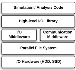
lay-Figure 1.1: I/O Software/Hardware Stack
outs and scenarios, including APLOD evaluation. We demonstrated a several-fold performance improvement for noncontiguous column vectors, 3D array slices, and 4D array subvolumes over CUDA-based alternatives. Compared with optimized, layout-specific implementations, our ap-proach incurs low overhead, while enabling the packing of datatypes that do not have a direct CUDA equivalent. These improvements are demonstrated to translate to significant improve-ments in end-to-end, GPU-to-GPU communication time. For APLOD in particular, we show that MPI-based solutions, whether within GPU or CPU memory, are not an efficient mapping of computation, necessitating other avenues of optimization.
1.2.3 Dynamic, Filesystem-level Data Layout Optimization
Consider the scientific software stack, shown in Figure 1.1. In general, data pre- and post-processing can be performed at numerous levels: application developers can manually incorpo-rate them into simulations, semantics can be added into the various I/O and communication middlewares that abstract the data processing, and filesystems can optimize access to modi-fied data formats. For example, compression has been integrated into I/O forwarding middle-ware [86, 115]), requiring no application-level modifications. As discussed, APLOD was orig-inally implemented as a combination of application-level and I/O library-level modifications, showing both I/O scalability and low transform overhead. However, HPC-centric, filesystem-level optimizations, taking advantage of the semantic qualities of distributed storage, have not been explored, leaving a number of research questions (such optimizations have been explored in other contexts; see Section 4.5).
Problems and Challenges
POSIX I/O) have not been explored, except indirectly through the typical filesystem tuning process and through I/O library configurations. There are opportunities for optimization at the filesystem level which requires answering pressing research questions. These research directions are driven by the shift towards more decentralized filesystem designs resembling HDFS [91] and GoogleFS [27], in order to continue to scale in terms of cost, reliability, and performance. Most importantly, the primary fault-tolerance mechanism in these systems is data replication. Significant performance improvements can be made by exploiting this form of fault-tolerance, tailoring different replications to different access patterns. From this goal, numerous research questions can be derived:
• What role does access semantics play in enabling access-pattern-based optimization and to what degree do we need to make these semantics available to the filesystem? As an APLOD example, different analysis scenarios require different degrees of data precision, implying different “optimal” layouts for the task at hand.
• How do we capture and optimize access patterns across replications in adynamicfashion? For example, the aggregate access patterns of initial analyses of data may not match those of later analyses. Furthermore, scientists may run many different analysis applications on a single dataset - static methodologies or optimizations driven locally, rather than globally, lack the flexibility needed to handle these cases.
• What effects do data reorganization have on maintaining synchronicity between different copies of the data? If there are non-trivial data transformations, then the modification of these copies of data is also non-trivial.
However, investigating these questions solely within the context of APLOD creates a mis-match in levels of abstraction: enabling and performing optimizations at the filesystem level specific to APLOD would have minimal impact on the larger storage community that is not applicable to other types of data layouts. Hence, we must consider higher-level problem ab-stractions to optimize using filesystem-level semantics, which can be applied to other problem domains (including APLOD).
Approach and Results
Not only can spatio-temporal data be represented as multidimensional matrices, but simulation variables themselves can be represented similarly. In databases, this distinction is made between a row-store, where each tuple is stored contiguously, and column-store, where each variable within a tuple is stored contiguously.
Given the likely future makeup of I/O systems, the use of data replication in parallel filesys-tems can be seen in three different contexts: a strict performance context, where data can be replicated to increase concurrent bandwidth to the file, aresilience context, where data can be recovered and accessible in case of system error (hardware or software), and an access pattern
context, where different replications can organize data to optimize various methods of access (such as row-major or column-major accesses). We initially focus our optimizations on the use of replications in the latter context, with the former two to be tackled in future work (see Chapter 5.1).
Optimizing these accesses in a dynamic fashion is a difficult problem, one requiring numerous steps. First, for the purpose of prototyping, we decompose the problem into two domains: a filesystem-level data layout scheme and a middleware-level replica management and I/O-driver (implemented as an MPI-IO extension). This allows us to experiment with replica layout policies and apply lessons-learned for future development of more tightly-integrated filesystem semantics with respect to replication. Second, we use the latest experimental developments in the PVFS filesystem [14, 31] to develop a direct, object-level data and replica layout policy, enabling a single container for all related data/metadata, all without modifying the original data layout in physical storage. Third, we develop an integrated tracer for MPI-IO capable of tracking collective optimizations, an important use case for I/O workloads, and utilize the IOSig trace analysis algorithm [11] to gather access-pattern information. Finally, we use a model-driven
approach to determine effective replica layouts for a given set of access-patterns and anaging mechanism based on frequency-of-access to prioritize replica decisions.
Chapter 2
Byte-precision Level of Detail
Processing for Variable Precision
Analytics
2.1
Introduction
Data reduction in extreme-scale, scientific simulations is a quickly emerging necessity to reduce current and especially future I/O bottlenecks, as compute performance continues to increase at a far higher rate than I/O performance [54]. I/O bottlenecks are especially pronounced when running analysis on simulation-generated data, a typically read-only process performed numerous times by multiple application scientists, often on dedicated analysis clusters with less computational power than the machines the data was generated on.
In the context of extreme-scale computing, data reduction technologies face a number of unique architectural, algorithmic, and application-specific challenges which complicate the emergence of an efficient solution that is highly applicable across application contexts. First, sci-entific data is notoriously hard-to-compress, due to the utilization of double-precision floating-point variables. These variables tend to have highly entropic mantissa bits, leading to data reduction only on the order of 10−30%. Achieving higher compression ratios with lossless compression methods require the discovery of non-trivial patterns within the typically spatio-temporal data, making these methods unsuitable for in-situ processing. While state-of-the-art lossless compression utilities such as ISOBAR [21] and FPC [10] have been making headway into fast lossless compression of scientific data, achieving high degrees of data reduction while retaining full precision is still best suited to a post-processing scenario, where a full-context approach is possible.
it more suitable for alleviating I/O bottlenecks in-situ. However, application scientists spend an enormous amount of effort ensuring accurate and precise simulation results. While the loss of precision may be acceptable for some simulations, it will not be for all.
Regardless of method, compression as a data reduction strategy introduces new, less optimal access patterns to the I/O system, on both a software and hardware level. On the software level, non-uniform compressed buffer sizes would necessitate global communication between I/O nodes, introducing additional latency costs. On the hardware level, applications optimized for certain striping patterns may lose performance due to the non-uniform buffer sizes, leading to disk contention and lost I/O bandwidth.
Given the challenges that data reduction impose for simulation codes, instead of focusing on reducing data at write-time, we argue it is highly beneficial to reduce data at read-time
through partial-precision analytics. The key insight here is that many types of analysis functions may produce acceptably accurate results even with a greatly reduced amount of precision. A common invocation of this principle can be found in multiresolution analysis (MRA) of wavelet-compressed data, traditionally used in the graphics and visualization communities. However, wavelet-based MRA has no bounds on errors at any resolution, and is technically not lossless for double-precision data (though it can be in some cases for single-precision data [104]). Furthermore, wavelet compression standards such as JPEG 2000 [99] have been successfully used to compress single-precision climate data [118], but requires the quantization of single-precision floating-point data, something which may not work well on double-precision datasets crossing a wide range of exponent values.
To achieve these ends, we propose aanalytics-driven precision level of detail (APLOD) pre-processing methodology. Our approach is inspired by the bit-level format of double-precision variables, and the fact that truncation of the mantissa component leads to low, bounded max-imum errors based on the number of mantissa bits kept (see Table 2.1). To promote high effi-ciency as well as application-specific tuning based on the accuracy needs of scientific simulation analyses, we enable a generalized partitioning of double-precision data along byte-boundaries, described by a byte-level component vector (CV). In other words, based on user preferences, datasets are partitioned into groups of contiguous significant bytes, such as the most significant two bytes. Datasets are stored contiguously by most significant bytes so that only data at a required level of precision can be loaded into memory. There are numerous benefits to this approach that, to our knowledge, have not been utilized by other analysis-level data-reduction methods:
MRA.
• APLOD processing minimally disturbs existing parallel I/O access patterns. If I/O pat-terns in an application are communication-free, then the patpat-terns with APLOD process-ing are communication free. Buffer sizes are deterministic, given the original data’s buffer sizes. The storage barrier to APLOD processing is low, requiring at most tweaking to disk striping parameters.
• APLOD processing is a low overhead operation in both theshuffling of a double-precision buffer to the decomposition defined by a CV as well as thereconstructionof the partitioned data back into original (or truncated) form. Even for the finest grain decomposition, the transform operations achieve a throughput of 600MB/s. Wavelet transforms, however, perform at a maximum of 434MB/s, which degrades significantly for very large buffers. When reconstructing partial-precision data from a packed significant byte representation, transform time is decreased in direct proportion with the data reduction. On a per-core basis, the transform throughput far exceeds hard disk bandwidth, making APLOD processing an ideal candidate forin-situ integration with applications.
• APLOD processing is orthogonal to existing data reduction and I/O optimization meth-ods. Lossless compression can be applied to each byte-component (oftentimes resulting in higher compression ratios [86]), and I/O optimizations exploiting data layout patterns need not be significantly changed to incorporate APLOD layout changes. Since wavelet MRA has stricter data layout requirements, applying complex layout optimizations to wavelet-transformed data can be nontrivial.
• The programming overhead required to express APLOD operations is minimal and simple to express using well-known I/O libraries, such as ADIOS [59].
Table 2.1: Maximum per-point percent errors on partial-precision IEEE 754 doubles, masking the remaining bytes with the quantity 0x7F···FF.
.
Significant Max Underest. Max Overest.
Bytes Error Error
2 -1.5e0% 3.1e0%
3 -6.1e-3% 1.2e-2%
4 -2.4e-5% 4.8e-5%
5 -9.3e-8% 1.9e-7%
6 -3.6e-10% 7.3e-10%
7 -1.4e-14% 2.8e-12%
2.2
Background
The concept of level of detail processing, or operating on a subset or approximation of the full context dataset, has been explored in numerous contexts. Examples include statistical sampling techniques, arising from the database community, I/O optimization frameworks in HPC that enable sampling on a spatio-temporal domain, and a wide range of signal and image processing techniques, using transforms such as various families of wavelets that enable MRA. Note that each level of detail processing method discussed is compatible with APLOD processing through applying the operations on each significant byte component, though seek costs, effects on wavelet accuracy, etc. need to be considered from the partitioning of byte-components.
Sampling in databases is a well-studied area, with much early work on general sampling queries [75, 72], sampling on an index [73], and sampling in spatial databases [74]. More recent work has also treated the issue of minimizing sampling error due to data skew [16, 32]. Database sampling methods typically do not change the underlying data layout, leading to a large number of seeks, a problem in HPC environments, where seeking in parallel file systems is a high-latency operation. Furthermore, statistical sampling runs the risk of losing small features or sharp transitions in the data, especially since most scientific datasets exist in some spatio-temporal domain. Finally, statistical sampling, such as random sampling, provides for data analysis errors as a distribution, rather than as a bound; while improbable, there is still the chance for significant skew depending on the data distribution.
hierarchi-cal data layouts. This method also provides a speed/accuracy tradeoff for data analysis, but has some potential drawbacks. Aside from the mentioned statistical sampling problems, the fixed sampling procedure of hierarchical data layouts is prone to selection bias, though for analysis operations such as visualization this is less of an issue.
Discrete wavelet transforms and MRA [23] are particularly popular for level of detail pro-cessing, commonly used in image standards such as JPEG 2000 [99] for high compression ratios while maintaining image integrity. In general, discrete wavelet transforms convert an input signal into detail coefficients (from a high-pass filter) and approximation coefficients (from a
low-pass filter), recursively transforming the approximation coefficients. The hierarchical nature of the transform allows reconstruction of the original signal from a subset of the approximation coefficients with high accuracy. Thus, wavelet MRA is the closest applicable method to our proposed APLOD processing. However, while low average errors from MRA are shown (see Section 2.4), there is no upper bound on the errors, and accuracy depends on spatio-temporal relationships in the data. Compared to APLOD, wavelet MRA allows for a much finer-grained decomposition of data. However, at least for the double-precision datasets we test on, using even one-half of the coefficients leads to unacceptable errors, rendering this capability mostly ineffective with such datasets.
2.3
Methodology
As mentioned, the goal of enabling efficient variable-precision analytics requires a modified data representation, one that is capable of being queried by varying degrees of precision. The reduced precision format should directly result in reduced I/O costs; otherwise, there is little tangible benefit to using such a representation aside from perhaps a reduced memory footprint. Furthermore, overhead for performing the transformation to and from the data representation must be small enough to not bottleneck the application.
Based on these restrictions and differing analysis needs of applications, we define a simple, parameterized data decomposition model based oncomponent vectors (CVs). We treat a buffer of data as a matrix of bytes, then define column slices (components) based on significant byte boundaries. These slices are transformed to occupy a contiguous buffer, which can then be read into memory separate from other levels of precision. CVs define these column slices, allowing users to choose a data decomposition that makes sense for their analysis needs.
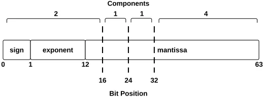
Figure 2.1: The partitioning of a IEEE 754 double-precision value by the CV {2,1,1,4}.
by double-precision data (not including subnormal values) is given by:
value = (−1)s×(1 +
52
X
i=1
(mi2−i))×2e−1023, (2.1)
wheresis the value of the sign bit, mi is each mantissa bit in decreasing order of significance,
and eis the unsigned integer interpretation of the exponent bits.
Given this representation, we make two observations that drive our partial-precision rep-resentation. First, we observe that the mantissa bits represent a fractional component in the overall value. That is, the entire mantissa component with the implicit one bit, between the minimum (of all zeroes) and maximum (of all ones), represents a factor in the resulting double-precision value in the range [1,2). Second, we observe that each less significant mantissa bit contributes an exponentially smaller amount to this multiplier. Given Equation 2.1, we can easily bound the effects of truncation or replacement of the mantissa bits, the results of which can be seen in Table 2.1.
Combined with the use of the exponent bits, truncation of the less significant mantissa bits thus provides a good opportunity to reduce the amount of data at small error rates. By comparison, truncation is typically not feasible for integer data since the bits encoding the integer are not exponentiated by a set of exponent bits. Given the double-precision format, the smallest byte-wise CV must always contain the exponent portion; otherwise, unacceptably high error rates would be generated. Hence, since we use byte-boundaries for efficiency reasons, the first component in any CV is restricted to be at least two bytes, as shown in Figure 2.1. As shown in Table 2.1, truncating to the most significant two bytes, along with masking the discarded mantissa bits, leads to a maximum relative error of 3.1%.
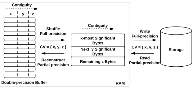
Figure 2.2: Byte-precision level of detail partitioning, based on a generic component vector (CV) splitting groups of significant bytes.
according to the needed level of precision. If necessary, the data is then reconstructed back to the original format, though with the missing significant bytes masked with an appropriate value to reduce the average error.
An example CV defined over a double-precision value is shown in Figure 2.1. For this CV ({2,1,1,4}), the first two bytes of each double-precision value are stored contiguously. As mentioned, these bytes contain the sign bit, all 11 exponent bits and the four most significant mantissa bits. If a buffer of size 8MB was being shuffled, the result would consist of four buffers: a buffer containing 2MB of most significant two bytes, two 1MB buffers of the next two significant bytes, and a 4MB buffer containing the remaining significant bytes.
2.3.1 Component Vector Representation and Operations
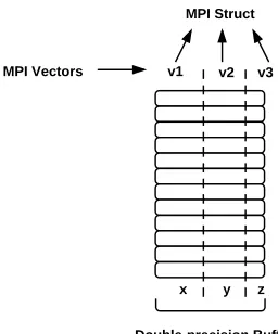
Figure 2.3: Partial-precision level of detail transformation using MPI datatypes, for CV {x, y, z}.
However, there are a number of issues with a purely MPI-based representation. First, the packing algorithm, which places the non-contiguous data into a contiguous buffer given a datatype specification, may not be efficient compared to a low-level implementation which can take advantage of vectorizing and loop unrolling. See Section 2.4.2. Second, in order to reconstruct at varying degrees of precision, it is necessary to create a different datatype per number of components to load. For example, for the CV {2,1,1,4}, four MPI structs need to be created, one for the first component, one for both the first and second components, and so on. Furthermore, when reconstructing partial-precision data, it is necessary to perform an additional memory setting operation to zero out or mask the significant bytes not loaded in, adding to the overhead. A specialized implementation is able to roll this memory set operation into the reconstruction process.
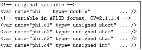
<!-- original variable -->
<var name="phi" type="double" ... />
<!-- variable in APLOD format, CV=2,1,1,4 --> <var name="phi.c1" type="unsigned short" ... /> <var name="phi.c2" type="unsigned char" ... /> <var name="phi.c3" type="unsigned char" ... /> <var name="phi.c4" type="unsigned int" ... />
Figure 2.4: A double-precision variable in the ADIOS XML configuration, in both unmodified and in APLOD format.
2.3.2 Partial-precision I/O
While it is difficult to provide a generic I/O analysis for each simulation code, there exist a number of parallel I/O middlewares that abstract file storage details from the application while ensuring high performance. A particularly popular I/O abstraction is the Adaptable I/O System (ADIOS) [59]. ADIOS is a state-of-the-art componentization of the I/O system that, with a simple change to an entry in an XML configuration file, changes codes to use numerous I/O backends, called “transports,” without requiring application recompilation. For example, POSIX, MPI-IO, parallel HDF5 [120], PnetCDF [56], and numerous others are supported trans-ports. Given the flexibility of I/O methods to use and the possibility for defining the CV through the XML configuration file, we chose to use ADIOS to show that data reduction through our partial precision reorganization of data can translate directly to improved I/O costs, and can do so under a wide range of application contexts.
Enabling APLOD processing using ADIOS requires two simple changes. The first change is at the configuration level, where the ADIOS XML configuration file is modified to support the retrieval of partial-precision data. Figure 2.4 shows an example. For each variable being reorganized using APLOD, new variables are created for each CV component to replace the original variable. For multivariate data, there are two ways to place the CV components in the configuration file. The first is to interleave the CV components for each variable, optimizing the access of multiple variables at a particular degree of precision in one fell swoop. The other is to place all CV components consecutively for each variable, optimizing for univariate access of data at various degrees of precision.
2.4
Experimental Evaluation
To evaluate the APLOD methodology in a leadership-class HPC environment, we perform all experiments on Oak Ridge National Laboratory’s Jaguar cluster (Cray XK6 architecture), consisting of a single 16-core AMD Opteron 6200 processor and 32GB of memory per node. For I/O benchmarks, we use ADIOS version 1.3.1 on the Lustre parallel file system.
We look at datasets from a number of real-world simulations. GTS [111] and XGC-1 [82] are both particle-in-cell simulations of nuclear fusion devices, with GTS studying microturbulence in the plasma core and XGC-1 studying microturbulence at the edge. We examine thepotential
(φ) variable of a single timestep from GTS and the temperature varaible of a single timestep from XGC-1. Finally, we look at S3D [17], a direct numerical simulation of reacting flows in combustion. We examine thevelocity variable of a single timestep in two dimensions (uvel and
vvel).
As a primary source of comparison, we use wavelet multiresolution analysis. Specifically, we use the D4 Daubechies wavelet provided by the GNU Scientific Library (GSL) [25]. Compared to the other wavelet options available in the GSL (such as Haar and Spline), the D4 wavelet was the most accurate for the datasets used in this paper and had minimal performance differences. For the GTS potential variable, which is linearized from a toroidal structure, we use the one-dimensional wavelet transform. For the other two-and-three-one-dimensional datasets, we divide the data spatially into 32×32 blocks and use the standard two-dimensional transform on each, which interleaves each level of the transform between rows and columns. For comparison against APLOD reorganization, we then load the most significant wavelet coefficients and reconstruct the data, replacing with zeroes the remaining coefficients.
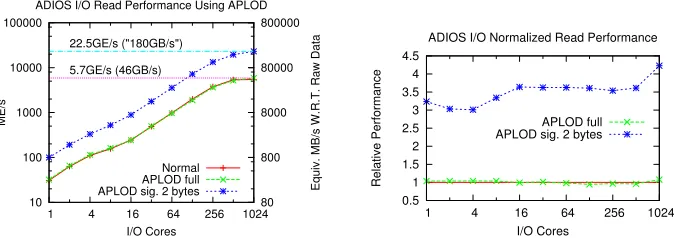
10 100 1000 10000 100000
1 4 16 64 256 1024
80 800 8000 80000 800000
ME/s
Equiv. MB/s W.R.T. Raw Data
I/O Cores
ADIOS I/O Read Performance Using APLOD
5.7GE/s (46GB/s) 22.5GE/s ("180GB/s")
Normal APLOD full APLOD sig. 2 bytes
0.5 1 1.5 2 2.5 3 3.5 4 4.5
1 4 16 64 256 1024
Relative Performance
I/O Cores
ADIOS I/O Normalized Read Performance
APLOD full APLOD sig. 2 bytes
Figure 2.5: Parallel I/O read performance (actual and relative) using ADIOS, with and without APLOD-reorganization. ME/s - millions of elements per second. GE/s - billions of elements per second.
induce, in effect keeping the data in as close to original form as possible.
2.4.1 I/O Performance
Using ADIOS as a driver for our APLOD I/O performance benchmarking, we investigate parallel read performance under a number of scenarios. On a per-reader basis, we chose a partition size of 512MB for two reasons: first, data reading scenarios tend to use many less cores than writing for analysis purposes due to different resource allocation for the respective tasks, and second, we wish to target bandwidth-bound analysis scenarios, and thus minimize the effect of access latency. Furthermore, we chose to test on the CV{2,1,1,4}, as our accuracy results in Section 2.4.3 indicate that the first four bytes of double-precision variables are sufficient to perform many types of analysis operations, while the latter four bytes are used where full precision is needed (e.g., checkpoint-restart data).
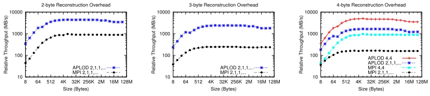
2.4.2 Transform Performance
For a number of CVs, we test APLOD transformation performance using both our manual implementation and the MPI datatypes representation. For each benchmark, we measure the slowest possible transformation, corresponding to the finest grain CV{2,1,1,1,1,1,1}, as well as a few others, to show the effect of partitioning with varying degrees of coarseness on transform overhead.
Furthermore, we compare against the one-dimensional transform provided by the GSL for a few reasons. Most notably, the output format of the one-dimensional transform may be directly used for multiresolution analysis and is thus most applicable for comparison against APLOD. The two-dimensional transform, in order to support the contiguous layout of each “level” of the transform, would require additional data reorganization. Combined with the need to transform non-contiguous column data, the overhead becomes unacceptably large.
10 100 1000 10000
8 64 512 4K 32K 256K 2M 16M 128M
Throughput (MB/s) Size (Bytes) Shuffle Performance A 4,4 A 2,1,1,4 A 2,1,1,1,... Wav-1D M 4,4 M 2,1,1,4 M 2,1,1,1... 10 100 1000 10000
8 64 512 4K 32K 256K 2M 16M 128M
Throughput (MB/s)
Size (Bytes) Full-precision Reconstruct Performance
A 4,4 A 2,1,1,4 A 2,1,1,1,... Wav-1D M 4,4 M 2,1,1,4 M 2,1,1,1,...
Figure 2.6: Performance of transforming from original data layout to component-level con-tiguous chunks, and vice versa. A - APLOD.M - MPI datatypes. Wav-1D - one-dimensional wavelet transform.
10 100 1000 10000
8 64 512 4K 32K 256K 2M 16M 128M
Relative Throughput (MB/s)
Size (Bytes) 2-byte Reconstruction Overhead
APLOD 2,1,1,... MPI 2,1,1,... 10 100 1000 10000
8 64 512 4K 32K 256K 2M 16M 128M
Relative Throughput (MB/s)
Size (Bytes) 3-byte Reconstruction Overhead
APLOD 2,1,1,... MPI 2,1,1,... 10 100 1000 10000
8 64 512 4K 32K 256K 2M 16M 128M
Relative Throughput (MB/s)
Size (Bytes) 4-byte Reconstruction Overhead
APLOD 4,4 APLOD 2,1,1,... MPI 4,4 MPI 2,1,1,...
Figure 2.7: Performance of partial-precision value reconstruction.
2.4.3 Partial Precision Analysis Accuracy
Basic Measures
While the benefits of partial precision analysis to I/O costs are clear and intuitive, it must be verified that partial precision analytics is a viable methodology to pursue. More specifically, it is necessary to determine at which levels of precision analysis functions provide adequately accurate results. As the scope of analysis functions on scientific data is much too large for an exhaustive survey, we choose a number of simple and more complex analysis scenarios to determine the potential for large-scale partial-precision analytics.
Table 2.2: Per-point relative errors (absolute values).
Per-point relative error (%, absolute)
Median Maximum
Variable Parameter1 APLOD D4 APLOD D4
2 1.08e0 1.10e1 3.12e0 2.12e6
potential 3 4.24e-3 - 1.22e-2
-4 1.65e-5 4.55e0 4.76e-5 5.57e5
2 1.02e0 1.30e-1 3.12e0 7.10e1
temp 3 4.24e-3 - 1.21e-2
-4 1.63e-5 5.34e-2 4.73e-5 4.08e1
2 1.08e0 4.44e-2 3.12e0 3.84e5
uvel 3 4.15e-3 - 1.22e-2
-4 1.62e-5 1.23e-2 4.77e-5 1.31e5
2 1.08e0 6.34e-1 3.12e0 1.30e7
vvel 3 4.24e-3 - 1.22e-2
-4 1.66e-5 1.87e-1 4.77e-5 2.26e6
1
Proportion of data used. For APLOD, the number of significant bytes. For the D4 wavelet, the proportion of coefficients brought in for multiresolution analysis, as a fraction of eight.
standard deviation values and near equivalent (1.0) Pearson correlations. Furthermore, the average absolute relative error per-point is low, though the maximum error for two bytes of precision reaches the maximum possible. In comparison, the wavelet-reconstructed data has much more variability. The most significant difference between the D4 wavelet and APLOD is the presence of large relative errors in the wavelet-reconstructed data, that persist even for a large number of coefficients. Also, the errors seen in the wavelet-regenerated data see a lesser degree of change when moving from lower precisions to higher precisions, both due to the “vanishing” nature of the less significant coefficients as well as the persistence of high maximum errors throughout.
Distributional Analysis: k-means and Histogram
Since there is little error between points of data, and that error is distributed across the dataset, the previous metrics were expected to be highly accurate. However, small changes to a variable may change the global behavior of analysis algorithms that, for example, partition the data. In the worst case, edge conditions between the partitions can be sensitive to changes in precision, producing different results. To test the possibility of small local changes yielding large global changes, we performed two experiments on the data: generating an equal-interval histogram based on the data with a constant number of bins, and clustering the data via the k-means algorithm with randomized centroids.
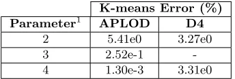
Table 2.5 show the misclassification rate of running the k-means algorithm on the uvel
Table 2.3: Pearson Correlation between full and partial-precision data.
Pearson Correlation
Variable Parameter1 APLOD D4
2 1-8.59e-5 0.972
potential 3 1-1.34e-9
-4 1-0.00e0 0.996
2 1-5.75e-04 0.954
temp 3 1-9.04e-09
-4 1-1.34e-13 0.984
2 1-6.59e-04 0.992
uvel 3 1-9.97e-09
-4 1-4.77e-14 0.998
2 1-9.27e-05 0.993
vvel 3 1-1.42e-09
-4 1-0.00e0 0.998
1
Proportion of data used. For APLOD, the number of significant bytes. For the D4 wavelet, the proportion of coefficients brought in for multiresolution analysis, as a fraction of eight.
Table 2.4: Partial-precision relative errors for mean and standard deviation.
Mean Error (%) Std. Dev. Error (%)
Variable Parameter1 APLOD D4 APLOD D4
2 3.88e0 1.60e-11 5.53e-2 2.77e0
potential 3 2.88e-2 - 2.70e-5
-4 2.06e-4 9.78-11 1.54e-7 4.24e-01
2 6.87e-2 7.91e-14 2.92e-1 4.64e0
temp 3 6.46e-6 - 1.87e-4
-4 4.57e-8 9.10e-13 1.56e-9 1.64e0
2 1.90e-2 8.47e-12 9.85e-2 8.16e-1
uvel 3 3.81e-6 - 1.95e-5
-4 4.64e-9 1.27e-11 1.39e-8 2.09e-1
2 4.26e-2 2.68e-12 6.30e-2 6.90e-1
vvel 3 1.04e-5 - 6.80e-6
-4 2.30e-8 3.64e-12 5.81e-8 1.55e-1
1Proportion of data used. For APLOD, the number of significant bytes. For the D4 wavelet, the proportion of
Table 2.5: Clustering errors, measured as the misclassification rate compared to full-precision. The uvel and vvel variables from S3D are partitioned into 10 clusters.
K-means Error (%)
Parameter1 APLOD D4
2 5.41e0 3.27e0
3 2.52e-1
-4 1.30e-3 3.31e0
1Proportion of data used. For APLOD, the number of significant bytes. For the D4 wavelet, the proportion of
coefficients brought in for multiresolution analysis, as a fraction of eight.
centroids for both the full and partial precision data and computing the proportion of partial-precision points assigned to different clusters than the corresponding full partial-precision points. For two bytes of precision, 5.41% of points are assigned to a different cluster than when using full-precision values. These points are likely near the “edges” of the original clusters, which are vulnerable to membership switching through small changes in the cluster centers. The error quickly disappears when using a higher degree of precision, however. Once again, in the wavelet-reconstructed data we see a relatively consistent level of error due to the existence of outliers. At the lowest degree of precision tested, the error is less than that of APLOD, but the persistent presence of outliers regardless of the proportion of wavelet coefficients keeps the errors relatively consistent, while increasing the bytes of precision with APLOD quickly overcomes such errors. Figure 2.8 superimposes the partial-precision histogram on the full-precision version. We display only the XGC-1 temperature histogram as it is the most illustrative of the trends shown in the datasets considered (S3D has similar patterns, but to a lesser degree, and the exponential component of GTS data differs by far too much for a equal-interval histogram to capture useful distributional information). Note that the selection of data we are using has little difference in the exponential component, meaning that the fractional component is a relatively more important component of the data.
For APLOD-based reconstruction, as Figure 2.8 shows, the problems with losing precision (truncating the six least significant mantissa bytes) are apparent. There is a clear “clustering” effect whereby there is not enough precision to sufficiently separate values into bins when equal-interval binning is used, hence the oscillatory pattern between empty bins and much larger bins. One solution is to use different parameters based on the degree of precision used, which is undesirable; ideally, reduced precision should only introduce noise into the analysis, instead of requiring a revisiting of the analysis function. In any case, with three bytes of precision, these problems all but disappear, suggesting that three bytes is accurate enough to represent this dataset. Data with small ranges that primarily occupy the mantissa portion of the double-precision data are likely to need additional double-precision.
0 200 400 600 800 1000 1200 1400
0 20 40 60 80 100
Frequency
Bin
XGC temp Histogram by Precision Full 2-byte 0 200 400 600 800 1000 1200 1400
0 20 40 60 80 100
Frequency
Bin
XGC temp Histogram by Wavelet MRA Full 1/4 MRA 0 200 400 600 800 1000 1200 1400
0 20 40 60 80 100
Frequency
Bin
XGC temp Histogram by Precision
Full 3-byte 0 200 400 600 800 1000 1200 1400
0 20 40 60 80 100
Frequency
Bin
XGC temp Histogram by Wavelet MRA Full 1/2 MRA
Figure 2.8: XGC-1 100-bin histograms.
that the APLOD data has. Figure 2.8 shows that the existence of outliers shift the range of the data, leading to a different distribution of values among them. However, even if the bins were “shifted” from lower to higher bins in Figure 2.8, skewed results would still appear, as evidenced in the spikes in values compared to the three bytes of precision in APLOD, which matches perfectly against the full-precision data.
Fourier Analysis Accuracy
Finally, some analysis functions involve transformations of the data into a different space. In particular, many applications rely on signal processing techniques for data analysis, built on transformations such as wavelet and Fourier transforms. The data in this case may be especially prone to error propagation since new points of data are produced by sometimes complex operations on the full or subselected data set, which are then analyzed.
For GTS simulations in particular, Fourier Transforms (FFT) of the grid-based electrostatic potential are carried out to analyze the spectral characteristics of turbulence in the fusion core. Gradients in the hot fusion plasma generate so-called “drift waves”, which couple with each other through non-linear effects. Charged particles forming the plasma continuously exchange energy with these waves as turbulence develops. Spectral analysis through FFTs allows the identification of the most important modes in the system (i.e., fastest growing modes) and how they couple with each other to form other modes.
numbers, we generated three metrics for both APLOD and wavelet MRA. First, we organize the data by drift wave number and calculate the mean/median relative error vs. the full-precision-generated FFT data, to examine if there is a distributional relation between the errors. Second, we plot the absolute values of the full-precision FFT coefficients against the corresponding error seen to examine whether there is a relation between exponent value and error. Figures 2.9 and 2.10 show these metrics for the wavelet-generated and APLOD data, respectively, while Table 2.6 gives a numerical distribution of the errors. The real component is shown for these metrics; in comparison, the complex component shows similar trends and the magnitude of the complex numbers shows order-of-magnitude improvements in accuracy.
1e+02 1e+04 1e+06 1e+08 1e+10 1e+12 1e+14 1e+16
0 200 400 600 800 1000 1200
Mean Relative Error (%)
Wave Number Mean Errors Real Comp. (1/2 Wav. Coeff.)
error = 1% error = 5% error = 10% error = 100%
1e+00 1e+02 1e+04 1e+06 1e+08 1e+10 1e+12 1e+14
0 200 400 600 800 1000 1200
Mean Relative Error (%)
Wave Number Median Errors Real Comp. (1/2 Wav. Coeff.)
error = 1% error = 5% error = 10% error = 100%
1e+00 1e+05 1e+10 1e+15
1e-20 1e-16 1e-12 1e-08
Mean Relative Error (%)
FFT Real Component Abs. Value 1/2 Wavelet Coeff. Errors vs. Real Component
error = 1% error = 5% error = 10% error = 100%
a b c
Figure 2.9: For the D4 wavelet, a,b - Mean, median errors of FFT data along each drift wave (real component), and c- FFT errors plotted against real component value.
1e+00 1e+02 1e+04 1e+06 1e+08 1e+10 1e+12 1e+14 1e+16
0 200 400 600 800 1000 1200
Mean Relative Error (%)
Wave Number Mean Errors Real Comp. (2-byte Precision)
error = 1% error = 5% error = 10% error = 100%
1e+00 1e+01 1e+02
0 200 400 600 800 1000 1200
Mean Relative Error (%)
Wave Number Median Errors Real Comp. (2-byte Precision)
error = 1% error = 5% error = 10% error = 100%
1e-10 1e-05 1e+00 1e+05 1e+10 1e+15 1e+20
1e-20 1e-16 1e-12 1e-08
Mean Relative Error (%)
FFT Real Component Abs. Value 2-byte Partial Precision Errors vs. Real Component
error = 1% error = 5% error = 10% error = 100%
1e-02 1e+00 1e+02 1e+04 1e+06 1e+08 1e+10 1e+12 1e+14
0 200 400 600 800 1000 1200
Mean Relative Error (%)
Wave Number Mean Errors Real Comp. (3-byte Precision)
error = 1% error = 5% error = 10% error = 100%
1e-03 1e-02 1e-01 1e+00
0 200 400 600 800 1000 1200
Mean Relative Error (%)
Wave Number Median Errors Real Comp. (3-byte Precision)
error = 1% error = 5% error = 10% error = 100%
1e-10 1e-05 1e+00 1e+05 1e+10 1e+15
1e-20 1e-16 1e-12 1e-08
Mean Relative Error (%)
FFT Real Component Abs. Value 3-byte Partial Precision Errors vs. Real Component
error = 1% error = 5% error = 10% error = 100%
1e-04 1e-02 1e+00 1e+02 1e+04 1e+06 1e+08 1e+10 1e+12
0 200 400 600 800 1000 1200
Mean Relative Error (%)
Wave Number Mean Errors Real Comp. (4-byte Precision)
error = 1% error = 5% error = 10% error = 100%
1e-05 1e-04 1e-03
0 200 400 600 800 1000 1200
Mean Relative Error (%)
Wave Number Median Errors Real Comp. (4-byte Precision)
error = 1% error = 5% error = 10% error = 100%
1e-10 1e-05 1e+00 1e+05 1e+10
1e-20 1e-16 1e-12 1e-08
Mean Relative Error (%)
FFT Real Component Abs. Value 4-byte Partial Precision Errors vs. Real Component
error = 1% error = 5% error = 10% error = 100%
a b c
Figure 2.10: For varying APLOD precisions, a,b - Mean, median errors of FFT data along each drift wave (real component), andc - FFT errors plotted against real component value.
2.5
Conclusion
Table 2.6: Distribution of relative errors for real, complex, and magnitude components of FFT data generated from the GTS phi data. Total number of points is 191751. Arefers to APLOD,
W refers to wavelets, and the number refers to the proportion of the full dataset used (as a fraction of eight).
Comp. Rel. Err. (%) A-2 A-3 A-4 W-4
Real
x≤1 27912 177681 191558 752
1< x≤5 36193 10235 92 3041
5< x≤10 22306 1688 10 3632
10< x≤100 77202 1789 10 66114
100≤x 28138 358 81 118212
Complex
x≤1 32420 179648 191547 719
1< x≤5 43955 8887 88 2969
5< x≤10 23652 1322 14 3802
10< x≤100 67067 1525 8 65491
100≤x 24657 369 94 118770
Magnitude
x≤1 52841 190283 191751 1445
1< x≤5 60856 1410 0 6086
5< x≤10 26606 44 0 7534
10< x≤100 46830 12 0 122837
100≤x 4618 2 0 53849
Chapter 3
Enabling Fast, Noncontiguous GPU
Data Movement in Hybrid
MPI+GPU Environments
3.1
Introduction
A great amount of interest in the HPC community has been centered on the capabilities of graphics processing units (GPUs) as inexpensive, many-core accelerators. Evidence of this is seen in recent Top500 lists of supercomputers [1], where GPU accelerators are gaining in popu-larity due to their effectiveness over a wide range of computational loads and a favorable FLOPs to power ratio.
A number of technical challenges arise from the addition of a fundamentally different com-puting architecture to existing systems. Aside from the cost of developing, porting, and optimiz-ing codes to run on the GPU, there is a greater concern about integratoptimiz-ing them into algorithms with non-trivial point-to-point and collective communication patterns. The currently prevailing GPU accelerator model consists of discrete graphics processing hardware with memory separate from the CPU’s RAM. Hence, any communication operation involving data resident in GPU memory requires moving data between GPU and CPU memories, effectively adding another “hop” to the communication graph. Since the MPI Standard [65] does not define MPI’s inter-action with GPU memory managed by, for example, OpenCL [43] or CUDA [71], the burden of managing distinct memory spaces, especially of non-contiguous communication, falls on the application developers.