R E S E A R C H
Open Access
Deterministic construction of Fourier-based
compressed sensing matrices using an almost
difference set
Nam Yul Yu
*and Ying Li
Abstract
In this paper, a new class of Fourier-based matrices is studied for deterministic compressed sensing. Initially, a basic partial Fourier matrix is introduced by choosing the rows deterministically from the inverse discrete Fourier transform (DFT) matrix. By row/column rearrangement, the matrix is represented as a concatenation of DFT-based submatrices. Then, a full or a part of columns of the concatenated matrix is selected to build a newM×Ndeterministic
compressed sensing matrix, whereM=prandN=L(M+1)for primep, and positive integersrandL≤M−1. Theoretically, the sensing matrix forms a tight frame with small coherence. Moreover, the matrix theoretically guarantees unique recovery of sparse signals with uniformly distributed supports. From the structure of the sensing matrix, the fast Fourier transform (FFT) technique can be applied for efficient signal measurement and reconstruction. Experimental results demonstrate that the new deterministic sensing matrix shows empirically reliable recovery performance of sparse signals by the CoSaMP algorithm.
1 Introduction
Compressed sensing (or compressive sampling) is a novel and emerging technology with a variety of applications in imaging, data compression, and communications. In com-pressed sensing, one can recover sparse signals of high dimension from incomplete measurements. Mathemati-cally, measuring anN-dimensional signalx∈RN with an
M×Nmeasurement matrixyields anM-dimensional
vectory = x, whereM < N. Imposing a requirement
thatxiss-sparse or the number of nonzero entries inxis at mosts, one can recoverxexactly with high probabil-ity by anl1-minimization method or a greedy algorithm,
which is computationally tractable.
Many research activities have been triggered on the-ory and practice of compressed sensing since Donoho, Candes, Romberg, and Tao published their marvelous theoretical works [1-3]. The efforts revealed that a mea-surement matrixplays a crucial role in recovery ofs -sparse signals. Although a random matrix provides many theoretical benefits [4], it has the drawbacks [5] of high
*Correspondence: [email protected]
Department of Electrical and Computer Engineering, Lakehead University, Thunder Bay, Ontario P7B 5E1, Canada
complexity and large storage in its practical implementa-tion. As an alternative, we may consider adeterministic matrix, where well-known codes and sequences have been employed for the construction, e.g., chirp sequences [6], Alltop sequences [7,8], Kerdock and Delsarte-Goethals codes [9], second-order Reed-Muller codes [10], and BCH codes [11]. Other techniques for deterministic construc-tion, based on finite fields, representation theory, charac-ters and algebraic curves, and multicoset codes, can be also found in [12-18]. The deterministic matrices guaran-tee the recovery performance that is empirically reliable, allowing fast processing and low complexity.
In this paper, we study deterministic construction of a new class of Fourier-based compressed sensing matri-ces. Initially, apr×(p2r−1)basic partial Fourier matrix, equivalent to the partial Fourier codebook of [19], is intro-duced by selectingprrows from the(p2r−1)-point inverse discrete Fourier transform (DFT) matrix according to an
almost difference set, where p is a prime number and
r is a positive integer. By rearranging the rows and/or columns, we show that the matrix is represented as a con-catenation of DFT-based submatrices. Then, a full or a part of columns of the concatenated matrix is selected
to build a newM×N sensing matrix for deterministic
compressed sensing, whereM = pr andN = L(M+1)
forL ≤ M− 1. The concatenated structure allows the
new sensing matrix to offer the various admissible column numbers while keeping it as an incoherent tight frame and enables efficient processing for measurement and recon-struction in compressed sensing. We would like to stress that it is not a trivial task to obtain the concatenated struc-ture from the basic partial Fourier matrix by row/column
rearrangement. With the parameters MandN, our new
deterministic matrix can achieve the various permissible compression ratios of MN ≈ L1 for a positive integer L,
2≤L≤M−1.
Theoretically, the new sensing matrix forms a tight frame with small coherence. Moreover, our new sens-ing matrix theoretically guarantees unique recovery of sparse signals with uniformly distributed supports with high probability. From the structure of our new sensing matrix, the fast Fourier transform (FFT) technique can be applied for efficient signal measurement and recon-struction. Experimental results demonstrate that the new deterministic compressed sensing matrix, together with the CoSaMP recovery algorithm [20], empirically guar-antees sparse signal recovery with high reliability. We observe that the empirical recovery performance of our new sensing matrices is similar to those of chirp sens-ing [6] and random partial Fourier matrices. However, our new matrices offer several practical benefits, requiring less storage and complexity than random partial Fourier
matrices and providing more parameters ofMandNthan
chirp sensing codes.
The rest of this paper is organized as follows. In Section 2, we introduce basic concepts and notations to understand this work. Section 3 modifies the struc-ture of a basic partial Fourier matrix and presents a new sensing matrix for deterministic construction. We also discuss the efficient implementation and the the-oretical recovery guarantee of the new sensing matrix. Section 4 describes the signal measurement process and the CoSaMP recovery algorithm by employing the FFT technique. In Section 5, we demonstrate the empirical recovery performance of our new sensing matrices in noiseless and noisy settings. Finally, concluding remarks will be given in Section 6.
2 Preliminaries
This section introduces fundamental concepts and nota-tions for understanding this work. In subsecnota-tions 2.1 and 2.2, we briefly introduce the concepts of finite fields, trace functions and cyclotomic cosets for signal processing researchers. For more details, see [21] and [22].
2.1 Finite fields and trace functions
Letpbe prime andm>1 a positive integer. Afinite field Fpm is generated by 0 and αi,i = 0, 1,. . .,pm −2, i.e.,
Fpm = {0, 1,α,α2,. . .,αp m−2
}, whereαis called a primi-tive elementandαpm−1=1. The primitive elementαis a root of a primitive polynomialf(x), i.e.,f(α)= 0, where f(x)has the highest degreemand its coefficients are the elements ofFp= {0, 1, 2,. . .,p−1}.
Let k be a positive integer that divides m. A trace
function is a linear mapping fromFpmontoF
pkdefined by
Trmk(x)= m/k−1
i=0
xpki, x∈Fpm
where the addition is computed modulop. The trace func-tion algebraically defines the well-knownm-sequencesor pseudo-noise (PN) sequences, which have been widely used
in wireless communications. For instance, ifp = 2 and
k=1, then(Trm1(1), Trm1(α), Trm1(α2),. . ., Trm1(α2m−2))is a binarym-sequence of length 2m−1, where each entry is 0 or 1. Them-sequence, defined by a trace function, is effi-ciently generated by alinear feedback shift register (LFSR), which is a common method in communication standards.
Example 1. Letp= 2 andm= 4. Then, the finite field F24is defined by a primitive polynomialf(x)=x4+x+1,
where the rootαis a primitive element ofF24. Thus,F24 =
{0, 1,α,α2,. . .,α14}, whereα4+α+1 =0 andα15 =1. The trace function Tr41(x)takes on either 0 or 1, since it is a linear mapping fromF24ontoF2. For example,
Tr41(1)=1+1+1+1=0,
Tr41(α)=α+α2+α4+α8=0,
Tr41(α3)=α3+α6+α12+α9=1
where the addition is computed modulop=2.
2.2 Cyclotomic cosets
LetZv = {0, 1,. . .,v−1}, wherevis a positive integer. Also,pis a prime integer which is relatively prime tov, i.e., gcd(v,p) = 1. For a nonnegative integer s ∈ Zv, a
cyclotomic cosetmodulovoverpcontainingsis defined as
Cs= {s,sp,sp2,. . .,spns−1}
wherensis the smallest positive integer such thatspns ≡
Example 2.Letp=2 andv=15. Then, the cyclotomic
2.3 Basic partial Fourier matrixA
In this subsection, we introduce a basic framework from which a new sensing matrix can be developed in Section 3.
Throughout this paper, we set M = pr and N =
p2r − 1 = M2 − 1 for prime p and a positive
inte-ger r. Also, we assume that each column of a sensing
matrix has unitl2-norm, where thel2-norm is denoted
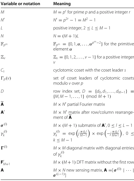
as||x|| = n−i=01|xi|2for ann-dimensional vectorx = (x0,x1,. . .,xn−1). Table 1 summarizes all the variables and
notations for the development of a new sensing matrix. In [19], Yu, Feng, and Zhang presented a new class of (N,M)near-optimal partial Fourier codebooks using an almost difference set [23]. The codebook can be equiva-lently translated into anM×N partial Fourier matrix, which containsMrows selected from theN-point inverse DFT (IDFT) matrix according to the almost difference set.
Table 1 Variables and notations for the new sensing matrix
Variable or notation Meaning
Cs cyclotomic coset with the coset leaders
p(v) set of coset leaders of cyclotomic cosets modulovoverp
D row index set,D = {d0,d1,. . .,dM−1} ≡
{M,M−1,. . ., 1} (modM+1)
A M×Npartial Fourier matrix
A M×Nmatrix after row/column rearrange-ment ofA
(l) M×Mdiagonal matrix with diagonal entries ofγk(l)
FM+1 M×(M+1)DFT matrix without the first row A M×Nnew sensing matrix,A=[σ(0)| · · · |
σ(L−1)]
From the results of [19], Proposition 1 describes the basic partial Fourier matrix and its geometric properties with the notations of this paper.
Proposition 1.For prime p and a positive integer r,
let M = pr and N = p2r − 1 = M2− 1. Let D =
{d0,d1,. . .,dM−1}be an index set defined in Lemma 2 of
[19], which will be given below in Remark 1. Choosing M rows from the N-point IDFT matrix according to D, we construct an M×NmatrixA, where each entry is given by
transpose of its complex conjugate. The coherence nearly achieves the Welch bound equality [25] of
N−M M(N−1) ≈
1 √
M+1 for sufficiently large M. Moreover,Aforms a tight
frame [26] as each row is mutually orthogonal.
The coherence and the tightness ofAdo not change if we select the rows from the DFT matrix, instead of the IDFT matrix. In this paper, we decide to use the IDFT matrix.
Remark 1.With the notations of this paper, the row
index setDis defined by [19]
D= {(M+1)ev−v|v∈I} where
where all the operations inDare computed moduloN. In Equation 1,Dis an almost difference set, andevis a non-negative integer satisfyingα(pr+1)ev = Tr2r
r (αv)forv ∈ I [19], whereαis a primitive element inFp2r. To determine the index setD, one needs to compute ev using a trace function, which might be difficult for signal processing researchers. In Section 3, we will present an alternative method to generate the indices ofDby successive multi-plication to predetermined values, which does not require the computation ofev. Therefore, it suffices to assume that
evis simply an integer in this paper.
3 Construction of new Fourier-based sensing matrices
To build a newM×Nsensing matrix, we begin with the
the N columns after a row/column rearrangement. Our approach is different from a conventional one of random
or deterministic selection of M rows out of an N × N
Fourier matrix, but we will show that it ultimately presents reliable recovery performance and practical benefits in implementation.
In deterministic compressed sensing, it is desired that a sensing matrix should be able to support a variety of admissible column numbers to sense a signal of various lengths. For this purpose, one needs to consider how to select the columns fromAfor a newM×Nsensing matrix with N < N. In this section, we apply a row/column permutation to the partial Fourier matrixAto obtain its
variant M× N matrix A. Then, we choose a full or a
part of columns ofAto construct a newM×N sensing
matrixA, whereN = (M+1)Lfor a positive integerL,
2 ≤ L ≤ M−1. The row/column rearrangement offers
the following benefits for our new sensing matrix A in
compressed sensing, which is the motivation:
1. If one selects the columns arbitrarily fromA, the resulting sensing matrix may not be a tight frame in general. In fact, one needs to be careful in selecting the columns ofA, to achieve the tightness of the resulting matrix. Through the row/column rearrangement, we will show that the new sensing matrixAhas aconcatenated structure of(M+1) -point DFT-based submatrices. With the structure,A can be still a tight frame by choosingN as a multiple ofM+1, which will be shown in Lemma 2.
2. The concatenated structure ofAalso allows efficient (M+1)-point FFT processing for measurement and recovery of sparse signals in compressed sensing. Note that if one selects the columns arbitrarily from the originalA, the resulting matrix generally requires theN-point FFT processing, which has more computational complexity. Moreover, one may enjoy fast processing via parallel FFT computations using the concatenated structure, which will be discussed in Section 4.
3.1 Structure
Recall the partial Fourier matrix A in Proposition 1. If p=2, we use the original index setDin Equation 1, i.e.,
D= {(M+1)ev−v|v∈ZM+1\ {0}}. (2)
On the other hand, ifp> 2, we redefine the index setD by adding M+21to each original index in Equation 1, i.e.,
D=
The above modification forp>2 ensures that each entry
of Dis nonzero when computed moduloM+1, which
also holds forp = 2. See the proof of Lemma 1 for the
implication.
Now, we suggest a column rearrangement of the original
Next, we show that the submatrixσ(l)has a DFT-based structure if the row indices ofDare arranged in appropri-ate order. In Lemma 1, we denoteFM+1as theM×(M+1) DFT matrix without the first row, where each entry is Fk,t=exp−j2π(M+k+11)tfor 0≤k≤M−1 and 0≤t≤M.
which clearly shows the DFT-based structure ofσ(l).
Proof. We investigate how expj2πdkt
M+1
Case. p = 2: In this case, each element of D in Equation 2 is represented as
dk=(M+1)ek+1−(k+1)≡ −(k+1) (modM+1)
in Equation 4. Consequently, each entry of Equation 4 forms anM×(M+1)submatrixσ(l)where each row is from the(M+1)-point DFT matrix excluding all one row and then masked byγk(l). Then, the structure of Equation 5
introduced the modified index set D of Equation 3 for
p > 2. By ensuring dk ≡ 0 (modM+ 1) for any k,
the modification guarantees that we can achieve the same DFT-based submatrix structure as that ofp = 2. Finally, each entry of Equation 4 also forms anM×(M+1) sub-matrixσ(l)where each row is fromF
M+1and then masked
byγk(l), which yields Equation 5.
Remark 2.In both cases ofp, one needs to ensure that the entries of the index setD= {d0,d1,. . .,dM−1}should
satisfy dk ≡ −(k + 1) ≡ M − k (modM + 1), to
achieve the DFT-based submatrix structure in Lemma 1. Ifp= 2, the original entries of Equation 2 meet the con-dition from Equation 6. On the other hand, if p > 2, Equation 7 shows that we have to rearrange the entries of Equation 3 by circularly shifting the order by M+21. If the entries ofDare generated by a different method, which will be introduced in Procedure 1, the index set
Dshould be sorted for bothp such that the entries are
indecreasing order when computed moduloM+1, i.e.,
D (modM + 1) ≡ {M,M − 1,. . ., 1}, to satisfy the condition.
Finally, if l runs through{0, 1,. . .,M− 2}, we obtain the M − 1 submatrices σ(l), and construct a variant A =[σ(0) | σ(1) | · · · | σ(M−2)] by concatenating them. Clearly, theM×NmatrixAis equivalent to the original
matrixAunder the row/column rearrangement. In what
follows, Construction 1 presents a formal expression of the new sensing matrixA.
Construction 1.Let M= prfor prime p and a positive integer r. Let D = {d0,d1,. . .,dM−1}be the row index set
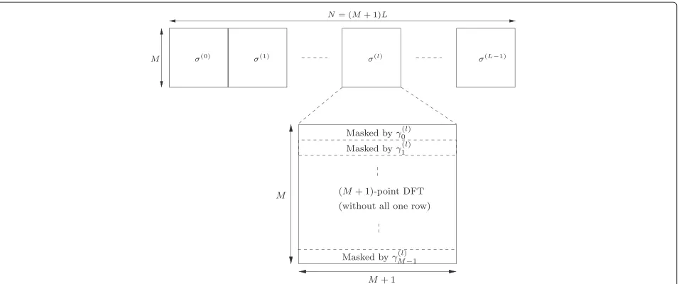
ing matrixAis a concatenation of the L submatrices i.e., A=σ(0)|σ(1)| · · · |σ(L−1). In particular, if L=M−1, thenA=A=σ(0)|σ(1)| · · · |σ(M−2).
Figure 1 illustrates the structure of our new sensing matrixAin Construction 1.
3.2 Implementation
In Construction 1, generating the row index setD effi-ciently is a key issue in implementing the determinis-tic sensing matrix A. InD, as α(pr+1)ev = Tr2r
r (αv) is an element of a pr-ary m-sequence of period p2r − 1 [21], we can compute it by a 2-stage LFSR. Therefore,
each element of D in Equation 1 can be generated by
LFSR, log operation and other basic arithmetics over finite fields.
As the computation over finite fields is not trivial, we introduce an alternative method to generate the indices
of D more efficiently. In the method, we use
cyclo-tomic cosets modulopr+1 andp2r −1 overp, respec-tively, which are always valid for any prime p, since gcd(p,pr+1) =gcd(p,p2r−1)= 1. In what follows, we describe the procedure, where the proof will be given in the Appendix.
Procedure 1.
Figure 1Concatenated structure of new sensing matrixA.It illustrates the concatenated structure of the new sensing matrixAin Construction 1.
by2(2r+1)\ {0} = {u1,. . .,uδ}. Ifp>2, on the other hand, identify a set of coset leaders without
pr+1
2 byp(pr+1)\ { pr+1
2 } = {u1,. . .,uδ}. Note that
u1=0ifp>2.
2. For eachui,1≤i≤δ, compute a positive integer
zi∈Zp2r−1such that
αzi=1+α(pr−1)ui (8)
whereαis a primitive element inFp2r.
3. For eachzi,1≤i≤δ, generate a cyclotomic coset
modulop2r−1overp containingziby
Csi = {zi,zip,. . .,zip
nsi−1}, wheren
siis the smallest positive integer such thatzi≡zipnsi (modp2r−1).
Note that the coset leadersiis not necessarily equal
tozi.
4. Ifp=2,
D=
1≤i≤δ Csi,
and ifp>2,
D=
1≤i≤δ Csi+
M+1
2
where the addition is performed to each element of
1≤i≤δCsi, and computed modulop2r−1. From Remark 2, the index setD should be sorted such that the entries are in decreasing order when computed
moduloM+1, i.e.,D
(modM+1)≡ {M,M−1,. . ., 1}.
Example 3. Letp= 2 andr= 3. Also, letαbe a prim-itive element in F26 satisfying α6+ α +1 = 0. Then,
Procedure 1 generatesM = pr = 8 indices ofDfor our
new sensing matrix:
1. From all cyclotomic cosets modulo 9 overp=2, we identify nonzero coset leaders2(9)\ {0} = {1, 3},
where the cosets areC1= {1, 2, 4, 8, 7, 5}and C3= {3, 6}, respectively.
2. Fromu1=1, Equation 8 yieldsαz1 =1+α7=α26,
wherez1=26. Also, fromu2=3, we have
αz2 =1+α21=α42andz2=42.
3. By successively multiplyingz1=26by 2, we obtain
its cyclotomic cosetC13= {26, 52, 41, 19, 38, 13},
where the coset leader iss1=13. Note that the
multiplication is computed modulop2r−1=63. Similarly, we haveC21= {42, 21}fromz2=42,
wheres2=21.
4. Finally, the index setD is given by
D= {d0,d1,. . .,d7} =C13
C21
= {26, 52, 42, 41, 13, 21, 38, 19}
where we have sorted the indices such that they are in decreasing order when computed modulo 9, i.e.,D (mod 9)≡ {8, 7, 6, 5, 4, 3, 2, 1}.
In practice, we can precomputez1,z2,. . .,zδat items 1 and 2 of Procedure 1 and save them in memory to avoid the algebraic computation of Equation 8 in the hardware. Then,M= pr indices can be generated by items 3 and 4 of Procedure 1. In Example 3, for instance,z1 = 26 and
z2 = 42 can be precomputed. Then, only the two
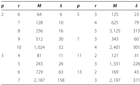
ele-ments need to be stored in the memory to generate eight row indices. Table 2 presentsδor the number ofzis to be stored in the memory for variousM=pr. While a random partial Fourier matrix needs to saveMindices, a storage space forδ ( M)elements is sufficient for our new sens-ing matrix. In conclusion, constructsens-ing our new senssens-ing matrix requires a storage forδelements and an additional circuit for successive multiplication, addition and sorting, which may present a practical benefit over random partial Fourier matrices.
3.3 Theoretical recovery performance
In this subsection, we discuss the geometric properties and the theoretical recovery guarantee of our new sensing matrixA.
Lemma 2.The M×N sensing matrix Ain
Construc-tion 1 has the following properties.
1. The coherence is upper bounded by1/√M. 2. Aforms a tight frame.
3. All the row sums are equal to zero.
Proof. Recall thatA is obtained by row/column rear-rangement ofA. Since the coherence of a matrix does not
change by row/column permutation, the coherence ofA
is also 1/√Mfrom Proposition 1. Note that whenp>2, we have added the constantM+21to each entry of the orig-inalDin Equation 1, which does not change the coherence [19] either. As Ais a set of selected columns ofA, the trices, which shows that item 2 is true. Finally, Equation 5 ensures that no submatrixσ(l)has all one row masked by a constant factor, which concludes that all the row sums of each submatrix are equal to zero, due to the DFT-based structure. Consequently, item 3 is true from the concatenation.
The geometric properties of Lemma 2 meet the
suf-ficient conditions for the new matrix A to achieve
the uniqueness-guaranteed statistical restricted isometry property (UStRIP)[5]. See [27] for the proof of the UStRIP ofA.
With a deterministic sensing matrix of coherence μ,
one can successfully recoverevery s-sparse signal from its measurement as long ass = O(μ−1)[24], which guaran-tees unique recovery of sparse signals with sparsity up to O(√M) by our new sensing matrixA. In an attempt to overcome the theoretical bottleneck, the authors of [28]
discussed the averageperformance of compressed
sens-ing under ageneric s-sparse model, where the positions of nonzero entries of ans-sparse signal are distributed uni-formly at random and their signs are independent and equally likely to be−1 or+1. In what follows, the average recovery performance ofs-sparse signals with the generic s-sparse model is theoretically guaranteed by the sensing matrixA.
Theorem 1. Consider the M×N sensing matrixAin
Construction 1. Let x ∈ RN be an s-sparse signal with the generic s-sparse model. Then, if s = O
M logN
, it is possible to recover xwith probability 1−N−1 from the
measurementAx.
Proof. From Lemma 2,A is a tight frame with
coher-ence μ = O
. For such a matrix, Theorem 2.2 of [29] presents the average recovery performance that if
s = O
to recover xwith probability 1− N−1 from Ax, which
completes the proof.
4 FFT-based signal measurement and recovery
This section describes measurement and recovery pro-cesses with the deterministic compressed sensing matrix
A in Construction 1. With the DFT-based submatrix
structure, we can make use of the FFT technique in the processes.
4.1 Measurement
The measurement process of compressed sensing is accomplished byy = Ax, wherex = (x0,x1,. . .,xN−1)T
(xbl,xbl+1. . .,xbl+b−1)T be a segment of x of length b,
bxl for each l, which implies that the matrix-vector multiplication σ(l)x
l includes to perform the b -point DFT of each segmentxland then to multiply each DFT output byγk(l). Letxk(l)be theb-point DFT ofxl, i.e.,
equivalent to adding up each DFT outputX(kl)weighted by γk(l)for 0≤l≤L−1. In other words,
For fast implementation, the FFT algorithm can be applied to theLdistinct segments ofxsimultaneously in a parallel fashion.
4.2 Reconstruction
For s-sparse signal recovery, we consider the CoSaMP
algorithm presented in Algorithm 2.1 of [20], which is described in Algorithm 1 of this paper. At each iteration, it forms a signal proxy f and identifies a potential can-didateof the signal support by locating the largest 2s components of the proxy. The algorithm then merges the candidatewith the one from the previous iteration, to create a new support set T. To estimate the target sig-nalxi, it solves a least-squares problem and takes only the largestsentries from the signal approximationz. Finally, it updates the current samplevfor the next iteration.
Algorithm 1:CoSaMP recovery algorithm [20]
x0←0,v←u,z←0,i←0 Initialize
repeat i←i+1
f←AHv Form signal proxy
←supp(f2s) Identify large components
T ←∪supp(xi−1) Merge supports
z|T ←A†Tu Estimate signal by least-squares
xi←zs Take the largestsentries
v←u−Axi Update current samples
until a halting criterion is true
In Algorithm 1, the signal proxy isf=AHv=(f0,f1,. . .,
fN−1)T, where v = (v0,v1,. . .,vM−1)T andAH denotes
the conjugate transpose ofA. Initially,vis a (noisy) mea-surement vectoru. At each iteration, it will be updated byv = u−Axi. Considering the submatrix structure of
σ(l), the matrix-vector multiplicationAHvis performed by the reverse operation of the measurement process, i.e., extracting the weight γk(l) from each measurement and then applying theb-point IDFT. For eachl, 0≤l≤L−1,
where ‘∗’ denotes the complex conjugate. Applying the b-point IDFT tov(l)with normalization then yields a seg-ment offof length b, i.e., fl = (fbl,fbl+1,. . .,fbl+b−1)T,
For fast implementation, the FFT algorithm can be applied to theL distinct demasked versions ofv simultaneously in a parallel fashion. Finally, concatenating theLsegments formsf=(fT0 | · · · |fTL−1)T.
While updating current samples at each iteration, the matrix-vector multiplicationAxiis also performed by the FFT algorithm in a similar manner to the measurement process. One may stop the iterations of the CoSaMP algo-rithm if the norm of updated samples is sufficiently small or the iteration counter reaches a predetermined value.
Table one of [20] claimed that forming a signal proxy dominates the algorithm complexity by the cost of matrix-vector multiplication. Thus, each iteration of the FFT-based CoSaMP recovery algorithm has the complexity of O(L×blogb)≈O(NlogM), which is smaller than that of random partial Fourier matrices.
5 Empirical recovery performance
In this section, we compare our new sensing matrices to chirp sensing [6] and random partial Fourier matrices in terms of empirical recovery performance in noiseless and noisy scenarios. For comparison, we assume that a
ran-dom partial Fourier matrix has the same parametersM
andN = (M+1)Las those of our new sensing matrix.
To obtain it, we made ten trials to select M rows
ran-domly from theN-point IDFT matrix, where the
Through experiments, we measured an s-sparse sig-nalx, where thesnonzero entries are either+1 or−1, and their positions and signs are chosen uniformly at random. For signal reconstruction, the FFT-based CoSaMP algorithm was applied to a total of 2, 000 sample vectors measured by the three sensing matri-ces. In Algorithm 1, the iterations are stopped if either
||v|| < 10−4or the iteration counter reaches the sparsity levels.
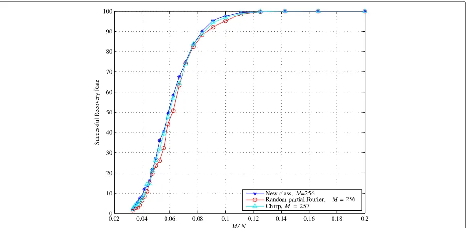
Figure 2 displays successful recovery rates of the three sensing matrices from noiseless measurements at vari-ous compression ratios, where the sparsity level is s =
64. In the figure, for 5 ≤ L ≤ 30, M = 256 and
N = (M+ 1)L for our new sensing and random
par-tial Fourier matrices, while M = 257 andN = MLfor
chirp sensing matrices. With the parameters, each
sens-ing matrix achieves the compression ratios of 0.0333 ≤
M
N ≈ 1L ≤ 0.2. A success is declared in reconstruction if ||x−x||<10−6for the estimatex. The figure shows that
our new sensing matrices have slightly higher recovery rates than the random partial Fourier matrices but have almost the same recovery rates as those of chirp sensing codes.
In noisy compressed sensing, a measured signal is
cor-rupted by additive noise, i.e., u = y + n = Ax+ n,
wherenis the additive white Gaussian noise of zero mean and variance σ2. Then, the input signal-to-noise ratio (SNR) is defined as SNRinput(dB) = 10 log10||
y||2
σ2 . Also,
we define the reconstruction SNR as SNRreconst(dB) = 10 log10||||x−x||x2||2, to measure the recovery performance in
noisy compressed sensing. In the experiments, we fixed
L = 8, whereM=256 and N = L(M+ 1) = 2, 056
for our new sensing and random partial Fourier matrices,
while M=257 and N = ML = 2, 056 for chirp
sens-ing matrices. Figure 3 shows an example of original and reconstructed signals for our new sensing matrix in noisy compressed sensing, where the sparsity level iss=15 and the input SNR is 15 dB.
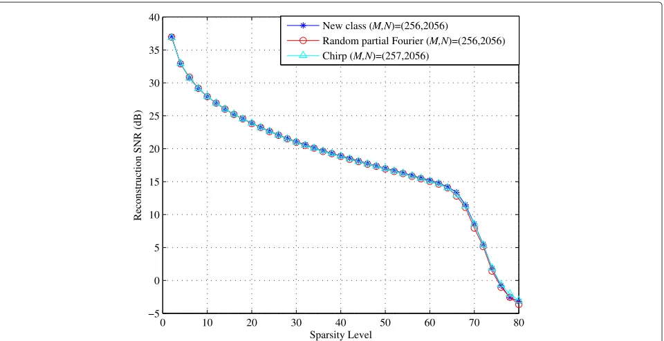
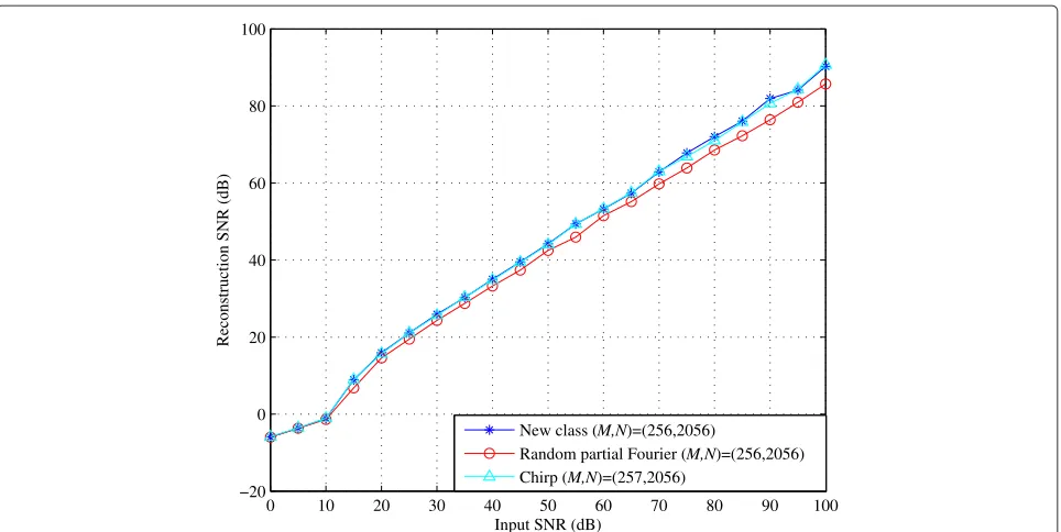
Figure 4 sketches the reconstruction SNR of the three sensing matrices from noisy measurements. In the figure, the input SNR is 15 dB. The figure reveals that our new sensing matrix outperforms the random partial Fourier and the chirp sensing matrices at high sparsity levels, but the differences are negligible. Figure 5 demonstrates reconstruction SNR versus input SNR of the three matri-ces in noisy compressed sensing, where the sparsity level of an original signal is 70. At the sparsity level, we observed that the relationship between reconstruction and input SNR is linear for medium and high input SNR. Our new sensing matrix slightly outperforms the random partial Fourier matrix for high input SNR but shows almost the same trend with the chirp sensing code.
In addition to the above experiments, we attempted an elementary image reconstruction employing the Haar wavelet transform. An original sparsified image was
0.020 0.04 0.06 0.08 0.1 0.12 0.14 0.16 0.18 0.2 10
20 30 40 50 60 70 80 90 100
M/ N
Successful Recovery Rate
New class, M=256
Random partial Fourier, M= 256 Chirp,M= 257
0 200 400 600 800 1000 1200 1400 1600 1800 2000 −1.5
−1 −0.5 0 0.5 1 1.5
Original signal Reconstructed signal
Figure 3An example of original and reconstructed signals for our new sensing matrix in noisy compressed sensing.The figure shows an example of original (white circle) and reconstructed (asterisks) signals of lengthN=2, 056 from its noisy measurement of lengthM=256 for our new sensing matrix, wheres=15 and SNRinput=15 dB.
measured by the three sensing matrices and then recon-structed by the CoSaMP algorithm. We observed that the successfully reconstructed images from three differ-ent matrices are hard to distinguish, and show almost the same reconstruction SNR.
In conclusion, our new sensing matrix showed empiri-cally reliable recovery performance by the CoSaMP algo-rithm in both noiseless and noisy scenarios, which is comparable to those of chirp sensing and random partial Fourier matrices.
0 10 20 30 40 50 60 70 80
−5 0 5 10 15 20 25 30 35 40
Reconstruction SNR (dB)
Sparsity Level
New class (M,N)=(256,2056)
Random partial Fourier (M,N)=(256,2056) Chirp (M,N)=(257,2056)
0 10 20 30 40 50 60 70 80 90 100 −20
0 20 40 60 80 100
Input SNR (dB)
Reconstruction SNR (dB)
New class (M,N)=(256,2056)
Random partial Fourier (M,N)=(256,2056) Chirp (M,N)=(257,2056)
Figure 5Reconstruction SNR versus input SNR in noisy compressed sensing for 70-sparse input signals.The figure displays reconstruction SNR versus input SNR of our new class (asterisks), random partial Fourier (white circle), and chirp sensing (white triangle) matrices in noisy compressed sensing for 70-sparse input signals, whereM=256 andN=2, 056 for our new sensing and random partial Fourier matrices, while
M=257 andN=2, 056 for chirp sensing codes.
6 Conclusions
This paper has constructed a new class of Fourier-based compressed sensing matrices using an almost difference set. We showed that a basic partial Fourier matrix, equiv-alent to the near-optimal partial Fourier codebook pre-sented in [19], could be reprepre-sented as a concatenation of DFT-based submatrices under row/column rearrange-ment. Choosing a full or a part of columns of the con-catenated matrix, we then constructed a new sensing matrix which turns out to be an incoherent tight frame. The new sensing matrix guarantees unique sparse recon-struction with high probability for sparse signals with uniformly distributed supports. Moreover, experimen-tal results revealed that our deterministic compressed sensing guarantees the empirically reliable recovery performance.
In conclusion, compared to existing chirp sensing and random partial Fourier matrices, our new sensing matri-ces have the benefits summarized:
1. Our new deterministic sensing matrices support various parameters ofM=prandN=(M+1)Lfor
any primep and positive integers r and L,
2≤L≤M−1. They are incoherent tight frames for any suchM and N. Compared to chirp sensing codes whereM is generally restricted to a prime number, the new matrices therefore provide more options for the parametersM and N, permitting various
compression ratios ofMN ≈ 1L. A large number of new sensing matrices with a variety of admissible
parameters may have many potential applications in compressed sensing.
2. The deterministic row index structure requires much less storage space than random partial Fourier matrices. Moreover, while theN -point FFT is required for random partial Fourier matrices, the DFT-based submatrix structure of our new sensing matrices allows the(M+1)-point FFT processing, which enables efficient signal measurement and reconstruction with low complexity and fast processing. The benefits in implementation indicate the potential of our new sensing matrices in practical compressed sensing.
Appendix
Proof of procedure 1
First of all, Lemma 3 shows that the indices of D in
Equation 1 are equivalently generated by cyclotomic cosets. In the proof, we use the well-known property that (x+y)pk =xpk+ypk forx,y∈Fpm and any integersm,k.
Lemma 3. Consider all cyclotomic cosets modulo pr+1 over p. From Procedure 1, recall that if p = 2, 2(2r + 1) \ {0} = {u1,. . .,uδ}, and if p > 2, p(pr + 1) \ {pr+1
the cyclotomic coset having the coset leader ui. Also, let
4. Finally, the index setDof Equation 1 is given by
D=
element of the cyclotomic coset containing it. Therefore,1≤i≤δCui=Zpr+1\ {p
r+1
2 } =Iis also
clear.
2. For givenui, the solutionzi∈Zp2r−1of Equation 8 is unique from the structure of the finite fieldFp2r. From the uniqueness,zi=zjif and only ifui=ujfor the smallest positive integer satisfying Equation 11. Similarly,1+α(pr−1)uipnsi =1+α(pr−1)uipnsi = αzipnsi =αzi=1+α(pr−1)ui. Then,
ui≡uipnsi (modpr+1). (13)
From Equations 10 and 13,nuidividesnsisincenuiis the smallest positive integer satisfying Equation 10. Asnsiandnuidivide each other, it meansnui=nsi, solution of Equation 15. For each element
v∈I=1≤i≤δCui, therefore, we conclude that the corresponding solutiondkof Equation 14 constitutes δcyclotomic cosets ofCs1,. . .,Csδeach of which is associated withCu1,. . .,Cuδ, respectively, which yields Equation 9. From item 2,Cs1,. . .,Csδare disjoint, and the setD of Equation 9 hasprdistinct
elements since
|D| =δi=1|Csi| = δ
i=1|Cui| = |I| =p
r.
From Lemma 3, ifp = 2, Equation 9 directly presents
the indices ofDin Equation 2. Ifp>2, on the other hand, we can simply addM+21to each element of Equation 9, to obtain the indices of Din Equation 3. This verifies that Procedure 1 equivalently generates the row index set for our new sensing matrix.
Competing interests
The authors declare that they have no competing interests.
Acknowledgements
This work was supported by the Natural Sciences and Engineering Research Council (NSERC) of Canada.
Received: 26 April 2013 Accepted: 27 September 2013 Published: 5 October 2013
References
1. DL Donoho, Compressed sensing. IEEE Trans. Inf. Theory52(4), 1289–1306 (2006)
2. EJ Candes, J Romberg, T Tao, Robust uncertainty principles: Exact signal reconstruction from highly incomplete frequency information. IEEE Trans. Inf. Theory52(2), 489–509 (2006)
3. EJ Candes, T Tao, Near-optimal signal recovery from random projections: Universal encoding strategies. IEEE Trans. Inf. Theory52(12), 5406–5425 (2006)
4. H Rauhut, Compressive sensing and structured random matrices, in
Theoretical Foundations and Numerical Methods for Sparse Recovery, Radon Series. ed. by M. Fornasier. Computational and Applied Mathematics vol. 9 (deGruyter, Berlin, 2010), pp. 1–92
5. R Calderbank, S Howard, S Jafarpour, Construction of a large class of deterministic sensing matrices that satisfy a statistical isometry property. IEEE J. Sel. Topics Sig. Proc.4(2), 358–374 (2010)
6. L Applebaum, SD Howard, S Searle, R Calderbank, Chirp sensing codes: Deterministic compressed sensing measurements for fast recovery. Appl. Comput. Harmon. Anal.26, 283–290 (2009)
8. T Strohmer, R Heath, Grassmanian frames with applications to coding communication. Appl. Comput. Harmon. Anal.14(3), 257–275 (2003) 9. R Calderbank, S Howard, S Jafarpour, A sublinear algorithm for sparse reconstruction withl2/l2recovery guarantees. 3rd IEEE International
Workshop on Computational Advances in Multi-Sensor Adaptive Processing (CAMSAP), Aruba, 13–16 Dec 2009 (IEEE, Piscataway, 2009), pp. 209–212
10. S Howard, R Calderbank, S Searle, A fast reconstruction algorithm for deterministic compressive sensing using second order Reed-Muller codes. Conference on Information Systems and Sciences (CISS), Princeton, 19–21 March 2008 (IEEE, Piscataway, 2008), pp. 11–15 11. A Amini, V Montazerhodjat, F Marvasti, Matrices with small coherence
using p-ary block codes. IEEE Trans. Sig. Proc.60, 172–181 (2012) 12. RA DeVore, Deterministic constructions of compressed sensing matrices.
J. Complexity.23, 918–925 (2007)
13. S Gurevich, R Hadani, N Sochen, On some deterministic dictionaries supporting sparsity. J. Fourier Anal. Appl.14(5), 859–876
14. Z Xu, Deterministic sampling of sparse trigonometric polynomials. J. Complexity.27, 133–140 (2011)
15. NY Yu, Additive character sequences with small alphabets for compressed sensing matrices. IEEE International Conference on Acoustics, Speech and Signal Processing (ICASSP), Prague, 22–27 May 2011 (IEEE, Piscataway, 2011), pp. 2932–2935
16. S Li, F Gao, G Ge, S Zhang, Deterministic construction of compressed sensing matrices via algebraic curves. IEEE Trans. Inf. Theory.58(8), 5035–5041 (2012)
17. M Mishali, YC Eldar, Blind multiband signal reconstruction: Compressed sensing for analog signals. IEEE Trans. Sig. Proc.57(3), 993–1009 (2009) 18. ME Dominguez-Jimenez, N Gonzalez-Prelcic, G Vazquez-Vilar, R
Lopez-Valcarce, Design of universal multicoset sampling patterns for compressed sensing of multiband sparse signals. IEEE International Conference on Acoustics, Speech and Signal Processing (ICASSP), Kyoto, 25-30 March 2012 (IEEE, Piscataway, 2012), pp. 3337–3340
19. NY Yu, K Feng, A Zhang, A new class of near-optimal partial Fourier codebooks from an almost difference set. Des. Codes Cryptogr (2012). 10.1007/s10623-012-9753-8
20. D Needell, JA Tropp, CoSaMP: Iterative signal recovery from incomplete and inaccurate samples. Appl. Comput. Harmon. Anal.26, 301–321 (2009) 21. SW Golomb, G Gong,Signal Design for Good Correlation - for Wireless
Communication, Cryptography and Radar.(Cambridge University Press, Cambridge, 2005)
22. FJ MacWilliams, NJ Sloane,The Theory of Error-Correcting Codes
(North-Holland, Amsterdam, 1977)
23. KT Arasu, C Ding, T Helleseth, PV Kumar, H Martinsen, Almost difference sets and their sequences with optimal autocorrelation. IEEE Trans. Inf. Theory47(7), 2934–2943 (2001)
24. DL Donoho, M Elad, Optimally sparse representation in general (nonorthogonal) dictionaries vial1minimization. Proc. Natl. Acad. Sci.
100, 2197–2202 (2003)
25. LR Welch, Lower bounds on the maximum cross correlation of the signals. IEEE Trans. Inf. TheoryIT-20, 397–399 (1974)
26. J Kovacevi´c, A Chebira,An Introduction to Frames: Foundations and Trends in Signal Processing, vol. 2. (now Publishers, Hannover, 2008)
27. NY Yu, On statistical restricted isometry property of a new class of deterministic partial Fourier compressed sensing matrices. International Symposium on Information Theory and its Applications (ISITA), Honolulu, 28–31 Oct 2012 (IEEE, Piscataway, 2012), pp. 287–291
28. E Candes, Y Plan, Near-ideal model selection byl1minimization. Ann. Stat.
37(5A), 2145–2177 (2009)
29. S Jafapour, MF Duarte, R Calderbank, Beyond worst-case reconstruction in deterministic compressed sensing. IEEE International Symposium on Information Theory Proceedings (ISIT), Cambridge, 1–6 July 2012 (IEEE, Piscataway, 2012), pp. 1862–1866
30. K Ni, S Datta, P Mahanti, S Roudenko, D Cochran, Efficient deterministic compressed sensing for images with chirps and Reed-Muller codes. SIAM J. Imaging Sci.4(3), 931–953 (2011)
doi:10.1186/1687-6180-2013-155
Cite this article as:Yu and Li:Deterministic construction of Fourier-based compressed sensing matrices using an almost difference set.EURASIP Jour-nal on Advances in SigJour-nal Processing20132013:155.
Submit your manuscript to a
journal and benefi t from:
7Convenient online submission 7Rigorous peer review
7Immediate publication on acceptance 7Open access: articles freely available online 7High visibility within the fi eld
7Retaining the copyright to your article