Combined Emission Dispatch and Economic Dispatch of Power System Including Renewable Sources

Combined Emission Dispatch and Economic

Dispatch of Power System Including

Renewable Sources

Dongara Ganesh Kumar , Dr.P.Umapathi Reddy

Pursuing M.Tech. Department of EEE, SVEC, Tirupati, India

Professor, Department of EEE, SVEC, Tirupati, India

ABSTRACT: The harmful ecological effect by the emission of gaseous polluted from fossil fuel power plants can be reduced by proper load allocation among various generating units of the plant, but this load allocation may lead to increase operating cost of generating units and non-commensurable fuel cost.Various types of economic dispatch in power systems such as multi area economic dispatch with tie line limits, economic dispatch with multiple fuel options, combined economic and emission dispatch problem.This Combined Economic Dispatch and Emission Dispatch problem is a Multi objective problem. This Multi objective problem can be converted in to single objective problem by using penalty factor. This project presents Combined Economic Dispatch Models developed a system consists of multiple photovoltaic plants and thermal units. Reliable and inexpensive electricity provision is one of the significant objective have been developed in order to address the challenge of continuous and sustainable electricity provision at optimized cost. Problem formulated was implemented on two test cases and results obtained from lambda-iteration, as conventional technique and proposed technique results are compared in terms of Cost, Emission, Convergence and No of iterations.

KEYWORDS: Economic Dispatch, Renewable energy, Solar PV generation, Penalty factor.

I INTRODUCTION AND RELATED WORK

An important research has been show up around the world for expansion of continuous, renewable and efficient energy structure in order to meet the requirements of increased population and to reduce the expanded the use of fossil fuels. Expanding energy prices, environmental concerns and expeditious depletion of the known fuel reserves have significantly increased the extension of renewable energy resources. The power sector of Pakistan is designed as an interconnected system and heavily relies on typical sources of generation. This system needs adjustments and improvement in order to meet the twenty first century specifications. Pakistan’s energy incorporate span of almost 67% thermal and 30% hydel resources. According to Pakistan’s energy year book 2012 [1], total generated electrical energy in Pakistan during 2010–2011 was 95,365 GW hand part of different sources is: thermal power 64.3%; hydel29.9% and nuclear and imported 5.8%. In thermal power, oil include the largest part of 35.2% followed by natural gas 29.0% and coal0.1%. On the other hand, the country has a large hidden of solar energy which has been predicted to be everywhere of 2900 GW in [2]. In [3], the author explain the energy scheme of Pakistan and reviewed conventional and Renewable Energy (RE) resources of the county in detail. The author has been exhibited the supply, generation and using of available resources in significant manner. The paper is focused on RE advancement projects in the country, recent progress, planning and public sector goals in this field. Onaverage, solar global insolation of 5–7 kW h/m2/day in almost95% areas of Pakistan with persistence factor of over 85% has been reported in [4,5]. Economic Dispatch (ED) is a significant and most constant step inpower system operational planning [6]. ED is a development complication that set aside power to each committed generating unitso as to underestimate the total operational cost, subject to constraints. Different constraints build power balance, power limits ofgenerators, prohibited operating zones, ramp rate limits etc. Several optimization capacities with equality and non-equalityconstraints have been used for ED and reported inliterature [7].

complete better conclusions [8]. In those days analog computers were used for computational achievement. First computer for transmission loss penalty factor was built up in 1954. By 1955 electronic prong commentator was developed. Digital computers were used for ED first time ever in 1954 and are being used till date [9]. The authors in [10] have approach the capacity of ED used during 1977–1988; optimal power flow, dynamic dispatch, ED in relation to Automatic Generation Control (AGC) and ED with non-conventional sources has been evaluated. Power system subsist of thermal generators has been broadly used to evaluate ED problem. Input–output (consultation productivity) cost curves of thermal generating units are mandatory for ED. The input–output price-tag curve of a thermal generating unit is achieved by multiplying cost per unit heat and its input–output (consultation productivity) heat rate curve[11]. In present days multi-valve steam turbines and multiple fuel turbines are regularly used in generating units.

The ED with piecewise quadratic cost function (EDPQ) and ED with restricted operating zones (EDPO) are the two non-convexED problems [12]. Valve point effects producing a ripple like no convex input–output heat rate curve. Complex constrained ED is forwarded by intelligent methods including Genetic Algorithm (GA), PSO [13,14], Neural Network (NN), Evolutionary Programming(EP), Tabu search etc. [15–17]. Kennedy and Eberhart introducedPSO in 1995 [18]. In this method, movement of particles is dependent on local and social components of velocity. Moreover, maximum value of velocity, Vmax, is also an important parameter. Its low value results in local exploitation while a higher value results in global international analysis. To obtain a better control over local exploitation and global research, an inertia factor x is introduced in[19]. ED with both cost and emission minimization becomes multiobjectiveoptimization problem and is named as Combined Emission Economic Dispatch (CEED). Using PSO, CEED has been solved by Selvakumar et al. [20]. Zhao et al. [21] solved bid based ED using Constriction Factor PSO (CFPSO) and inertia weight. In [22], a hybrid PSO, a combination of PSO and Sub sequent Quadratic Programming (SQP), is introduced in order to solve a non-convex constrainedED problem with valve point effects. In [23], CEED has been solved using a novel PSO scheme taking into account the generator limits and power balance constraints. An improved PSO has been proposed to solve ED problem of hydro-thermal co-ordination in[24]. Authors in [25]have expected scheduled an added to PSO(EPSO) for hydro-thermal scheduling problem which takes into account discrete constraints such as power balance, hydro and thermal generation limit, reservoir storage volume, initial and terminal storage limit, water balance equation and hydro discharge limit. In[26], PSO has been used to evaluate CEED problem with equality constraints handled by different manner and multi-objective optimization problem transformed into a single objective one.

A lot of research on Economic Dispatch (ED) problem has been carried out during last five years. A few instances are as follows. In[8], a non-convex ED problem has been addressed by various hybrid development methods. The problem has been addressed first by developing an extensible and flexible soft computationalframework called ‘‘PED Frame’’, used as a platform for the computer application of different algorithms under scrutiny. This framework has been used to implementGenetic Algorithm (GA) based models and Hybrid models for ED. In [27], a PSO based technique with constriction factor (CFPSO) has been proposed for ED with valve point effects; CFPSO technique proved to be fast converging. In [28], amulti-objective CEED solution has been proposed by using Artificial Bee Colony (ABC) algorithm. For the solution of the problem, multiobjectiveCEED has been converted into single-objective CEED byusing penalty factor. In [29], iteration PSO with time varying acceleration coefficients (IPSO-TVAC) has been proposed for ED with valve-point effects; Iteration term in velocity equation and time varying acceleration coefficients improved the achievement (searching ability) of PSO technique. In [30], a novel optimization methodology has been proposed to solve a large scale non-convexED problem. The proposed approach is based on a hybrid Shuffled Differential progression (SDE) algorithm that combined the benefits of shuffled frog leaping algorithm and differential evolution. The proposed algorithm integrated a new differential mutation operator in order to address the problem of ED.

Dispatch (SCEED) andDynamic Combined Emission Economic Dispatch (DCEED) have been considered. SCEED is performed for full solar radiation level as well as for reduced emission level due to clouds effect whereasDCEED for full radiation only. PSO is used for optimization of the problem and simulation results have been computed in MATLAB. The proposed model contains various different solar plants unlike the workdiscussed in [31, 32]. Power demand data has been obtained from Islamabad Electric Supply Company (IESCO) [34].

II PROBLEM FORMULATION

This area is enthusiastic for question formulation of CEED for apower system having thermal and solar PV generations. As specified earlier, an ED problem can be formulated either statically or dynamically. The mathematical formulation for both cases is worked out in the following subsections.

(a) Mathematical formulation of SCEED with solar power

CEED is a multi-objective optimization problem subsist ofboth economic and environmental dispatch. The CEED problem can be formulated as:

𝑚𝑖𝑛𝐺= 𝑛𝑖=1(𝐹𝑡 𝑃𝑡 + 𝐸𝑡 𝑃𝑡 (1)

Where G is objective function to be minimized, Fi(Pi) represents fuel cost and Ei(Pi) denotes the emissions of ith generating unit. This function is to be minimized subject to following constraints.

Equality constraint:

𝑝𝑖 𝑛

𝑖=1 − 𝑃𝐿− 𝑃𝑑 = 0 (2)

Where Pi is power generated by ith unit, PL represents power loss, Pdis power demand and n is the total number of generating units.

Inequality constraint:

𝑝𝑚𝑖𝑛 ≤ 𝑝𝑖 ≤ 𝑝𝑖𝑚𝑎𝑥(3)

WherePiminandPimax are the minimum and maximum power limits ofith generating unit, respectively.

𝐹𝑖 𝑝𝑖 = 𝑎𝑖𝑝𝑖2+ 𝑏𝑖𝑝𝑖 + 𝑐𝑖+ 𝑒1∗ sin⁡(𝑓1∗ 𝑝𝑚𝑖𝑛 − 𝑝𝑖 ) 𝑠 𝑕(4)

Fi(Pi), Ei(Pi) in Eq. (1) and PL in Eq. (2) can be formulated as follows[35].

𝐸𝑖 𝑝𝑖 = 𝛼𝑖𝑝𝑖2+ 𝛽𝑖𝑝𝑖+ 𝛾𝑖 + 𝜖𝑖⁡∗ 𝑒𝑥𝑝 𝛿𝑖− 𝑝𝑖 ) 𝑘𝑔_𝑕(5)

Where ai, bi, ci, ei and fi are fuel cost coefficients of ithgenerating unit.

𝐸𝑖 𝑝𝑖 = 𝛼𝑖𝑝𝑖2+ 𝛽𝑖𝑝𝑖+ 𝛾𝑖 + 𝜖𝑖⁡∗ 𝑒𝑥𝑝 𝛿𝑖∗ 𝑝𝑖 ) 𝑘𝑔 _𝑕(6)

Where /i, bi, ci, ei and di are emission coefficients of ithgenerating unit. Power losses can be calculated using the equation:

𝑃𝐿= 𝑛𝑖=1 𝑛𝑗 =1𝑝𝑖𝐵𝑖𝑗𝑝𝐽 (7)

Where B is loss coefficient matrix.

By introducing a price penalty factor ‘h’, the multi-objective optimization function presented by Eq. (1)can be converted into single objective optimization function. Therefore, by substituting and Ei from Eqs.(4) and (5) respectively and introducing ‘h’ inEq. (1), the CEED objective function can be defined as [28]:

𝑕𝑖(𝛼𝑖𝑝𝑖2+ 𝛽𝑖𝑝𝑖 + 𝛾𝑖 + 𝜖𝑖⁡∗ 𝑒𝑥𝑝 𝛿𝑖∗ 𝑝𝑖 ) 𝑆 𝑕(8)

Where hi is given as:

𝑕𝑖=

𝑎𝑖𝑝𝑖2+𝑏𝑖𝑝𝑖+𝑐𝑖+ 𝑒1∗sin ⁡(𝑓1∗ 𝑝𝑚𝑖𝑛−𝑝𝑖 )

(𝛼_𝑖𝑝_𝑖2+𝛽_𝑖𝑝_𝑖+𝛾𝑖 + 𝜖_𝑖⁡∗𝑒𝑥𝑝 𝛿_𝑖∗𝑝_𝑖 ) (9)

The power generated by a solar plant can be represented as [31]:

𝑝𝑔𝑠 = 𝑝𝑟𝑎𝑡𝑒𝑑 1 + 𝑇𝑟𝑒𝑓 − 𝑇𝑎𝑚𝑏 × 𝛼 × 𝑆_𝑖 1000(10)

Where Prated is its rated power, Trefis the reference temperature, Tambis the ambient temperature, α is temperature coefficient, Si isthe incident solar radiation. With m solar plants taking part in the dispatch, the solar share (the scheduled solar power) is given as:

Solar share = 𝑚𝑖=1𝑝𝑔𝑠𝑗× 𝑢𝑠𝑗 (11)

WherePgsj is power available from jth solar plant and Us denotes status of jth solar plant which is either 1 (ON) or 0 (OFF).The cost of solar power is represented as follows.

Solar cost= 𝑚𝑗 =1𝑝𝑢𝑐𝑜𝑠𝑡𝑗× 𝑝𝑔𝑠𝑗 × 𝑢𝑠𝑗(12)

WherePUCostj is per unit cost of jth solar plant. Along with cost minimization, another objective is to minimize the difference between the total available solar power and the solar share in plan to achieve the property benefit of solar availability. Therefore, with solar generation included in the dispatch, the objective function in Eq. (7) becomes:

Min𝐹𝑅= 𝑛𝑖=1𝑎𝑖𝑝𝑖2+ 𝑏𝑖𝑝𝑖+ 𝑐𝑖+ 𝑒1∗ sin 𝑓1∗ 𝑝𝑚𝑖𝑛 − 𝑝𝑖 +𝑕𝑖(𝛼𝑖𝑝𝑖2+ 𝛽𝑖𝑝𝑖+ 𝛾𝑖 + 𝜖𝑖⁡∗ 𝑒𝑥𝑝 𝛿𝑖∗ 𝑝𝑖 ) +

𝑝𝑢𝑐𝑜𝑠𝑡𝑗× 𝑝𝑔𝑠𝑗× 𝑢𝑠𝑗 𝑚

𝑗 =1 𝑘𝑠( 𝑚𝑗 =1𝑝𝑔𝑠𝑗− 𝑚𝑗 =1𝑝𝑔𝑠𝑗× 𝑈𝑆𝐽 (13)

Subject to

𝑝𝑑 + 𝑝𝑙− 𝑛𝑖=1𝑝𝑖− 𝑚𝑗 =1𝑝𝑔𝑠𝑖× 𝑢𝑠𝑗 = 0 (14)

𝑝𝑚𝑖𝑛 ≤ 𝑝𝑖 ≤ 𝑝𝑖𝑚𝑎𝑥(15)

Where Ks is a constant used to make the last term of Eq. (12) compatible with the other terms. Moreover this allows us to control the relative importance of the difference term compared to other terms.

(b) Mathematical formulation of dynamic CEED with solar power

DCEED is a further constructive case in which it is aimed to give appropriate powers to generating units for minimum cost of procedure ina organizing horizon over twenty-four hours a day. The ramp rate limits are treated in this problem. In case of DCEED problem, the mathematical formulation in Eq. (12) becomes:

Min𝐹𝑅= 𝑁𝑡=1 𝑛𝑖=1(𝑎𝑖𝑝𝑖2+ 𝑏𝑖𝑝𝑖+ 𝑐𝑖+ 𝑒1∗ sin 𝑓1∗ 𝑝𝑚𝑖𝑛 − 𝑝𝑖𝑡 𝑕𝑖(𝛼𝑖𝑝𝑖2+ 𝛽𝑖𝑝𝑖 + 𝛾𝑖 + 𝜖𝑖⁡∗ 𝑒𝑥𝑝 𝛿𝑖∗

𝑝𝑖𝑡)𝑗=1𝑚𝑝𝑔𝑠𝑗𝑡−𝑗=1𝑚𝑝𝑔𝑠𝑗𝑡×𝑈𝑠𝑗𝑡) 𝑗=1𝑚𝑝𝑢𝑐𝑜𝑠𝑡𝑗×𝑝𝑔𝑠𝑗×𝑢𝑠𝑗𝑡𝑘𝑠(𝑗=1𝑚𝑝𝑔𝑠𝑗𝑡−𝑗=1𝑚𝑝𝑔𝑠𝑗𝑡×𝑈𝑠𝑗𝑡)

(16)

The ramp rate limits regulate the range within which the generation of a thermal unit may increase or decrease. The power generation of thermal units is strained by the ramp rate limits as follows:

𝑝𝑖𝑡− 𝑝𝑡𝑡−1≤ 𝑢𝑅𝑖(17)

𝑝

− 𝑝

_{≤ 𝐷𝑅}

𝑖 (18)

max⁡(𝑝𝑖𝑚𝑖𝑛, 𝑈𝑅𝑖− 𝑝𝑖𝑡) ≤ 𝑝𝑖𝑡 ≤ min⁡(𝑝𝑖𝑚𝑎𝑥, 𝑝𝑖𝑡−1− 𝐷𝑅𝑖𝑡 (19)

The power balance constraint for DCEED can be formulated as:

𝑝𝑑𝑡 + 𝑝𝐿𝑡− 𝑃𝑡𝑡− 𝑝𝑔𝑠𝑗𝑡 𝑚 𝑗 =1

× 𝑈𝑆𝐽𝑡 = 0 𝑛

𝑖=1

The share of solar power at any time, based on 30% upper limit[31], is constrained as:

𝑝𝑔𝑠𝑗𝑡 𝑚 𝑗 =1

× 𝑈𝑆𝐽𝑡 ≤ 0.3 × 𝑝𝑑𝑡∀𝑈𝑠𝑗𝑡𝜖 0,1 21

(c ) Optimization method

It is accessible from the above mentioned problem formulation that CEED with solar generation is a Mixed Integer Optimization Problem (MIOP). The decision variables for thermal machines arecontinuous whereas the variables for solar plants are binary. In order to solve this problem, PSO for MIOP is used in this work. The PSO for MIOP is essentially a combination of classical PSOand Binary PSO (BPSO).

(a.1)Classical PSO

PSO is an development and expansion technique inspired by bird flocking. To define PSO we can imagine a block of birds searching for food. This swarm flocks to search the food anyway in a specializedregion. All the birds are supposed to be searching for a single piece of food. At any time during search, each bird has a environment andmomentum. Birds move with familiarity of distance to food but not its exact location. Terrific blue print planned by birds is to follow a bird neighbouring to food. PSO generates use of above mentioned scheme to solve optimization problems. In PSO each bird is well asparticle which is a possible solution in search space. Number of all particles in a search space represents size of swarm (or population). Each particle has a position in search space, velocity and fitness value. Fitness value for a particle is obtained by objective (fitness) function evaluation. Following are the steps of PSO procedure._

 Starts with decision of swarm/population size which is problem specific i.e. it depends on complexity of problem.

 Particles are then initialized randomly for their positions andvalocities. In an N dimensional optimization problem, the position

𝑋

= 𝑥

, 𝑋

, , , , , , , , , 𝑋

of an ith particle is an array of 1 _ N. i.e.,

𝑣

= 𝑣

, 𝑣

, , , , , , , , , 𝑣

 Fitness for each particle is obtained by evaluating the objective function given as:

𝑓

= 𝑓 𝑋

, 𝑋

, , , , , , , , , 𝑋

(24)

 Two best positions pbest and gbest. are selected for next iteration. pbest is personal best position obtained by a particles.

gbest is global best position among all pbest. Incase of first iteration, pbest is same as randomly initialized position of a particle while in case of next iterations, it is the position of a particle having best fitness value up to that defenite iteration.

𝑉

= 𝜔

_𝑣

𝑖𝑘

+ 𝑐

𝑟

𝑝𝑏𝑒𝑠𝑡

− 𝑋

+ 𝑐

𝑟

(𝑔𝑏𝑒𝑠𝑡

− 𝑋

WhereVkiisvelocity of ith particle at iteration k. xk is a parameter known as inertia weight at iteration k. C1 and C2 are acceleration coefficients. r1 and r2 are random numbers between (0, 1). pbestkiis best position of ith particle at iteration k. Xkiis position of ithparticle at iteration k. gbestk is global best position at iteration kand Vkþ1i is updated velocity at iteration k + 1. Vkiwhich is the velocity of ith particle at kth iteration should bewithin range of its minimum and maximum values, i.e.,

𝑣𝑚𝑖𝑛 ≤ 𝑣𝑖𝑘≤ 𝑉𝑚𝑎𝑥(26)

Inertia weight, xk, at each iteration is modified using following equation.

𝜔𝑘_{= 𝜔} 𝑚𝑎𝑥 −

𝜔𝑚𝑎𝑥 − 𝜔𝑚𝑖𝑛

𝑖𝑡𝑒𝑟𝑚𝑎𝑥

× 𝑘 (27)

Whereωmax is maximum value of inertia weight. ωminis minimum value of inertia weight. Itermax is maximum number of iterations.

 After having value of updated velocity, position of each particle is updated using following equation.

𝑋

= 𝑋

+ 𝑣

(28)

 Fitness is evaluated for updated position of each particle; pbestand gbest are procedure for next iteration.

 The process is repeated until a convergence criterion is satisfied.

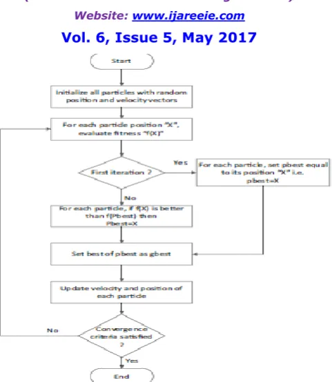
All the above specified steps for PSO agenda are depicted in the flow chart given in Fig. 1.

(a.2) Binary PSO (BPSO)

Binary version of PSO is used to better the complication having binary decision variables i.e. having values either 0 or 1. The steps of BPSO procedure are same as that of real valued PSO except following

Differences: As the variables in BPSO are binary, therefore particles are initialized anyway for their binary positions.

𝑋

= 𝑥

, 𝑋

, , , , , , , , , 𝑋

Each aspect of a particle is assigned a binary value with a probability of 0.5 as following:

𝑋𝑖𝑒 = 𝑓 𝑥 =

Fig. 1. Flow chart of PSO algorithm.

 Position is updated as following:

𝑋𝑖𝑑𝑘+1= 𝑓 𝑥 = 1, 𝑖𝑓 𝑟𝑎𝑛𝑑 < 𝑠𝑖𝑔𝑚𝑜𝑖𝑑(𝑣𝑖𝑘 𝑘 +1₎

0, 𝑜𝑡𝑕𝑒𝑟𝑤𝑖𝑠𝑒 (31)

The elliptical function in above equation, used to scale velocitiesbetween 0 and1, is calculated as:

Sigmoid (

𝑣

) =

1+𝑒−𝑣𝑖𝑑𝑘 +1

(

)

(a.3) PSO for MIOP applied to CEED with solar power

Following are the steps to optimize the SCEED problem (Eqs.(12)–(15)) by means of PSO.

 _Control parameters are selected.

 Initialization of position and velocity for each particle. Each particle contains continuous as well as binary variables.

𝑋

= 𝑃

, 𝑃

, , , , , , , , , 𝑃

𝑢

, 𝑢

, , , , , , , , , 𝑢𝑠

Wherein and UsiD are the power of dth thermal unit and Dthsolar plant in ithparticle. EachPid is initialized randomly using following equation:

𝑃

= 𝐿𝐵 + 𝑟𝑎𝑛𝑑 × 𝑈𝐵 − 𝐿𝐵

LB and UB represent lower bound and upper bound of thermal unitsrespectively. Each UsiD is initialized randomly using Eq. (30).Where D = 1, 2. . . m

 Velocity for each particle is initialized between 0 and 1. Fitness for each particle in Eq. (12)is evaluated and pbest and gbest areselected.

 Fitness in Eq. (12)is evaluated for each updated position, pbestand gbest are obtained for next iteration. The process is repeated until the convergence criterion is satisfied.

III TEST SYSTEM

In this section the proposed model has been implemented ontwo test systems in order to investigate both SCEED and DCEED.

(a)Test system-I

The test system-I add 6 thermal units and 13 solar plantsand is supposed to be operated in Islamabad region of Pakistan. The data for thermal units has been taken from [36] and ispresented in Tables 1 and 2.Table 1 present’s fuel cost coefficients as well as minimum andmaximum power limits whereas Table 2 contains emission.

Coefficients for the preferred machines. The data for solar plants hasbeen presented in Tables 3 and 4.

Table 3 presents power appraisal and per unit costs of different solar plants, approximated to be within the range provided in[37]. Table 4 encompasses global solar radiation as well as temperature and load profiles of Islamabad for the 17th day of July 2012.In this paper, global solar radiation data has been generated using Geospatial Toolkit, data related to power demand of Islamabad region has been taken from IESCO [34] and temperature profile has been taken from [38]. The 17th day of July has been selected arbitrarily from the only available demand data of July, 2012.

(b)Test system-II

The test system-II is also comprised of 6 thermal units and 13solar plants. The data used for solar plants is the same as given in test system-I whereas the data for thermal units and load demand has been taken from [38] and are presented in Tables 5and 6 respectively.

V MATLAB RESULTS

PSO were: C1, C2 = 2; r1, r2 = random numbers between 0 and 1; Maximum number of iterations = 1500; swarm size = 10. Maximum and minimum values of velocity are0.5 ⁄ Pmax and _0.5 ⁄ Pmin respectively. Best results were obtained by setting maximum and minimum values of x to 0.4 and 0.1respectively, as evident from Table 7.The table presents the best values of objective function (Eq.(12)) obtained with various settings of solar plants are considered to be operating for 6 h a day, from10:00 to 16:00 h, as In Pakistan, these hours provide maximum radiation and are free of shadow effects in almost all the seasons. Following are the results and discussions for both cases.

(a) Case I

In this case, the simulations have been carried out for both full and reduced solar radiation; later is the case of cloudy weather. Simulation results of static CEED are depicted in Figs. 2–4 as wellas in Tables 8–13. Graphs in Figs. 2–4 show simulation results in terms of the fitness value (FT) versus iterations. As evident fromFigs. 2–4, the algorithm converges within 1000 iterations.

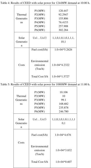
Table 4: Results of CEED with solar power for 1244MW demand at 10:00 h. Thermal Generatio ns P1(MW) P2(MW) P3(MW) P4(MW) P5(MW) P6(MW) 120.447 92.2947 155.806 76.4153 257.908 302.284 Solar Generatio n

Us1…Us13 1,1,0,1,0,1,0,1,1,1, 10,1 Costs Fuel cost($/h) Environmental emission (Ton/h)

Total Cost $/h

1.0+04*5.2626

1.0+04*4.2322

1.0+04*1.5727

Table 5: Results of CEED with solar power for 1088MW demand at 11:00 h.

Thermal Generatio ns P1(MW) P2(MW) P3(MW) P4(MW) P5(MW) P6(MW) 10.106 10 99.1 168.682 235.878 246.780 Solar Generatio n

Us1…Us13 1,1,0,1,0,1,0,1,1,1,1 0,1 Costs Fuel cost($/h) Environmental emission (Ton/h)

Total Cost $/h

1.0+04*4.676

1.0+04*3.832

1.0+04*0.607

Thermal Generati ons P1(MW) P2(MW) P3(MW) P4(MW) P5(MW) P6(MW) 10 10.219 194.931 177.401 224.868 303.564 Solar Generati on

Us1…Us13 1,1,0,1,0,1,0,1,1, 1,10,1 Costs Fuel cost($/h) Environment al emission (Ton/h) Total Cost $/h 1.0+04*4.676 1.0+04*3.832 1.0+04*1.675

Table 7: Results of CEED with solar power for 1135 MW demand at 13:00 h.

Thermal Generatio ns P1(MW) P2(MW) P3(MW) P4(MW) P5(MW) P6(MW) 10.859 118.131 147.927 186.363 150.771 221.081 Solar Generatio n

Us1…Us13 1,1,0,1,0,1,0,1,1,1, 10,1 Costs Fuel cost($/h) Environmental emission (Ton/h)

Total Cost $/h

1.0+04*4.413

1.0+04*3.072

1.0+04*1.531

Thermal Generation

s

P1(MW) P2(MW) P3(MW) P4(MW) P5(MW) P6(MW)

65.283 97.289 250 107.640 252.794 297.757

Solar

Generation Us1…Us13 1,1,0,1,0,1,0,1,1,1,10 ,1

Costs

Fuel cost($/h)

Environmental emission

(Ton/h)

Total Cost $/h

1.0+04*5.508

1.0+04*4.701

1.0+04*1.667

Table 9: Results of CEED with solar power for 1074 MW demand at 15:00 h.

Thermal Generations

P1(MW) P2(MW) P3(MW) P4(MW) P5(MW) P6(MW)

82.760 60.696 249.257 96.2554 182.725 190.648

Solar

Generation Us1…Us13 1,1,0,1,0,1,0,1,1,1 ,10,1

Costs

Fuel cost($/h)

Environmental emission

(Ton/h)

Total Cost $/h

1.0+04*4.505

1.0+04*3.243

Units P1–P6 are well within constraint limits. It can be noted from Tables8–13that the solar power percentage is well within the upper bound. The optimized cost values are consistent with the various shares of thermal and solar power generation. The innovation increases or decreases the solar share based on accessible solar radiation and temperature at any time as obvious from Fig. 5.

The solar share is increased or decreased by turning ON or OFF the applicable solar units. For instance, the number of solar units that are OFF in both Tables 8 and 10 is 4. Turning OFF the solar unit number 1, 3, 8 and 11 at time 10:00 h, as clear from Table 8, results in the solar share of 238.825 MW. On the other hand, Table 10 depict that turning OFF the solar unit number 3, 7, 8 and 12 at time 12:00 h version for the solar share of 319.1076 MW. As the solar share is increased, thermal share gets reduced for a given load demand. Therefore by increasing the solar share, the solar cost is increased whereas fuel cost, emission cost and emissions get reduced; which is evident from Tables 8 and 10 where the load demands are approximately equal, i.e. 1244MW and 1240MWrespectively. In Table 8, the solar cost is 1.0e + 04 ⁄ 6.2322 $/h and the fuel cost, emission cost and emissions are 1.0e + 04 ⁄5.2626 $/h, 1.0e + 04 ⁄ 4.2322 $/h and 1.0e + 03 ⁄ 0.8808 kg/respectively, with solar share of 238.825MW whereas in Table 10,the solar cost is increased to 1.0e + 04 ⁄ 8.2436 $/h while the fuel cost, emission cost and emissions are shortened to 1.0e + 04 ⁄ 4.6762 $/h, 1.0e + 04 ⁄ 3.8326 $/h and 1.0e + 03 ⁄0.8607 kg/h respectively, for increased solar share of 319.1076 MW. The consequence of solar share on total cost is much greater as compared to thermal share because of higher per unit costs of solar generating units. Therefore, the total cost is higher in Table 10 as compared to that in Table 8. This effect can also be seen in Fig. 2, where the fitness value increases from time 10 to12 as the solar share is increased. Complementary relations can be found by analyzing the results in Tables 9 and 13where the load demands are 1088MW and 1074MW respectively. The value of Ks has been experimentally set to 1.0e + 03 which results in maximum solar share of 319.1076MW which is 25.73%of load demand, a value near to the solar share upper bound. By decreasing the value of Ks, the consequence of difference in accessible solar power and the solar share in Eq. (12)gets reduced and vice versa; the resulting solar past varies respectively. Display Fig.5shows the solar share for various levels of solar radiation. The solar radiation often gets reduced due to clouds, depending on various parameters like thickness, height, amount, etc. of clouds. As we have taken into account the global solar radiation which is less afflicted by clouds as difference to beam radiation, therefore Tests have been carried out for estimated reductions of 15% and30%in solar radiation. It is evident from Fig.5that the solar share gets reduced for reduced solar radiation, in an normal manner.

Fig. 5. Solar shares at different solar radiation levels.

Fig.6.Load ramp seen by thermal units at different hours.

VI. CONCLUSIONS

REFERENCES

[1] Pakistan, Hydro carbon development institute of, Pakistan energy yearbook2012. Islamabad: Ministry of petroleum and natural resources Pakistan; 2012.

[2] Mahmood A, Javaid N, Zafar A, Riaz RA, Ahmed S, Razzaq S. Pakistan’s overall energy potential assessment, comparison of TAPI, IPI and LNG gas projects. Renew Sustain Energy Rev 2014;2014(31):182–93.

[3] Sheikh M. Energy and renewable energy scenario of Pakistan.Renew Sustain Energy Rev 2010;14(1):354–63. [4] Shamshad K. Solar insolation over Pakistan. J SES (Taiyo Enerugi)1998;24(6):30.

[5] Sheikh M. Renewable energy resource potential in Pakistan. Renew Sustain Energy Rev 2009;13(9):2696–702.

[6] Morshed MJ, Asgharpour A. Hybrid imperialist competitive-sequential quadratic programming (HIC-SQP) algorithm for solving economic load dispatch with incorporating stochastic wind power: a comparative study on heuristic optimization techniques, techniques.Energy Conver Manage2014;84:30–40. ISSN 0196-8904, vol. 84, No. August 2014, p. 30–40.

[7] Xiong G, Li Y, Chen J, Shi D, Duan X. Polyphyletic migration operator and orthogonal learning aided biogeography-based optimization for dynamiceconomic dispatch with valve-point effects. Energy Convers Manage 2014;80(April):457–68.

[8] Malik TN. Economic dispatch using hybrid approaches.Taxila: University of Engineering & Technology; 2009. [9] Happ H. Optimal power dispatch – A comprehensive survey. Power ApparSystIEEE Trans 1977;96(3):841–54. [10] Chowdhury BH, Rahman S. IEEE Trans 1990;5(4):1248–59.

[11] Wood AJ, Wollenberg BF. Power generation, operation, and control.John Wiley& Sons; 2012.

[12] Lin W-M, Cheng F-S, Tsay M-T. Nonconvex economic dispatch by integrated artificial intelligence.Power Syst IEEE Trans 2001;16(2):307–11. [13] Jeyakumar D, Jayabarathi T, Raghunathan T. Particle swarm optimization forvarious types of economic dispatch problems. Int J Electr Power Energy Syst2006;28(1):36–42.

[14] Selvakumar AI, Thanushkodi K. A new particle swarm optimization solution tononconvex economic dispatch problems.Power Syst IEEE Trans2007;22(1):42–51.

[15] Lee KY, Arthit S-Y, June HP. Adaptive Hopfield neural network for economic.IEEE Trans Power Syst 1998:519–26.

[16] Park Y-M, Jong-Ryul W, Jong-Bae P. A new approach to economic load dispatch based on improved evolutionary programming.EngIntellSyst Elect Eng Commun 6.2 1998:103–10.

[17] Mantawy AH, Soliman SA, El-Hawary ME. A new Tabu search algorithm for thelong term hydro scheduling problem. In: Proceedings of the large engineering systems conference on power engineering; 2002.

[18] Kennedy J. Particle swarm optimization. Encyclopedia Mach Learn2010:760–6.

[19] Shi Y, Eberhart R. A modified particle swarm optimizer. In: Evolutionary computation proceedings, 1998.IEEE world congress on computational intelligence.The 1998 IEEE international conference on, 1998.

[20] Kumar AIS, Dhanushkodi K, JayaKumar J, Paul CKC. Particle swarm optimization solution to emission and economic dispatch problem. In:TENCON 2003. Conference on convergent technologies for the Asia-Pacificregion, 2003.

[21] Bo Z, Yi-jia C. Multiple objective particle swarm optimization technique for economic load dispatch. J Zhejiang UnivSci A 2005;6(5):420–7. [22] Victoire TAA, Jeyakumar AE. Reserve constrained dynamic dispatch of units with valve-point effects.Power Syst IEEE Trans 2005;20(3):1273–82.

[23] Abido M. Multiobjective particle swarm optimization for environmental/economic dispatch problem.Electric Power Systems Res 2009;79(7):1105–13.

[24] Titus S, Jeyakumar AE. Hydrothermal scheduling using an improved particle swarm optimization technique considering prohibited operating zones.IntJournal SoftComput 2007;2(2):313–9.

25] Yuan X, Wang L, Yuan Y. Application of enhanced PSO approach to optimal scheduling of hydro system. Energy Convers Manage 2008;49(11):2966–72.

[26] Alrashidi M, El-Hawary M. Impact of loading conditions on the emissioneconomic dispatch. In: Proceedings of world academy of science: engineering & technology, vol. 41; 2008.

[27] Lim SY, Montakhab M, Nouri H. Economic dispatch of power system using particle swarm optimization with constriction factor. Int J Innovat Energy Syst Power 2009;4(2):29–34.

[28] Sonmez Y. Multi-objective environmental/economic dispatch solution with penalty factor using Artificial Bee Colony algorithm. Sci Res Essays 2011;6(13):2824–31.

[29] Srinivasa Reddy AAVK. Shuffled differential evolution for large scale economic dispatch.Electric Power Syst Res 2013;96:237–45.

[31] Brini S, Abdullah HH, Ouali A. Economic dispatch for power system included wind and solar thermal energy.Leonardo J Sci 2009;14:204–20. [32] ElDesouky A. Security and stochastic economic dispatch of power system including wind and solar resources with environmental consideration. Int J

Renew Energy Res 2013;3(4):951–8.

[33] Jeddi B, Vahidinasab V. A modified harmony search method for environmental/ economic load dispatch of real-world power systems. Energy Convers Manage 2014;78:661–75.

[34] IESCO, Load management curve July, 2012. Islamabad: Islamabad Electric Supply Company; 2012.

[35] Emmanuel DM, Nicodemus AO. Combined economic and emission dispatch solution using ABC_PSO hybrid algorithm with valve point loading effect. Int J Sci Res Publ 2012;2(12):1–9.

[36] Manteaw ED, Odero NA. Multi-objective environmental/economic dispatch solution using ABC_PSO hybrid algorithm.Int J Sci Res Publ 2012;2:12.

BIOGRAPHY

Dongara Ganesh Kumar pursuing M.Tech degree in the stream of Electrical Power Systems from

Sree Vidyanikethan Engineering College (Autonomous), Tiurpati, India. He was completed his B.Tech from SRET (2010-14) in the stream of Electrical and Electronics Engineering.