Solving Hard Lattice Problems and the Security of
Lattice-Based Cryptosystems
Thijs Laarhoven
∗Joop van de Pol
†Benne de Weger
∗September 10, 2012
Abstract
This paper is a tutorial introduction to the present state-of-the-art in the field of security of lattice-based cryptosystems. After a short introduction to lattices, we describe the main hard problems in lattice theory that cryptosystems base their security on, and we present the main methods of attacking these hard problems, based on lattice basis reduction. We show how to find shortest vectors in lattices, which can be used to improve basis reduction algorithms. Finally we give a framework for assessing the security of cryptosystems based on these hard problems.
1
Introduction
Lattice-based cryptography is a quickly expanding field. The last two decades have seen exciting devel-opments, both in using lattices in cryptanalysis and in building public key cryptosystems on hard lattice problems. In the latter category we could mention the systems of Ajtai and Dwork [AD], Goldreich, Goldwasser and Halevi [GGH2], the NTRU cryptosystem [HPS], and systems built on Small Integer Solu-tions [MR1] problems and Learning With Errors [R1] problems. In the last few years these developments culminated in the advent of the first fully homomorphic encryption scheme by Gentry [Ge].
A major issue in this field is to base key length recommendations on a firm understanding of the hardness of the underlying lattice problems. The general feeling among the experts is that the present understanding is not yet on the same level as the understanding of, e.g., factoring or discrete logarithms. So a lot of work on lattices is needed to improve this situation.
This paper aims to present a tutorial introduction to this area. After a brief introduction to lattices and related terminology in Section 2, this paper will cover the following four main topics:
• Section 3: Hard Lattice Problems,
• Section 4: Solving the Approximate Shortest Vector Problem,
• Section 5: Solving the Exact Shortest Vector Problem,
• Section 6: Measuring the Practical Security of Lattice-Based Cryptosystems.
Section 3 on hard lattice problems presents a concise overview of the main hard lattice problems and their interrelations. From this it will become clear that the so-calledApproximate Shortest Vector Problem
is the central one. The paramount techniques for solving these problems are the so-called lattice basis
∗Department of Mathematics and Computer Science, Eindhoven University of Technology, The Netherlands.
reduction methods. In this area a major breakthrough occurred in 1982 with the development of the LLL algorithm [LLL]. An overview of these and later developments will be given in Section 4, with a focus on practical algorithms and their performance. In Section 5, techniques for solving theExact Shortest Vector Problem, such as enumeration and sieving, are discussed. These techniques can be used to find shortest vectors in low dimensions, and to improve lattice basis reduction algorithms in high dimensions. Finally, in Section 6, we look at lattice-based cryptography. Using theoretical and experimental results on the performance of the lattice basis reduction algorithms, we aim to get an understanding of the practical security of lattice-based cryptosystems.
For evaluating the practicality of secure cryptosystems, both security issues and issues of performance and complexity are of paramount importance. This paper is only about the security of lattice based cryptosys-tems. Performance and complexity of such cryptosystems are out of scope for this paper.
2
Lattices
This section gives a brief introduction to lattices, aiming at providing intuition rather than precision. A much more detailed recent account can be found in Nguyen’s paper [N], on which this section is loosely based.
2.1
Lattices
The theory of lattices may be described asdiscrete linear algebra. The prime example for the concept of lattice isZn, the set of points in then-dimensional real linear space
Rnwith all coordinates being integers.
This set forms a group under coordinate-wise addition, and is discrete, meaning that for every point in the set there is an open ball around it that contains no other point of the set. On applying any linear transformation toZnthe additive group structure and the discreteness are preserved. Any such image of Znunder a linear transformation is called alattice. Indeed, any discrete additive subgroup ofRncan be
obtained as a linear transformation ofZn. Therefore in the literature lattices are often defined asdiscrete
additive subgroups of Rn.
In this paper we further restrict to lattices inZn. The linear transformation applied to
Znthat produces the
lattice transforms the standard basis ofZninto a set ofgeneratorsfor the lattice, meaning that the lattice
is just the set ofintegral linear combinationsof those generators (i.e. linear combinations with integer co-efficients). The set of generators can be reduced to a linearly independent set of generators, called abasis. Following this line of thought, in this paper we adopt a more down-to-earth definition of lattices.
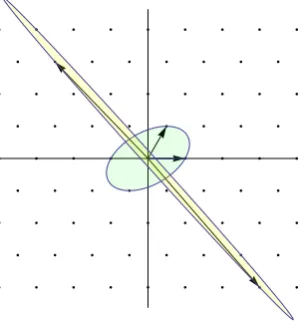
Figure 1: A lattice with two different bases and their fundamental domains, with unit balls for the Eu-clidean and supremum norms.
Definition 2.1. Alatticeis a set of all integral linear combi-nations of a given set of linearly independent points inZn. For
a basisB={b1, . . . ,bd}we denote the lattice it generates by
L(B) =
(
d
∑
i=1
xibi|xi∈Z
)
.
Itsrankisd, and the lattice is said to be offull rankifd=
n. We identify the basis {b1, . . . ,bd} with then×d matrix containingb1, . . . ,bd as columns, which enables us to write
the shorterL(B) =
Bx|x∈Zd .
We use both the termslattice pointandlattice vectorfor ele-ments of a lattice.
1). Indeed, L(B) =L(BU)for any d×d integral matrixU
with det(U) =±1, and any basis ofL(B)is of this formBU. See Figure 1 for a lattice with two different bases.
Associated to a basis Bis itsfundamental domaininRn, given as
Bx|x∈[0,1)d . Any point in the
real span ofBcan be decomposed uniquely into the sum of a lattice point and a point in the fundamental domain. The volumeof a lattice of rankd is thed-dimensional volume of the fundamental domain of a basis. Figure 1 shows in orange shading the fundamental domains for the two bases. It follows that vol(L(B)) =pdet(B>B), and in the full rank case vol(L(B)) =|det(B)|. The volume is independent of the choice of basis, since det((BU)>BU) =det(U>B>BU) =det(U>)det(B>B)det(U) =det(B>B)by det(U) =±1, so for any latticeLthe volume vol(L)is well-defined.
2.2
Norms
Many lattice problems are aboutdistances. The distance between two points is defined as thenormof their difference:d(x,y) =kx−yk, where anorm(also calledlength) onRnis a functionk·k:Rn→Rsatisfying
• kxk>0 for allx∈Rn\ {0}, andk0k=0,
• ktxk=|t|kxkfor allx∈Rn,t∈R,
• kx+yk ≤ kxk+kykfor allx,y∈Rn.
The main example is the Euclidean normkxk2=
√
x>x, but many other examples exist, such as the supre-mum normkxk∞=maxi|xi|forx= (x1, . . . ,xn), thep-normkxkp= (∑i|xi|p)
1/pfor anyp
≥1, and norms coming from inner products. Figure 1 shows unit balls for two norms. Note that for any two norms
k · kα,k · kβ there exists an optimal constantNβ,α such thatk · kβ≤Nβ,αk · kα. Unfortunately this constant
in general depends on the dimension, e.g.N2,∞=
√
n, butN∞,2=1. In particular, for any normk · k∗we defineN∗=N∞,∗. For a matrixMwith columnsmiwe define a norm askMk∗=maxikmik∗. It follows thatkMxk∗≤ kMk∗kxk∞≤N∗kMk∗kxk∗.
The theory of lattice problems and lattice algorithms can be set up for general norms. Let us give a naive example, with a naive solution, just to see what sort of problems will come up. For a given normk · k∗ (that is supposed to be defined on bothRdandRn) and any latticeL, one problem that can be studied is to
determine all lattice points inside a given ball centered around the origin, i.e. to find ally∈Lwithkyk∗≤r, for some radiusr>0. The so-calledGaussian Heuristic[N, Definition 8] says that the number of such points is approximatelyvd∗rd/vol(L), wherevd∗is the volume of thed-dimensional unit ball for the norm
k · k∗. It follows that in order to have any chance of finding a nonzero solution,rmust be at least of the size of vol(L)1/d. For the Euclidean norm it holds [N, Corollary 3] that there is a nonzero solution when
r≥√d·vol(L)1/d. But it may be hard to find it in practice.
When a basisBof the lattice is given, this problem becomes finding allx∈Zdsuch thatkBxk∗≤r. Now note that by definitionB>B is invertible. So fromy=Bx it follows thatx= B>B−1B>y, and thus fromkyk∗≤rit follows that, withF∗(B) =N∗k B>B−1B>k∗, it suffices to search for allx∈Zd with
kxk∗≤F∗(B)r. Brute force techniques then can be invoked to compile a list of all thesex, and each of them can then be further tested forkBxk∗≤r. Note that for full rank lattices,Bitself is invertible, so then
B>B−1B>=B−1, andF
∗(B) =N∗kB−1k∗.
The complexity of this method will be proportional to(F∗(B)r)d. The Gaussian Heuristic says that this is
reasonable when it is approximatelyrd/vol(L)(ignoring minor terms), so that we wantF∗(B)≈vol(L)−1/d.
2.3
Good and bad bases
Assume, for simplicity, that we have a normk · k∗that comes from an inner product, and that we have a basis of full rank (sod=n) that is orthonormal with respect to this norm. Then clearlykB−1k
∗=1, so that
F∗(B) =N∗which is probably not too big, and is anyway independent of the basis. This is a typical example of a ‘good’ basis. A similar argument can be given for ‘orthogonal’ bases, by scaling. Note that for any basis vol(L)≤∏ikbik∗, with equality just for orthogonal bases. In general we can say that a basis is ‘good’ if the number∏ikbik∗/vol(L)is small (i.e. not much larger than 1). On assuming that all basis points have approximately equal norms, this condition becomes even easier, namely thatkBkn
∗/vol(L)is not much bigger than 1. In such a case Cramer’s rule tells us thatkB−1k∗≈ kBkn∗−1/vol(L)≈ kBk−∗1≈vol(L)−1/n, so
that the multiplication factorF∗(B)indeed has the required size vol(L)−1/n, as expected from the Gaussian
Heuristic.
But if we have a basis that is far from orthogonal, in the sense thatkBkn
∗/vol(L)is large, say vol(L)α for someα>0, then the multiplication factorF∗(B)will be of the size of vol(L)α(1−1/n)−1/n, and so with
r≈vol(L)1/nthe complexity of the brute force technique will be vol(L)α(n−1), which is really bad.
As a typical example, look atBε=
p λp qλq+ε
for a very smallε, which has det(Bε) =pε, almost dependent
columns, so is ‘far from good’, andkBεk∗ almost independent ofε, while B−ε1=ε−
1(λq+ε)/p−λ
−q/p 1
,
leading tokB−1
ε k∗growing almost proportional toε−
1.
This simple heuristic argument shows that it will be very useful to have bases as ‘good’ as possible, i.e. as ‘orthogonal’ as possible. But this depends on the norm. We will now show that for every basis a ‘good’ norm can be found easily.
Figure 2: A lattice with unit balls for two differ-ent quadratic form norms.
Indeed, to a (full rank, for convenience) lattice with basisBthe inner product hx,yiB =x>B−1>B−1y can be associated. This inner product defines the associated norm as the square root of a
positive definite quadratic form:kxkB= p
x>B−1>B−1x. This is a very nice norm for this particular basis, because with respect to this inner product the basisBis indeed orthonormal, so the basis is as ‘good’ as possible, as argued above. This shows that for any basis there exist norms for which lattice problems as described above will become relatively easy. See Figure 2 for two different bases with their associated quadratic form norms.
But of course, for all practical purposes, this is not playing fair. In practice one starts with a fixed norm (usually Euclidean), and a lattice is given in terms of a basis that is often quite bad with respect to this given norm. Then, in order to solve lattice prob-lems as described above, one usually needs to first find another basis of the given lattice that is ‘good’ with respect to the given norm. This will lead us to the idea of ‘lattice basis reduction’. Nevertheless it is at least of some historical interest to note that the theory of lattices originated as the theory of positive definite quadratic forms [La], [H].
From now on, for convenience, we will consider only full rank lattices inZd, thus of rankd, with vol(L)
1, and only the Euclidean norm.
In Sections 4 and 5 we will see that there exist algorithms that, on input of any basis of a lattice, however bad, compute a ‘good’ basis B, with a very precise definition of ‘good’. The LLL-algorithm provably reaches (roughly)∏ikbik2/vol(L)≤qd
2
withq=p4
2.4
Gram-Schmidt orthogonalization
As argued above, lattice basis reduction methods try to find good bases from bad ones, and a basis is good when it is as orthogonal as possible. Seeking inspiration from linear algebra then leads one to study the main method for orthogonalization, viz. the well known Gram-Schmidt method. One soon discovers that in the lattice setting it miserably fails, as the process encounters independent points that have perfect orthog-onality properties but with overwhelming probability will lie outside the lattice. Indeed, almost all lattices do not even admit orthogonal bases, so why even bother? Nevertheless, Gram-Schmidt orthogonalization remains a major ingredient of lattice basis reduction methods, so we do briefly describe it here.
LetB={b1, . . . ,bd}be a full rank basis of a latticeLinZd. We recursively define a basisB∗={b∗1, . . . ,b∗d} byb∗1=b1andb∗i =bi−proji(bi)fori≥2, where projiis the orthogonal projection onto the real linear
span ofb1, . . . ,bi−1. Theseb∗i are called theGSO-vectorsof the basisB. Note that the GSO-vectors depend
on the order of the basis vectors, i.e., a different ordering of the basis vectors leads to completely different GSO-vectorsB∗. ClearlyB∗is an orthogonal basis, but with overwhelming probabilityL(B∗)6=L(B), and most likelyL(B∗)is not even inZd. The formula for the projection is proj
i(bi) =∑ij−=11µi,jb∗j, where the
coefficientsµi,jare theGram-Schmidt coefficients, defined byµi,j= (bi·b∗j)/kb∗jk2for 1≤j<i≤d. We
define theGS-transformation matrixas
GB=
1 µ2,1 . . . µd,1 0 1 . .. ...
..
. . .. . .. . .. ... ..
. . .. 1 µd,d−1 0 . . . 0 1
.
Clearly it satisfiesB∗GB=B. As det(GB) =1 andB∗is orthogonal, vol(L) =∏ikb∗ik.
2.5
Minkowski’s successive minima and Hermite’s constants
Any latticeLof rank at least 1 has, by its discreteness property, a nonzero lattice point that is closest to the origin. Its norm is the shortest distance possible between any two lattice points, and is called thefirst successive minimumλ1(L)of the lattice. In other words,λ1(L) =min{kxk |x∈L,x6=0}. Minkowski introduced this concept [Min], and generalized it to other successive minima, as follows.
Definition 2.2. Fori=1, . . . ,dtheith successive minimum of the latticeLof rankdis
λi(L) =min{max{kx1k, . . . ,kxik} |x1, . . . ,xi∈Lare linearly independent}.
Another way to defineλi(L)is as min{r>0|dim span(L∩rU)≥i}, whereU is the unit ball in the Eu-clidean norm.
One might think that any lattice should have a basis of which the norms are precisely the successive minima, but this turns out to be wrong. It may happen that all independent sets of lattice points of which the norms are precisely the successive minima generate proper sublattices [N, pp. 32–33].
Hermite discovered thatλ1(L)can be upper bounded by a constant times vol(L)1/d, where the constant
depends only on the rankd, and not on the latticeL. We do not treat Hermite’s constants in this paper, see Nguyen’s paper [N, pp. 33–35] for a brief account. There is no similar result for higher successive minima on their own, but Hermite’s result can be generalized for products of the firstksuccessive minima:
2.6
Size-reduction
We now turn to an algorithmic viewpoint. The first idea that comes to mind in studying algorithms for lat-tice basis reduction is to get inspiration from the Euclidean Algorithm, since this algorithm is easily adapted to deal with lattice basis reduction in the rank 2 case. It iterates two steps: size-reduction and swapping. Size-reduction of a basis{b1,b2}with, without loss of generality,kb1k ≤ kb2k, means replacingb2 by
b2−λb1, for an optimally chosen integerλ such that the newb2becomes as short as possible. Iteration stops when size-reduction did not yield any improvement anymore, i.e. whenkb1k ≥ kb2khappens. Note that by the integrality ofλ the two bases generate the same lattice at every step in the algorithm. This lat-tice basis reduction algorithm, essentially the Euclidean algorithm but in the case of 2-dimensional bases known as Lagrange’s Algorithm and as Gauss’ Algorithm, is further presented and discussed in Section 4.1 as Algorithm 3.
A generalization to higher dimensions is not immediate, because in both the size-reduction and the swap-ping steps there are many basis vectors to choose from, and one needs a procedure to make this choice. For the size-reduction step this is easy to solve: theµi,jin the GS-transformation matrix are approximately the
properλ’s. But we have to take into account that 1) we need to subtract only integer multiples whereasµi,j
probably are not integral, and 2) whenbichanges, then so will allµi,k. The following algorithm does this
size-reduction in the proper efficient way, treating the columns from left to right, and per column bottom up. In this way the Gram-Schmidt vectorsb∗i do not change at all.
Algorithm 1A size-reduction algorithm
Require: a basis{b1, . . . ,bd}ofL
Ensure: the Gram-Schmidt coefficients of the output basis{b1, . . . ,bd} ofLsatisfy |µi,j| ≤12 for each 1≤j<i≤d
1: fori=2 toddo
2: for j=i−1 down to 1do
3: bi←bi− bµi,jebj
4: fork=1 to jdo
5: µi,k←µi,k− bµi,jeµj,k
6: end for
7: end for
8: end for
An obvious way to generalize the swapping step is to order the basis vectors from shortest to longest . This straightforward generalization of the Euclidean algorithm seems not to be the right one, as it is similar to the greedy lattice basis reduction algorithm of Nguyen and Stehl´e [NS1], which is known to be far from optimal. In Section 4 we will see what better algorithms exist.
2.7
Babai’s algorithms
Finding short nonzero points in a lattice can be done, as discussed above, with a lattice basis reduction algorithm followed by a brute force search. Lattice basis reduction is important here, because as we saw, it greatly improves the efficiency of the search phase. Another natural problem to look at is, given a target vectort∈Rd, find a lattice vector close to it, preferably the closest one. It can be seen as the inhomogeneous
version of the problem of finding short nonzero lattice vectors. For solving this problem it also makes sense to first apply a lattice basis reduction algorithm, in order to get a ‘good’, almost orthogonal basis of the lattice. To find a lattice vector close tot, Babai [B] introduced two methods described below. Once a lattice point close totis found, others (say within a certain ball aroundt, or the closest one) can be found by brute force search techniques as described above.
whenBis the reduced basis of the lattice, computeu=B
B−1t
as a lattice point close tot. Babai proved thatku−tk ≤(1+2d(9/2)d/2)min{kz−tk |z∈L(B)}, wheredis the rank ofL(B).
The second method of Babai is thenearest plane algorithm. If the reduced basis of the lattice is{b1, . . . ,bd}, then first find λd∈Zsuch that the hyperplane λdbd+span(b1, . . . ,bd−1)is closest to t. Then replace
tbyt−λdbd, and recursively apply the same method to the basis {b1, . . . ,bd−1}. The resulting lattice vector is ∑iλibi. This idea is written out in Algorithm 2. Babai showed that this algorithm achieves ku−tk ≤2(p4/3)dmin{kz−tk |z∈L(B)}.
Algorithm 2Babai’s nearest plane algorithm
Require: a reduced basis{b1, . . . ,bd}ofL, and a target vectort∈Rd
Ensure: the ouput lattice vectoru∈Lis ‘close’ tot
1: s←t
2: fori=ddown to 1do
3: s←s−λbi, whereλ=b(s·b∗i)/(b∗i ·b∗i)e
4: end for
5: u←t−s
2.8
The Hermite factor and high dimensions
To measure the quality of a lattice basis reduction algorithm, one could look only at the length of the first reduced basis vector. Of course this makes sense only if one is only interested in finding one short nonzero lattice vector, and if the first basis vector is (probably) the shortest of the output basis vectors. The latter is often the case with the lattice basis reduction algorithms used in practice.
The ideal measure to look at would bekb1k/λ1(L), comparing the length of the first basis vector as a candidate short lattice vector to the actual shortest length of a vector in the lattice. This ratio is called the
approximation factor. However, in practice, given only a (reduced) basis, one does not yet knowλ1(L), and computing it can be a very difficult task, i.e., possibly as hard as actually finding a shortest vector.
Therefore, in practice it is much easier to replaceλ1(L)by vol(L)1/d(wheredis the rank ofL), which is
easy to compute from a basis, as vol(L)simply is its determinant. The resulting ratiokb1k/vol(L)1/d is called theHermite factor.
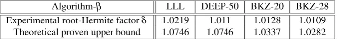
The LLL-algorithm (see Section 4.2) provably reaches a Hermite factor of(p
4/3+ε)(d−1)/2≈1.075d−1 [LLL]. In practical experiments, for high dimensions, it even appears to reach 1.02d−1[GN]. The algorithm BKZ-20 (see Section 4.4) even reaches 1.012(d−1)/2[GN].
At first sight these results seem to be pretty good. For small dimensions this is indeed the case, as the Hermite factors stay close to 1, making the brute force search procedures quite efficient. However, when the dimensiondgrows, the Hermite factor 1.012d−1grows, first almost linearly like 1+0.012d, but when
d grows the exponential behaviour takes over more and more. For d=500 the factor is already larger than 450, which cannot be called close to 1 any more. Moreover, as this factor describes the radius of the ball in which one has to do the search, and brute force search by its very nature is exponential in the radius, it will become clear that even a Hermite factor very close to 1 (like a hypothetical 1.0001) will for high enough dimensions turn out to become a real obstacle, leading to superexponential search complexity. These heuristics should provide the reader with some crude intuition why lattice problems are thought to be hard problems, so that cryptosystems can be based on them. Section 6 elaborates on these issues.
3
Hard Lattice Problems
and cryptanalysis of the cryptosystem. If both the hardness of the lattice problem and the relation to attack methods for the cryptosystem are well enough understood, key size recommendations may be established (or, in the worst case, the cryptosystem may be considered completely broken). The focus in this section is on the hard lattice problems themselves, not on cryptosystems and relations between the two. An overview of hard lattice problems and their interconnections is presented. This section is loosely based on [Pol, Sections 1.4, 1.6, 3.1]
In this section,Lis a full rank lattice inZd.
3.1
Finding short vectors
We recall thefirst successive minimumof the latticeL, which is the length of the shortest nonzero lattice vector (or, stated differently, the minimal distance between two lattice points), i.e.,λ1(L) =min{kxk |x∈
L,x6=0}. The first obvious problem in lattice theory is to find a nonzero lattice vector that reaches this minimum. Note that it is never unique, ask(−x)k=kxkfor all lattice vectorsx∈L(there may be other lattice points with the same norm).
SVP – The Shortest Vector Problem
Given a basis ofL, findy∈Lsuch thatkyk=λ1(L).
Often applications need only sufficiently short lattice points. This gives rise to the following relaxation of SVP.
SVPγ– The Approximate Shortest Vector Problem
Given a basis ofLand an approximation factorγ≥1, findy∈Lsuch that 0<kyk ≤γ λ1(L).
Clearly SVP = SVP1. SVPγis known to be NP-hard forγ=2log
1/2−ε(d)
≈√d[Kh].
Note that in the above problems,λ1(L)is not known in advance. Computing it exactly is the problem SLP = SLP1, described below. But, as remarked in Section 2.8, vol(L)is known, and can be used instead. This gives rise to a ‘Hermite’ variant of (Approximate) SVP.
HSVPγ– The Hermite Shortest Vector Problem
Given a basis ofLand an approximation factorγ>0, findy∈Lsuch that 0<kyk ≤γvol(L)1/d.
As noted in Section 2.8, LLL solves HSVPγ (in polynomial time) for γ = (
p
4/3+ε)(d−1)/2, and in practice it achievesγ=1.02d. With better algorithms evenγ=1.01dis within reach (see Section 4.4). Next we mention a decision variant of SVP.
DSVP – The Decision Shortest Vector Problem
Given a basis ofLand a radiusr>0, decide whether there exists ay∈Lsuch that 0<kyk ≤r. Is it possible to find the first successive minimum without actually finding a shortest nonzero lattice vector? This problem is not necessarily equivalent to SVP, thus we have the following hard problem.
SLPγ– The Approximate Shortest Length Problem
Given a basis ofLand an approximation factorγ>1, find aλ such thatλ1(L)≤λ ≤γ λ1(L).
In cryptographic applications there is interest in lattices with gaps in the sequence of successive minima. This means that there are smaller rank sublattices with smaller volumes than expected from random lattices, sayL0⊂Lwith rankd0<d, such that vol(L0)1/d0is essentially smaller than vol(L)1/d. In other words, there
USVPγ– The Unique Shortest Vector Problem
Given a basis ofLand a gap factorγ≥1, find (if it exists) the unique nonzero y∈Lsuch that any
v∈Lwithkvk ≤γkykis an integral multiple ofy.
And finally, we mention a problem known as GapSVP.
GapSVPγ– The Gap Shortest Vector Problem
Given a basis ofL, a radiusr>0 and an approximation factorγ>1, return YES ifλ1(L)≤r, return NO ifλ1(L)>γr, and return either YES or NO otherwise.
Such a problem is called apromiseproblem. GapSVPγis NP-hard for constantγ [Kh].
3.2
Finding close vectors
As seen in Section 2, the second obvious problem in lattice theory is to find, for a given target pointt∈Rd,
a lattice point that is closest tot. Note that it may not be unique, but in many cases it will. It makes sense to assume thatt6∈L.
Letd(t,L)denote the distance oft∈Rdto the closest lattice point.
CVP – The Closest Vector Problem
Given a basis ofLand a targett∈Rd, findy∈Lsuch thatkt−yk=d(t,L).
As with SVP, it is in practice not always necessary to know the exact solution to a CVP-instance; often an approximation suffices. Therefore we have the following relaxation of CVP.
CVPγ– The Approximate Closest Vector Problem
Given a basis ofL, a targett∈Rdand an approximation factorγ≥1, findy∈Lsuch thatkt−yk ≤
γd(t,L).
CVP = CVP1 is known to be NP-hard [EB]. CVPγ is known to be NP-hard for any constantγ, and is
probably NP-hard forγ=2log1−εd≈d [ABSS]. Babai’s nearest plane algorithm (see Section 2.6) solves CVPγin polynomial time forγ=2(
p 4/3)d.
There are relations between SVP and CVP. Indeed, SVP can be seen as CVP in suitable sublattices [GMSS]. Given a basis{b1, . . . ,bd}, consider the sublattice generated by the basis wherebjis replaced by 2bj. Then
SVP in the original lattice is essentially the CVP-instance for the targetbjin the sublattice, for some j. It
follows that CVPγis at least as hard as SVPγ.
On the other hand, there is an embedding technique [GGH2] that heuristically converts instances of CVP into instances of SVP. The instances are in different lattices with slightly different ranks but identical volumes. The idea is to expand the basis vectors by a 0-coordinate, and the target vector by a 1-coordinate, and then append the target vector to the basis. Heuristically solving SVP in the expanded lattice solves approximately CVP in the original lattice.
As with SVP there are a number of variants of CVP. First we mention the decision variant.
DCVP – The Decision Closest Vector Problem
Given a basis ofL, a target vectort∈Rdand a radiusr>0, decide whether there exists ay∈Lsuch
thatky−tk ≤r.
There exist cryptosystems, that appear to be based on CVP, but where it is known that the distance between the lattice and the target point is bounded. This leads to the following special case of CVP, which is easier.
BDDα– Bounded Distance Decoding
BDDαbecomes harder for increasingα, and it is known to be NP-hard forα>12
√
2 [LLM].
3.3
Finding short sets of vectors
As the first successive minimum has a straightforward generalization into a full sequence of successive minima, the SVP has a straightforward generalization as well. We recall their definition:
λi(L) =min{max{kx1k, . . . ,kxik} |x1, . . . ,xi∈Lare linearly independent}. SMP – The Successive Minima Problem
Given a basis of L, find a linearly independent set{y1, . . . ,yd}inL such thatkyik=λi(L)for i= 1, . . . ,d.
For an approximation factorγ>1 it is clear how SMPγcan be defined.
A different problem is to find a shortest basis.
SBPγ– The Approximate Shortest Basis Problem
Given a basis ofLand an approximation factorγ≥1, find a basis{b1, . . . ,bd}ofLwith maxikbik ≤
γmin{maxikaik | {a1, . . . ,ad}is a basis ofL}. Again we can define SBP = SBP1.
A problem closely related to SBP is the following.
SIVPγ– The Shortest Independent Vector Problem
Given a basis ofLand an approximation factorγ>1, find a linearly independent set{y1, . . . ,yd}such that maxikyik ≤γ λd(L).
SIVPγis NP-hard forγ=d1/log logd[BS].
3.4
Modular lattices
To introduce the final few hard problems some more notation is needed. A latticeL⊂Zmis calledmodular
with modulusq, orq-ary, ifqZm⊂L. Such lattices are only of interest ifqvol(L). Of interest to us are
modular lattices of the formLA,q={x∈Zm|Ax≡0 (modq)}, whereAis ann×mmatrix with integer
coefficients taken moduloq.
The Small Integer Solutions problem comes from Micciancio and Regev [MR1].
SIS – Small Integer Solutions
Given a modulusq, a matrixA(modq) and aν <q, findy∈Zm such that Ay≡0 (modq)and
kyk ≤ν.
Although this is not formulated here as a lattice problem, it is clear that it is a lattice problem in the lattice
LA,q.
Letqbe a modulus. Fors∈Zn
qand a probability distributionχonZq, letAs,χbe the probability
distribu-tion onZn
q×Zqwith sampling as follows: takea∈Zqnuniform, takee∈Zqaccording toχ, then return
(a,ha,si+e) (modq).
The Learning with Errors problem was posed by Regev [R1].
LWE – Learning With Errors
Givenn,q,χand any number of independent samples fromAs,χ, finds.
Forχthe discrete Gaussian distribution is a good choice.
CVPγ HSVPγ √ γn USVPγ [LM] -[LM] | | [LLLS] o
o BDD1/γ
2,[LM]
m m s s SVPγ γ,[Lo]
L L [GMSS] a a GapSVPγ q n
logn,[LM]
;
;
∗,[MR1]
o o SBPγ √
n,[MG]
=
=
√
n/2,[MG]
--SIVP
γ
√
n,[MG]
O
O
√
n/2,[MG]
m
m ∗,[MR1] //
∗,[R1]
5
5
SISn,q,m,ν
b
b
[SSTX]
--LWE n,q,m,α
∗,[MR2]
m
m
K
K
Figure 3: Relations among lattice problems
(modq)for somey}is a lattice in whichA>sis close tob, so this is a CVP-variant, in fact, a BDD-variant.
DLWE – Decision Learning With Errors
Givenn,q,χand any number of independent samples fromAs,χ, return YES if the samples come from
As,χ, and NO if they come from the normal distribution.
3.5
Reductions between hard problems
To end this section, we indicate relations between the main hard lattice problems presented above. The difficulty of hard problems can sometimes be compared byreductionsbetween those problems. We say that Problem A reduces to Problem B if any method that solves all instances of Problem B can be used to solve the instances of Problem A. If this is the case, then Problem B cannot be easier than Problem A. Said differently, Problem B is at least as hard as Problem A.
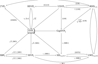
Micciancio and Goldwasser [MG] presented a graphical representation of the relations between the clas-sical Hard Lattice Problems. This inspired us to make a similar picture for what we see as the main Hard Lattice Problems of today, see Figure 3. In this picture, an arrow from Problem A to Problem B means that Problem A can be reduced to Problem B in polynomial time.
A subscriptγ is the approximation factor for SVP, CVP, HSVP, SBP and SIVP, the gap for GapSVP and USVP, and for BDD the subscript 1/γ is the distance bound.
An arrow with a labelα means that the reduction loses a factorα in the subscript. The reductions marked with an asterisk have some more technical conditions attached to them. See Van de Pol’s thesis [Pol, Section 3.1.6] for more details on these reductions, and for references to the relevant literature.
even the reduction of CVPγto SVPγis arguable by the embedding technique. This can be interpreted as
SVPγ being the central hard lattice problem. Therefore in Section 4, algorithms for solving SVPγwill be
the main topic of study.
4
Solving the Approximate Shortest Vector Problem
As we saw in the previous section, the Approximate Shortest Vector Problem is one of the most important hard lattice problems, as many other hard lattice problems can be reduced to this problem. Moreover, as we will see in Section 6, many cryptosystems rely on the hardness of finding (reasonably) short vectors in lattices. Being able to find vectors with sufficiently small approximation factors in these lattices would mean being able to break these cryptosystems. So to estimate the security of these cryptosystems, it is es-sential to understand algorithms for solving approximate SVP, and to be able to quantify their performance for the lattices arising from those cryptosystems.
In this section we will look at several algorithms for solving approximate SVP. The algorithms described in this section are alllattice basis reduction algorithms; instead of outputting a single short vector, these algorithms produce an entire basis of reasonably short vectors. However, to evaluate the quality of the algorithms, we will focus on the length of the shortest vector of the output basis (typicallyb1), and the associated approximation factorkb1k/λ1(L)and Hermite factorkb1k/vol(L)1/d.
In Section 4.1, we first look at Gauss’ algorithm for finding an optimal basis in 2 dimensions. By consid-ering a relaxation and blockwise application of this algorithm, in Section 4.2 we naturally end up with the celebrated LLL algorithm for finding reasonably short vectors in higher dimensions in polynomial time. In Section 4.3, we will then look at KZ-reduction and an algorithm to find KZ-reduced bases inkdimensions, and consider a similar relaxation and blockwise application in Section 4.4, to end up with Schnorr’s hier-archy of basis reduction algorithms, and Schnorr and Euchner’s famous BKZ algorithm. From the BKZ algorithm, it will also become clear why it is important to analyze algorithms for solving the exact shortest vector problem, which is done in the next section. Finally, in Section 4.5 we give a brief overview of the algorithms discussed in this section, and how they relate to each other.
4.1
Gauss’ algorithm
We will start with an easy problem: Finding a basis{b1,b2}for a 2-dimensional latticeLsuch thatkb1k= λ1(L)andkb2k=λ2(L). We can solve this problem withGauss’ algorithm[Ga], given in Algorithm 3, which is sometimes also attributed to Lagrange [La]. In this algorithm we assume that at any point, the Gram-Schmidt coefficientµ2,1= (b2·b1)/kb1k2is known and up to date with respect to the current vectors
b1andb2. For simplicity, and to focus on the high-level description rather than the low-level details, in the algorithms discussed in this section we will omit details on updating the GSO-vectors b∗i and the coefficientsµi,j.
Algorithm 3Gauss’ basis reduction algorithm
Require: a basis{b1,b2}ofL
Ensure: the output basis{b1,b2}ofLsatisfies|µ2,1| ≤ 12andkb1k ≤ kb2k 1: b2←b2− bµ2,1eb1
2: whilekb1k ≥ kb2kdo 3: swap(b1,b2) 4: b2←b2− bµ2,1eb1 5: end while
This algorithm is closely related to Euclid’s greatest common divisor algorithm [E], as was already men-tioned in Section 2.6. At each iteration, we subtract the shortest of the two vectors (b1) an integal number of times (bµ2,1e=b(bk1b·b2)
and we swapb1andb2. In Euclid’s greatest common divisor algorithm, for inputsaandbwitha<b, we also subtract the smallest of the two numbers (a) an integral number of times (bµc=baa·2bc) from the largest
of the two (b) to obtain a smaller numberb←b− bµca. But while in Euclid’s algorithm we usually con-tinue untilb=0, Gauss’ algorithm stops ‘halfway’, as soon askb1k ≥ kb2k. This variant of the Euclidean algorithm is also known in the literature as the half-GCD algorithm.
When Gauss’ algorithm terminates, we know that|µ2,1| ≤12, and the resulting basis{b1,b2}then satisfies the properties described below.
Theorem 4.1. Given a basis{b1,b2}of a lattice L as input, Gauss’ algorithm terminates inpoly(logkBk)
time (i.e., in time polynomial in the size of the input basisB) and outputs a basis{b1,b2}of L satisfying:
kb1k λ1(L)
=1, kb1k
vol(L)1/2 ≤
√
γ2=
4
r 4
3≈1.0746,
kb∗1k kb∗2k≤
r 4
3. (4.1)
Let us briefly explain where the Hermite factorγ2= p
4/3 comes from. We know that for the Gram-Schmidt orthogonalization of the output basis{b1,b2}, we haveb∗1=b1and|µ2,1| ≤12, and we know that the output basis satisfieskb2k ≥ kb1k. So we get a lower bound on the ratio between the norms ofb∗2and
b∗1as
kb∗2k2
kb∗1k2=
kb2−µ2,1b1k2
kb1k2 ≥
kb2k2−µ22,1kb1k2
kb1k2 ≥
1−µ22,1≥3 4. The result then follows from the fact that vol(L) =kb∗1k · kb∗2k.
Note that the upper bounds in (4.1) are sharp for lattices of rank 2 in general, since thehexagonal lattice, spanned by the vectorsb1= (1,0)andb2= (12,12
√
3), attains these bound. This lattice is shown in Figures 1 and 2.
4.2
The LLL algorithm
By applying Gauss’ algorithm to a basis{b1,b2}, we are basically ensuring that the ratio between the two GSO-vectors,kb∗2k2/kb∗
1k2≥1−µ22,1≥ 3
4, cannot be too small. Since the volume of the lattice is the product of the norms of the GSO-vectors, the volume is then bounded from below by a constant times
kb∗1kd. This is also the main idea behind (the proof of) theLenstra-Lenstra-Lov´asz (LLL) algorithm[LLL],
which is essentially a blockwise, relaxed application of Gauss’ algorithm to higher-dimensional lattices. Given a basis{b1, . . . ,bd}of ad-dimensional latticeL, we want to make sure that for eachifrom 2 tod, the ratio between the lengths of the consecutive Gram-Schmidt vectorsb∗i andb∗i−1is sufficiently large. The most natural choice for a lower bound on these values would be 1−µi2,i−1≥34, but with this choice, no one has been able to find an algorithm with a provable polynomial runtime. To ensure a polynomial time complexity, Lov´asz therefore introduced a slight relaxation of this condition. Forδ∈(14,1), and for eachi between 2 andd,Lov´asz’ conditionis defined as
kb∗ik2
kb∗i−1k2 ≥δ−µ 2
i,i−1. (4.2)
The LLL algorithm can be summarized as applying Gauss’ algorithm iteratively to each pair of vectors
bi,bi−1, forifrom 2 tod, ensuring that each pair of vectorsbi,bi−1satisfies the Lov´asz condition. The algorithm also makes sure that the basis is size-reduced at all times. When we swap two vectorsbi and bi−1, we may ruin the relation betweenb∗i−1andb∗i−2, so each time we swap two vectors, we decreasei by 1 to see if we need to fix anything for previous values ofi. This leads to the LLL algorithm given in Algorithm 4. Note that takingd=2 andδ =1 leads to Gauss’ 2-dimensional reduction algorithm, so the LLL algorithm could be seen as a generalization of Gauss’ algorithm.
Algorithm 4The Lenstra-Lenstra-Lov´asz (LLL) basis reduction algorithm
Require: a basis{b1, . . . ,bd}ofL, and a constantδ ∈(14,1)
Ensure: the output basis{b1, . . . ,bd}ofLsatisfies (4.2) for eachifrom 2 tod
1: i←2
2: whilei≤ddo
3: bi←bi−∑ij−=11bµi,jebj
4: ifkb∗ik2≥(δ−µi2,i−1)kb∗i−1k2then
5: i←i+1 6: else
7: swap(bi,bi−1) 8: i←max{2,i−1}
9: end if
10: end while
respect to the current basis{b1, . . . ,bd}, even though in lines 3 (when a basis vector is changed) and 7 (when two basis vectors are swapped), this Gram-Schmidt orthogonalization is changed. In practice, we have to update the values ofµi,jandb∗i accordingly after each swap and each reduction. Fortunately, these
updates can be done in polynomial time.
One can prove that the LLL algorithm runs in polynomial time, and achieves certain exponential approxi-mation and Hermite factors. Theorem 4.2 formally describes these results.
Theorem 4.2. Given a basis{b1, . . . ,bd}of a lattice L and a constantδ ∈(14,1)as input, the LLL
algo-rithm terminates inpoly(d,(1−δ)−1,logkBk)time and outputs a reduced basis{b1, . . . ,bd}of L
satisfy-ing:
kb1k λ1(L)≤
1
δ−14
!(d−1)/2
, kb1k
vol(L)1/d ≤
1
δ−14
!(d−1)/4
.
In particular, forδ =1−ε≈1for small values ofε, the LLL algorithm terminates inpoly(d,1/ε)time and outputs a basis{b1, . . . ,bd}satisfying:
kb1k λ1(L)≤
4 3+O(ε)
(d−1)/2
≈1.1547d−1, kb1k
vol(L)1/d ≤
4 3+O(ε)
(d−1)/4
≈1.0746d−1.
While it may be clear that the Hermite factor comes from repeatedly applying the Lov´asz condition and using vol(L) =∏di=1kb∗ik, at first sight it is not easy to see why this algorithm runs in polynomial time.
We give a sketch of the proof here. First, let us assume that the basis vectors are all integral, and consider
the quantityN=∏di=1kb∗ik2(d−i+1). SinceN can equivalently be written asN=∏dj=1
∏ij=1kb∗ik2
=
∏dj=1vol({b1, . . . ,bj})2, it follows thatN∈N. Now if we investigate what happens when we swap two
vectorsbiandbi−1in line 7, we notice that this quantityN decreases by a factor of at leastδ. It follows that the number of swaps is at most logarithmic inN. Finally, sinceN≤maxikbik2d=kBk2dis at most
exponential ind, the number of iterations is at most polynomial ind.
4.2.1 Improvements for the LLL algorithm
Since the publication of the LLL algorithm in 1982, many variants have been proposed, which in one way or another improve the performance. One well-known variant of the LLL algorithm is usingdeep insertions, proposed by Schnorr and Euchner in 1994 [SE]. Instead of swapping the two neighboring basis vectorsbiandbi−1, this algorithm insertsbisomewhere in the basis, at some position j<i. This can be
original LLL algorithm. To choose where to insert the vectorbi, we look for the smallest index jsuch that
inserting the vector at that position, we gain a factor of at leastδ, as in the proof of the LLL-algorithm. So we look for the smallest index jsuch that:
δkb∗jk2>kbik2.
When the algorithm terminates, the notion of reduction achieved is slightly stronger than in the original LLL algorithm, namely:
∀j<i≤d: δkb∗jk2≤
b∗i+ i−1
∑
k=j
µi,kb∗k
2
.
In practice, this slight modification leads to shorter vectors but a somewhat longer runtime. In theory, proving a better performance and proving a polynomial runtime (when the gap between jandiis allowed to be arbitrarily large) seems hard.
Besides theoretical improvements of the LLL algorithm, practical aspects of LLL have also been studied. For example, how does floating-point arithmetic influence the behaviour of the LLL algorithm? Working with floating-point arithmetic is much more efficient than working exactly with rationals, so this is very relevant when actually trying to implement the LLL algorithm efficiently, e.g., as is done in the NTL C++ library [Sho]. When working with floating-point numbers, cancellations of large numbers and loss of precision can cause strange and unexpected results, and several people have investigated how to deal with these problems. For further details, see papers by, e.g., Stehl´e [St], Schnorr and Euchner [SE] or Nguyen and Stehl´e [NS2, NS4].
Finally, let us emphasize the fact that LLL is still not very well understood. It seems to work much better in practice than theory suggests, and no one really seems to understand why. Several papers have investigated the practical performance of LLL on ‘random bases’ to find explanations. For instance, Gama and Nguyen [GN] conducted extensive experiments with LLL and LLL with deep insertions (and BKZ, see Section 4.4), and noticed that the Hermite factor converges to approximately 1.02dfor large dimensionsd. Nguyen and Stehl´e [NS3] studied the configuration of local bases{b∗i,µi+1,ib∗i +b∗i+1}output by the LLL algorithm, and obtained interesting but ‘puzzling’ results in, e.g., [NS3, Figure 4]. Vall´ee and Vera [VV] investigated whether the constant 1.02 can be explained by some mathematical formula, but it seems that this problem is still too hard for us to solve. So overall, it is safe to say that several open problems still remain in this area.
4.3
KZ-reduction
In the previous subsections we focused on 2-dimensional reduction: Gauss’ algorithm, for finding optimal 2-dimensional bases, and the blockwise LLL algorithm, for finding bases in high dimensions that are locally almost Gauss-reduced. In the next two subsections we will follow the same path, but for the more general
k-dimensional setting, fork≥2. First we consider what optimal means, and we give an algorithm for finding these optimal bases inkdimensions. Then we show how to use this as a subroutine in a blockwise algorithm, to obtain lattice bases in high dimensions with smaller exponential approximation factors than the LLL algorithm in a reasonable amount of time. This provides us with a hierarchy of lattice basis reduction algorithms, with a clear tradeoff between the time complexity and the quality of the output basis.
we describe a notion of reduction, together with an algorithm for achieving it, that will give us bases with really small approximation and Hermite factors.
First, with access to an SVP oracle, we can easily let the shortest basis vector b1 of the output basis
{b1, . . . ,bk}satisfykb1k=λ1(L), by choosing the first output basis vector as a shortest vector ofL. We then decompose the vectorsv∈Laccording tov=v1+v2, withv2=α1b1a linear combination ofb1, and
v2∈ hb1i⊥orthogonal tob1. The set of these vectorsv2is also denoted byπ2(L), theprojected latticeof
L, projected over the complement of the linear spanhb1i. Vectors inπ2(L)are generally not in the lattice, but we can alwaysliftany vector inπ2(L)to a lattice vector, by adding a suitable amount ofb1to it. As with the size-reduction technique, this suitable amount can always be chosen between−12 and+1
2. Now, a short vector inπ2(L)does not necessarily correspond to a short lattice vector, but we do know that for size-reduced bases, the following inequality holds:
kbik2=
b∗i + i−1
∑
j=1 µi,jb∗j
2
≤ kb∗ik2+ i−1
∑
j=1
|µi,j|2kb∗jk2≤ kb∗ik2+
1 4
i−1
∑
j=1
kb∗jk2. (4.3)
Instead of finding a vector achieving the second successive minimum ofL, let us now use the SVP oracle on the latticeπ2(L)to find a shortest vector in this projected lattice, and let us treat this shortest vector as the projectionb∗2of some lattice vectorb2. Since the lifting makes sure that the basis{b1,b2}is size-reduced andb1=b∗1is a shortest vector ofL, we can use (4.3) to get an upper bound on the length of the lifted vectorb2as follows:
kb2k2≤ kb∗2k2+ 1 4kb
∗
1k2=λ12(π2(L)) + 1 4λ
2 1(L).
Since the shortest vector in the projected latticeλ1(π2(L))is never longer than the vector achieving the second minimum of the latticeλ2(L), we haveλ1(L),λ1(π2(L))≤λ2(L). So dividing both sides byλ22(L) and using these lower bounds onλ2(L), we get:
kb2k2 λ22(L)≤
4 3.
After findingb2withkb2k=λ1(π2(L)), we repeat the above process withπ3(L), consisting of lattice vec-tors projected onhb1,b2i⊥. We first use an SVP oracle to find a vectorb∗3∈π3(L)withkb∗3k=λ1(π3(L)), and we then lift it to a lattice vectorb3∈L. Applying (4.3) andλ1(L),λ1(π2(L)),λ1(π3(L))≤λ3(L)then gives uskb3k2≤64λ32(L). Repeating this procedure forifrom 4 tok, we thus obtain a basis{b1, . . . ,bk} with, for eachi,kb∗ik=λ1(πi(L)), and:
kbik2
λi2(L)≤
i+3
4 . (4.4)
This notion of reduction, where the Gram-Schmidt vectors of a basis{b1, . . . ,bk}satisfykb∗ik=λ1(πi(L)) for each i, is also called Korkine-Zolotarev (KZ) reduction[KZ], or Hermite-Korkine-Zolotarev (HKZ) reduction, and the bases are called KZ-reduced. The procedure described above, to obtain KZ-reduced bases, is summarized in Algorithm 5. Note that while the LLL algorithm was named after the inventors of thealgorithm, here thenotion of reductionis named after Korkine and Zolotarev. Algorithm 5 is just an algorithm to achieve this notion of reduction.
The following theorem summarizes the quality of the first basis vector, and the ratio between the lengths of the first and last Gram-Schmidt vectors of any KZ-reduced basis. This will be useful for Section 4.4.
Theorem 4.3. Given a basis{b1, . . . ,bk}of a lattice L and an SVP oracleO for up to k dimensions, the
Korkine-Zolotarev reduction algorithm terminates after at most k calls to the SVP oracleOand outputs a reduced basis{b1, . . . ,bk}of L satisfying:
kb1k λ1(L)=1,
kb1k vol(L)1/k ≤
√
γk=O( √
k), kb∗1k
kb∗kk≤k
(1+lnk)/2.
Algorithm 5A Korkine-Zolotarev (KZ) basis reduction algorithm
Require: a basis{b1, . . . ,bk}ofL, and an SVP-oracleOfor up tokdimensions
Ensure: the output basis{b1, . . . ,bk}ofLsatisfieskb∗ik=λ1(πi(L))for eachi∈ {1, . . . ,k}
1: fori=1 tokdo
2: call the SVP oracleOto find a vectorb∗i ∈πi(L)of lengthλ1(πi(L)) 3: liftb∗i into a lattice vectorbisuch that{b1, . . . ,bi}is size-reduced
4: replace the basis vectors{bi+1, . . . ,bk}by lattice vectors{bi+1, . . . ,bk}such that{b1, . . . ,bk}is a
basis forL
5: end for
Note that finding KZ-reduced bases is at least as hard as finding a shortest vector inkdimensions, since the shortest basis vector is a shortest vector of the lattice. So in high dimensions this algorithm and this notion of reduction are impractical. This algorithm only terminates in a reasonable amount of time whenk
is sufficiently small. If we want to find nice bases for arbitraryd-dimensional lattices, for highd, we need different methods.
4.4
The BKZ algorithm
As in Section 4.2, it turns out that we can use the KZ-reduction algorithm as a subroutine for finding nice
d-dimensional bases. If we can make sure that every block ofkconsecutive basis vectors is KZ-reduced, then we can prove strong bounds on the length of the first basis vector. More precisely, if for eachi
from 1 tod−k+1, the lattice πi({bi, . . . ,bi+k−1})(spanned by the vectorsbi, . . . ,bi+k−1 projected on
hb1, . . . ,bi−1i⊥) is KZ-reduced, then the first basis vectorb1satisfies: [Sno1, Theorem 2.3]
kb1k λ1(L)≤α
(d−1)/(2k−2)
k . (4.5)
Proving this is done by comparing the lengths of the pairs of vectorsbi(k−1)andb(i+1)(k−1)−1, foriranging from 1 to dk−−11. For each pair, we use the fact that the block containing these two vectors as first and last vectors is KZ-reduced, to show that their ratio is bounded from above byαk. The product of these ratios
then telescopes to the left hand side of (4.5), while the dk−−11factorsαklead to the right hand side of (4.5),
proving the result.
To get an absolute upper bound on the quality of the first basis vector, we also need a bound onαk. Schnorr
provided one in his 1987 paper [Sno1, Corollary 2.5], by showing thatαk≤k1+lnkfor allk≥2. This means
that if we can achieve the notion of reduction where each localk-block is KZ-reduced and the whole basis is LLL-reduced, then the first basis vector will satisfy
kb1k λ1(L)≤
k12+k−ln2k
d−1
.
Sincek12+k−ln2k →0 for largek, one could also say that
kb1k
λ1(L)≤(1+εk)
d−1,
whereεkis a constant that only depends onkand which converges to 0 askincreases. This means that with
this notion of reduction, one can achieve arbitrarily small approximation factors, and even findshortest
vectors for sufficiently largek. Of course, fork=dthis is trivial, as thenkb1k=λ1(L).
Algorithm 6Schnorr and Euchner’s Block Korkine-Zolotarev (BKZ) basis reduction algorithm
Require: a basis{b1, . . . ,bd}ofL, a blocksizek, a constantδ ∈(14,1), and an SVP-oracleOfor up tok dimensions
Ensure: the output basis {b1, . . . ,bd} of L is LLL-reduced with factor δ and satisfies kb∗ik =
λ1(πi(bi, . . . ,bi+k−1))for eachifrom 1 tod−k+1 1: repeat
2: fori=1 tod−k+1do
3: KZ-reduce the basisπi(bi, . . . ,bi+k−1) 4: size-reduce the basis{b1, . . . ,bd}
5: end for
6: untilno changes occur
For LLL, we could prove a polynomial runtime, because we could find an invariantNwhich always de-creased by a factorδ whenever we ‘did’ something. For the BKZ algorithm, we cannot prove a similar upper bound on the time complexity. The algorithm behaves well in practice, but theoretically it is not known whether (for fixedk>2) the algorithm always terminates in polynomial time. But when the algo-rithm terminates, we do know that the first basis vector is short.
Theorem 4.4. Given a basis{b1, . . . ,bd}of a lattice L and an SVP oracleOfor up to k dimensions, the
Block Korkine-Zolotarev reduction algorithm outputs a basis{b1, . . . ,bd}of L satisfying:
kb1k λ1(L)≤
k12+k−ln2k
d−1
, kb1k
vol(L)1/d ≤ √
γk·
k12+k−ln2k
d−1
.
4.4.1 Improvements for the BKZ algorithm
Some improvements were suggested for BKZ over the years, most of which involve improving the SVP subroutine. For instance, so far the best results seem to have been obtained by using what Chen and Nguyen called BKZ 2.0 [CN]. They used improved enumeration techniques to speed up the algorithm, and to be able to run BKZ with higher blocksizes than was deemed possible before. For more details on this, see Sections 5 and 6.5.
One notable other suggested improvement, which does not involve improving the SVP subroutine, is ter-minating BKZ early, before the algorithm says we are done. It seems that in practice, the early stages of the algorithm lead to the biggest improvements in the quality of the output basis, and so terminating the algorithm early usually gives a basis that is close to BKZ-reduced. For details, see, e.g., the paper of Hanrot, Pujol and Stehl´e [HPS2].
4.5
Relations between basis reduction algorithms
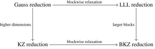
To summarize what we discussed in this section, let us give a basic schematic overview of the different basis reduction algorithms, and their relations. Figure 4 shows the four main algorithms discussed in this section, and how they can be obtained from one another. An arrow from one algorithm to another indicates that the first algorithm is a special case of the second (or, equivalently, the second is a generalization of the first). Choosing the blocksize ask=2 reduces KZ to Gauss and BKZ to LLL, while choosing the dimension asd=kand the “slack” parameter asδ =1 reduces LLL to Gauss, and BKZ to KZ.
5
Solving the Exact Shortest Vector Problem
Gauss reduction
higher dimensions
blockwise relaxation //
LLL reduction
larger blocks
KZ reduction blockwise relaxation //BKZ reduction
Figure 4: A schematic overview of the basis reduction algorithms discussed in this section.
find polynomial time algorithms, but algorithms with a runtime (super)exponential in the dimensiond. But for not too high dimensionsd, computationally this may just be within reach. Besides, we can also use these algorithms in lower dimensions as subroutines for the BKZ algorithm discussed in Section 4.4: with a reasonably fast SVP oracle, we can then use the BKZ algorithm to find short vectors in high dimensional lattices.
For finding a shortest vector in a lattice, several techniques are known. In this section, we will consider the two techniques which currently seem the most promising. In Section 5.1, we look at the most natu-ral approach to this problem, which is enumerating all possible short combinations of basis vectors. By considering all combinations up to a fixed length, the shortest one found is guaranteed to be the shortest vector in the lattice. Even though this technique is superexponential, currently it seems to outperform other techniques.
In Section 5.2, we consider a Monte Carlo-style approach to this problem, which consists of making a huge list of short vectors in the lattice. The lattice vectors in this list cover a large portion of the lattice inside a certain ball. From an old result about sphere packings, it follows that this list cannot grow too large, which ultimately results in a high probability that we will eventually find a shortest vector. This algorithm only has an exponential time complexity, which means that eventually (i.e., for sufficiently high dimensions) it will be faster than enumeration. But due to the large constants, the hidden polynomial factors and the exponential space complexity, and the good performance of heuristic enumeration variants, it still has a way to go to be able to compete with current enumeration techniques.
For more details on algorithms for solving the exact shortest vector problem, including an explanation of a third technique of Micciancio and Voulgaris based on Voronoi cells [MV1], see the excellent survey article of Hanrot, Pujol and Stehl´e [HPS1].
5.1
Enumeration
The idea of enumeration dates back to Pohst [Poh], Kannan [Ka] and Fincke-Pohst [FP]. It consists of trying all possible combinations of the basis vectors and noting which vector is the shortest. Since “all possible combinations” means an infinite number of vectors, we need to bound this quantity somehow. Take a latticeLwith basis{b1, . . . ,bd}. LetR>0 be a bound such thatλ1(L)≤R, e.g. R=kb1k. We would like to be able to enumerate all lattice vectors of norm less thanR. As with basis reduction, this enumeration relies on the Gram-Schmidt orthogonalization of the lattice basis. Let{b∗1, . . . ,b∗d} be the GSO-vectors of our basis. Now letu∈Lbe any vector ofLsuch thatλ1(L)≤ kuk ≤R. Recall that every basis vectorbican be written as a sum of Gram-Schmidt vectors:
bi=b∗i+ i−1
∑
Now, using this and the fact thatuis a lattice vector, it is possible to write
u=
d
∑
i=1
uibi= d
∑
i=1
ui b∗i + i−1
∑
j=1 µi jb∗j
!
= d
∑
j=1
uj+ d
∑
i=j+1
uiµi j
!
b∗j.
Representing the lattice vectoruas a sum of Gram-Schmidt vectors allows for a simple representation of projections ofuas well:
πk(u) =πk d
∑
j=1
uj+ d
∑
i=j+1
uiµi j
!
b∗j
!
= d
∑
j=k
uj+ d
∑
i=j+1
uiµi j
!
b∗j.
Furthermore, since the Gram-Schmidt vectors are by construction orthogonal, the squared norms ofuand its projections are given by
kπk(u)k2=
d
∑
j=k
uj+ d
∑
i=j+1
uiµi j
!
b∗j
2 = d
∑
j=k
uj+ d
∑
i=j+1
uiµi j
!2
kb∗jk2. (5.1)
We will use (5.1) to bound the number of vectors that need to be enumerated until a shortest vector is found. Recall that the boundRwas chosen such thatkuk ≤R. Since the projection of a vector cannot be longer than the vector itself, it follows that
kπd(u)k2≤ kπd−1(u)k2≤. . .≤ kπ1(u)k2=kuk2≤R2. (5.2)
Combining (5.1) and (5.2) givesdinequalities of the form
d
∑
j=k
uj+ d
∑
i=j+1
uiµi j
!2
kb∗jk2≤R2, (5.3)
fork=1, . . . ,d.
The enumeration now works as follows. First, use (5.3) to enumerate all vectorsxinπd(L)of norm at most
R. Then, for each vectorx, enumerate all vectors inπd−1(L)of norm at mostRthat project toxby adding the appropriate multiple ofb∗d−1. Repeat this process to enumerate all vectors inπd−2(L)and continue down the sequence of projected lattices until all vectors inπ1(L) =Lhave been enumerated.
Thinking of this enumeration in terms of inequalities, (5.3) can be used to give bounds for the unknowns
ud, . . . ,u1, in that order. The first inequality is given by
u2dkb∗dk2=kπd(u)k2≤R2.
Thus, it follows that−R/kb∗dk ≤ud≤R/kb∗dk. Now, for any fixedud=u0d in this interval, the next
inequality becomes
(ud−1+u0dµd,d−1)2kb∗d−1k2+u0d2kb∗dk2=kπd−1(u)k2≤R2.
This inequality can be rewritten as
(ud−1+u0dµd,d−1)2≤
R2−u0d2kb∗dk2 kbd−1k2 . Taking the square root on both sides shows thatud−1must lie in the interval
−u0dµd,d−1− q
R2−u02
dkb∗dk2 kbd−1k ≤
ud−1≤ −u0dµd,d−1+ q
R2−u02
dkb∗dk2 kbd−1k
Repeating this process leads to an iterative method to derive the interval ofukonceuk+1, . . . ,udare fixed.
To see this, rewrite (5.3) as
uk+ d
∑
i=k+1
uiµik
!2
≤
R2− ∑dj=k+1
uj+∑di=j+1µi jui
2
kb∗jk2
kb∗kk2 .
Thus, for fixeduk+1=u0k+1, . . . ,ud=u0d,ukmust be in the interval
− d
∑
i=k+1
u0iµik−K≤uk≤ − d
∑
i=k+1
u0iµik+K,
where
K=
r
R2−∑d j=k+1
u0j+∑di=j+1µi ju0i
2
kb∗jk2
kb∗kk .
Note that it is possible that the interval forukis empty (or does not contain integers) for fixedu0k+1, . . . ,u0d.
By trying all possible combinations ofu1, . . . ,udthat satisfy the inequalities from (5.3), we obtain all lattice
vectors∑iuibiof norm smaller thanR. Thus, by keeping track of the shortest vector so far, the result will
be a shortest vector in the lattice.
It is perhaps simpler to view the enumeration vectors as a search through a tree where each node corre-sponds to some vector. Thei’th level of the tree (where the 0th level is the root) consists of all vectors of πd−i+1(L), for 0≤i≤d. Letvbe a node on thei’th level of the tree, i.e.,v∈πd−i+1(L). Then, its children consist of all vectorsu∈πd−i+2(L)that get projected ontovwhen applyingπd−i+1, i.e.,v=πd−i+1(u). Thus, the root of the tree consists ofπd+1(L) ={0}, the zero vector. The first level of the tree consists of all vectors inπd(L) =L(b∗d)of norm at mostR, i.e., all multiples ofb∗dof norm at mostR. The second level of the tree consists of the children of nodes on the first level. This continues until leveld, which contains all vectors ofπ1(L) =Lof norm at mostR.
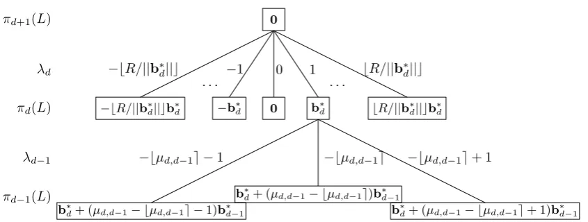
Figure 5 depicts a part of the first two levels of such an enumeration tree. Each block consists of a node containing a vector. The first level contains all integer multiplesλdb∗dsuch that−R/kb∗dk ≤λd≤R/kb∗dk.
On the second level, three children ofb∗dare drawn. These correspond to takingλd=1 in the enumeration
and then takingλd−1in the appropriate interval. If a vectorvis equal tov=λ1b1+. . .+λd−1bd−1+λdbd,
then
πd−1(v) =πd−1(λdbd) +πd−1(λd−1bd−1) =λdb∗d+ (λdµd,d−1−λd−1)b∗d−1.
Note that this is exactly the form of the children of b∗d in the figure. The other children of the node corresponding tob∗dare omitted, as well as the children of the other nodes. Note that the tree is symmetric, as for each vectorvin the tree,−vis in the tree as well. During the enumeration, only one side of the tree needs to be explored.
Such enumeration trees grow quite large. In fact, they become exponentially large, dependent on the pre-cision of the boundR. The lower this bound, the smaller the corresponding enumeration tree. Thus, while such methods give an exact solution to the shortest vector problem, their running time is not polynomially bounded. In order to optimize the running time, lattice basis reduction algorithms are often used before enumerating. This improves the GSO of the basis, reduces the numbersµi jby size-reduction and
addition-ally gives an exponential approximation to the length of a shortest vector (which in turn gives exponential upper bounds for the running time of the enumeration).
Algorithm 7 is a simplified description of the enumeration algorithm. Each node corresponds to a co-efficient vectoru= (u1, . . . ,ud)which corresponds to a lattice vector∑iuibi. The algorithm starts at the