Bootstrapping for HElib

(1)

Bootstrapping for

HElib

∗

Shai Halevi Algorand Foundation

Victor Shoup NYU April 20, 2020

Abstract

Gentry’s bootstrapping technique is still the only known method of obtaining fully homomor-phic encryption where the system’s parameters do not depend on the complexity of the evaluated functions. Bootstrapping involves a recryption procedure where the scheme’s decryption algo-rithm is evaluated homomorphically. Prior to this work there were very few implementations of recryption, and fewer still that can handle “packed ciphertexts” that encrypt vectors of elements. In the current work, we report on an implementation of recryption of fully-packed ciphertexts using the HElib library for somewhat-homomorphic encryption. This implementation required extending previous recryption algorithms from the literature, as well as many aspects of the HElib library. Our implementation supports bootstrapping of packed ciphertexts over many extension fields/rings. One example that we tested involves ciphertexts that encrypt vectors of 1024 elements from GF(216_{). In that setting, the recryption procedure takes under 3 minutes (at}

security-level≈80) on a single core, and allows a multiplicative depth-11 computation before the next recryption is needed.

This report updates the results that we reported in Eurocrypt 2015 in several ways. Most importantly, it includes a much more robust method for deriving the parameters, ensuring that recryption errors only occur with negligible probability. Many aspects of this analysis are proven, and for the few well-specified heuristics that we made, we report on thorough experimentation to validate them. The procedure that we describe here is also significantly more efficient than in the previous version, incorporating many optimizations that were reported elsewhere (such as more efficient linear transformations) and adding a few new ones. Finally, our implementation now also incorporates Chen and Han’s techniques from Eurocrypt 2018 for more efficient digit extraction (for some parameters), as well as for “thin bootstrapping” when the ciphertext is only sparsely packed.

Keywords: Bootstrapping, Homomorphic Encryption, Implementation

∗

(2)

1 Introduction

Homomorphic Encryption (HE) [35, 16] enables computation of arbitrary functions on encrypted data without knowing the secret key. All current HE schemes follow Gentry’s outline from [16], where fresh ciphertexts are “noisy” to ensure security and this noise grows with every operation until it overwhelms the signal and causes decryption errors. This yields a “somewhat homomorphic” scheme (SWHE) that can only evaluate low-depth circuits, which can then be converted to a “fully homomorphic” scheme (FHE) using bootstrapping. Gentry described arecryption operation, where the decryption procedure of the scheme is run homomorphically, using an encryption of the secret key that can be found in the public key, resulting in a new ciphertext that encrypts the same plaintext but has smaller noise.

The last decade saw a large body of work improving many aspects of homomorphic encryption in general and recryption in particular, as well as a multitude of implementations of practically usable homomorphic encryption. Some of those implementations even support bootstrapping, most of which were subsequent to the initial report of this work. Early implementations of recryption prior to our work include the Gentry-Halevi implementation of Gentry’s cryptosystem [17, 16], the implementation of Coron et al. of the DGHV scheme over the integers [11, 6, 12, 14], and the Rohloff-Cousins implementation of the NTRU-based cryptosystem [36, 29, 31].

Here we report on our implementation of recryption for the cryptosystem of Brakerski, Gentry and Vaikuntanathan (BGV) [4]. We implemented recryption on top of the open-source libraryHElib [26, 23], which implements the ring-LWE variant of BGV. Our implementation includes both new algorithmic designs as well as re-engineering of some aspects ofHElib. As noted in [23], the choice of homomorphic primitives inHElib was guided to a large extent by the desire to support recryption, but nonetheless in the course of our implementation we had to extend the implementation of some of these primitives (e.g., matrix-vector multiplication), and also implement a few new ones (e.g., polynomial evaluation).

TheHEliblibrary is “focused on effective use of the Smart-Vercauteren ciphertext packing tech-niques [38] and the Gentry-Halevi-Smart optimizations [19],” so in particular we implemented recryp-tion for “fully-packed” ciphertexts. Specifically, our implementarecryp-tion supports recryprecryp-tion of cipher-texts that encrypt vectors of elements from extension fields (or rings). Importantly, our recryption procedure itself has sufficiently low depth so as to allow significant processing between recryptions while keeping the lattice dimension reasonable to maintain efficiency.

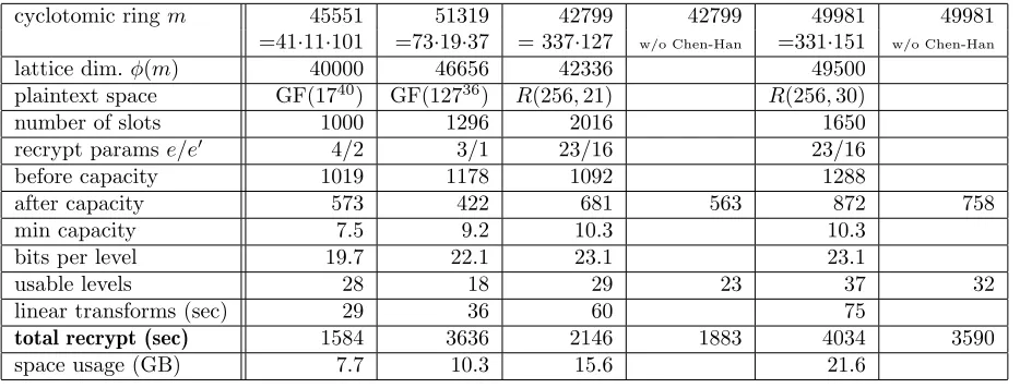
Our experimental results are described in Section 7. Some example settings include: encrypting vectors of 1024 elements from GF(216_{) with a security level of 80 bits, where recryption takes under 3} minutes and allows additional computations of multiplicative depth 11 between recryptions; and en-crypting vectors of 960 elements from GF(224_{) with a security level of 80 bits, where recryption takes} under 5 minutes and allows additional computations of multiplicative depth 15 between recryptions.1 Compared to the previous recrypt implementations, ours offers several advantages in both flex-ibility and speed. Our implementation supports packed ciphertexts that encrypt vectors from the more general extension fields (and rings) already supported byHElib. Some examples that we tested include vectors over the fields GF(216_{), GF(2}25_{), GF(2}24_{), GF(2}36_{), GF(17}40_{), and GF(127}36_{), as} well as degree-21 and degree-30 extensions of the ringZ256.

1.1 Concurrent and subsequent work

Concurrently with our work, Ducas and Micciancio described a new bootstrapping procedure [15]. This procedure is applied to Regev-like ciphertexts [34] that encrypt a single bit, using a secret key

1

(4)

encrypted similarly to the new cryptosystem of Gentry at al. [22]. They reported on an implemen-tation of their scheme, where they can perform a NAND operation followed by recryption in less than a second. This was later improved and extended by Chillotti et al. [9, 10] that implemented bootstrapping in the TFHE library achieving a single-bit recryption speed of 13 milliseconds. While this wall-clock time is much faster than our work, our implementation is about ten times faster in terms of amortized per-bit running time (see below). It remains a very interesting open problem to combine those techniques with ours, achieving a “best of both worlds” implementation.

Another notable subsequent line of work is bootstrapping for the CKKS approximate-number scheme [8, 7, 28, 27], some of which use optimizations that were introduced in the initial version of the current work.

1.1.1 Improvements subsequent to the Eurocrypt 2015 paper

Since the original publication of our bootstrapping techniques in Eurocrypt 2015 [24], we have made a number of improvements, incorporating many optimizations that were reported elsewhere and adding a few new ones. For example, we have improved our matrix multiplication algorithms significantly, as reported in [25]. We have also significantly improved the overall robustness and efficiency of the noise management inHElib. Some of these techniques are specific to bootstrapping, and we report those here (see Section 6).

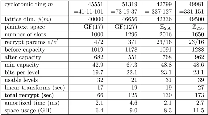
We have also adapted techniques of Chen and Han [5]. In particular, we adapted their techniques for “digit extraction”, which can allow for more noise-efficient bootstrapping (for some parameters). In addition, we adapted their techniques for “thin bootstrapping”, where each slot contains an element of the base field (or ring), rather than an extension field (or ring). This can be advantageous in applications where there is no natural way to exploit the extension field (or ring) structure of the slots. We implemented a variant of their technique, details of which may be found in [25]. We ran various experiments with this “thin bootstrapping” algorithm. For the examples above with plaintext space GF(216_{) and GF(2}24_{) examples mentioned above, if we restrict the plaintext space} to GF(2), the running times drop to 15 and 19 seconds, respectively. In addition, we calculated the “amortized time” for thin bootstrapping, in which we took the total bootstrapping time, divided that by the number of slots, and divided that by the number of usable multiplicative levels between recryptions. In the two examples mentioned above, the “amortized time” of bootstrapping associated with one multiplication GF(2) is about 1.1 milliseconds. If we add to this the amortized time of the multiplication itself (i.e., the multiplication time divded by the number of slots), the total amortized running time per multiplication in GF(2) is about 1.3 milliseconds. In another example, for the plaintext space Z28, we can achieve an amortized time for bootstrapping of 2.1 milliseconds. If we add to this the amortized time of the multiplication itself, the total amortized running time per multiplication inZ28 is about 2.4 milliseconds.

We have also added support for multi-threading toHElib, and have implemented our bootstrap-ping routine to exploit multiple cores when available. In our experiments, with up to 8 cores, we get nearly linear speedup for our bootstrapping routine. For thin bootstrapping, we get somewhat less speedup (see more details in Section 7.2).

1.2 Algorithmic Aspects

Our recryption procedure follows the high-level structure introduced by Gentry et al. [21], and uses the tensor decomposition of Alperin-Sheriff and Peikert [1] for the linear transformations. However, those two works only dealt with characteristic-2 plaintext spaces so we had to extend some of their algorithmic components to deal with characteristicsp >2, see Section 5.

(5)

specialize it to cases that support very-small-depth circuits, and align the different representations to reduce the required data-movement and multiplication-by-constant operations. These aspects are described in Section 4. One significant difference between our implementation and the procedure of Alperin-Sheriff and Peikert [1] is that we do not use the ring-switching techniques of Gentry et al. [18] (see discussion in Appendix 8).

1.3 Organization

We describe our notations and give some background information on the BGV cryptosystem and the HElib library in Section 2. In Section 3 we provide an overview of the high-level recryption procedure from [21] and our variant of it. We then describe in detail our implementation of the linear transformations in Section 4 and the non-linear parts in Section 5. In Section 5.4 we explain how all these parts are put together in our implementation. In Section 6 we describe how various parameters are chosen to ensure a low probability of error. In Section 7 we discuss our performance results. We conclude with directions for future work in Section 9.

2 Notations and Background

For integerz, we denote by [z]q the reduction ofzmoduloqinto the interval [−q/2, q/2), except that forq = 2 we reduce to (−1,1]. This notation extends to vectors and matrices coordinate-wise, and to elements of other algebraic groups/rings/fields by reducing their coefficients in some convenient basis.

For an integer z (positive or negative) we consider the base-prepresentation of z and denote its digits by zh0ip, zh1ip,· · ·. When p is clear from the context we omit the subscript and just write

zh0i, zh1i,· · ·. When p= 2 we consider a 2’s-complement representation of signed integers (i.e., the top bit represents a large negative number). For an oddpwe consider balanced mod-prepresentation where all the digits are in [−p−1₂ ,p−1₂ ].

For indexes 0 ≤ i ≤ j we also denote by zhj, . . . , ii_p the integer whose base-p expansion is zhji · · ·zhii (with zhii the least significant digit). Namely, for odd p we have zhj, . . . , iip =

Pj

k=izhkipk

−i_{, and for} _p _{= 2 we have} _z_h_{j, . . . , i}_i

2 = (Pj_k−1₌_izhki2k−i)−zhji2j−i. The properties of these representations that we use in our procedures are the following:

• For anyr≥1 and any integer z we have z=zhr−1, . . . ,0i (modpr_).

• If the representation ofzisdr−1, . . . , d0then the representation ofz·prisdr−1, . . . , d0, rzeros

z }| {

0,· · ·,0.

• Ifp is odd and |z|< pe_/_{2 then the digits in positions} _e_{and up in the representation of} _z _are all zero.

• Ifp= 2 and |z|<2e−1_{, then the bits in positions} _e₋_{1 and up in the representation of}_z_{, are} either all zero ifz≥0 or all one if z <0.

2.1 The BGV Cryptosystem

The BGV ring-LWE-based somewhat-homomorphic scheme [4] is defined over a ring R def= Z[X]/(Φm(X)), where Φm(X) is the mth cyclotomic polynomial. For an arbitrary integer mod-ulus N (not necessarily prime) we denote the ring RN

def

= R/N R. We often identify elements in R

(6)

As implemented in HElib, the native plaintext space of the BGV cryptosystem is Rpr for a

prime powerpr_{. The scheme uses a large number of different moduli, and a ciphertext relative to} one of these moduli q is a vector ct ∈ (Rq)2. At any point, a ciphertext is defined relative to one modulus, but that modulus keeps changing throughout the computation via mod-up and mod-down operations.

The secret keys are elements s ∈R with “small” coefficients (chosen in {0,±1} in HElib), and we views as the second element of the 2-vector sk= (1,s)∈R2_{. A ciphertext}_ct_{= (}_c

0,c1) encrypts a plaintext element m ∈ Rpr with respect to sk = (1,s) and modulus q if we have [hsk,cti]_q =

[c0+s·c1]q=m+pr·e(inR) for a small noise termpr·e(with norm q).

The noise term grows with homomorphic operations of the cryptosystem, and switching from q

toq0< q is used to decrease the noise term roughly by the ratio q0/q. Once we have a ciphertextct

relative to the smallest modulus, we can no longer use that technique to reduce the noise. To enable further computation, we need to use Gentry’s bootstrapping technique [16], whereby we “recrypt” the ciphertextct, to obtain a new ciphertextct∗ that encrypts the same element ofRpr with respect

to a larger modulus.

In HElib, each modulus q is a product of a number of machine-word sized primes. Elements of the ringRq are typically represented in DoubleCRT format: as a vector of polynomials modulo each small primet, where each of these polynomials is represented by its evaluation at the primitive mth roots of unity inZt. In DoubleCRT format, elements of Rq may be added and multiplied in linear time. Conversion between DoubleCRT representation and the more natural coefficient representation may be effected in quasi-linear time using the FFT.

2.2 Encoding Vectors in Plaintext Slots

As observed by Smart and Vercauteren [38], an element of the native plaintext spaceα∈Rpr can be

viewed as encoding a vector of “plaintext slots” containing elements from some smaller ring extension ofZpr via Chinese remaindering. In this way, a single arithmetic operation onα corresponds to the

same operation applied component-wise to all the slots.

Specifically, suppose the factorization of Φm(X) modulo pr is Φm(X) ≡ F1(X)· · ·Fk(X) (modpr_{), where each} _F

i has the same degreed, which is equal to the order of p modulo m. (This factorization can be obtained by factoring Φm(X) modulopand then Hensel lifting.) From the CRT for polynomials, we have the isomorphism

Rpr ∼=

k

M

i=1

(Z[X]/(pr, Fi(X)).

Let us now define E def= Z[X]/(pr, F1(X)), and let ζ be the residue class of X in E, which is a principal mth root of unity, so that E = Z/(pr)[ζ]. The rings Z[X]/(pr, Fi(X)) for i = 1, . . . , k are all isomorphic to E, and their direct product is isomorphic to Rpr, so we get an isomorphism

between Rpr and Ek. HElib makes extensive use of this isomorphism, representing it explicitly as

follows. It maintains a set S ⊂_Z that forms a complete system of representatives for the quotient group Z∗m/hpi, i.e., it contains exactly one element from every residue class. Then we use a ring isomorphism

Rpr →

M

h∈S

E

α7→ {α(ζh_)} h∈S.

(1)

Here, if α is the residue class a(X) + (pr_,_Φ

(7)

This representation allows HElib to effectively pack k def= |S| = |_Z∗

m/hpi| elements of E into different “slots” of a single plaintext. Addition and multiplication of ciphertexts act on the slots of the corresponding plaintext in parallel.

2.3 Hypercube structure and one-dimensional rotations

Beyond addition and multiplications, we can also manipulate elements in Rpr using a set of

auto-morphisms onRpr of the forma(X)7→a(Xj), or in more detail

τj :Rpr →R_pr

a(X) + (pr,Φm(X))7→a(Xj) + (pr,Φm(X)).

(j∈_Z∗_m)

We can homomorphically apply these automorphisms by applying them to the ciphertext elements and then performing “key switching” (see [4, 19]). As discussed in [19], these automorphisms induce a hypercube structure on the plaintext slots, where the hypercube structure depends on the structure of the group Z∗m/hpi. Specifically, HElib keeps a hypercube basis g1, . . . , gn ∈ Z∗m, together with orders`1, . . . , `n ∈Z>0, and then defines the set S of representatives for Z∗m/hpi (which is used for slot mapping Eqn. (1)) as

S def= {ge1₁ · · ·gen

n : 0≤ei< `i, i= 1, . . . , n}. (2)

Note that ì need not be the order of gi in Z∗m. This basis defines an n-dimensional hypercube structure on the plaintext slots, where slots are indexed by tuples (e1, . . . , en) with 0 ≤ ei < ì. If we fix e1, . . . , ei−1, ei+1, . . . , en, and let ei range over 0, . . . , ì −1, we get a set of ì slots, in-dexed by (e1, . . . , ei, . . . en), which we refer to as ahypercolumn in dimension i(and there are k/ì such hypercolumns). Using automorphisms, we can efficiently perform rotations in any dimension; a rotation by v in dimension i maps a slot indexed by (e1, . . . , ei, . . . , en) to the slot indexed by (e1, . . . , ei+vmodì, . . . , en). Below we denote this operation byρv_i.

We can implementρv

i by applying either one automorphism or two: if the order ofgi inZ∗m is`i, then we get by with just a single automorphism,ρv

i(α) =τgv

i(α). If the order ofgi inZ

∗

m is different from`ithen we need to implement this rotation using two shifts: specifically, we use a constant “0-1 mask value”mask that selects some slots and zeros-out the others, and use two automorphisms with exponents e=gv

i modm and e0 =g v−`i

i modm, setting

ρv_i(α) =τe(mask·α) +τe0((1−mask)·α).

In the first case (where one automorphism suffices) we call ia “good dimension”, and otherwise we callia “bad dimension”.

2.4 Frobenius and linearized polynomials

We define σ def= τp, which is the Frobenius map on Rpr. It acts on each slot independently as the

Frobenius map σE on E, which sends ζ to ζp and leaves elements of Zpr fixed. (When r = 1, σ is

the same as the pth power map on E.) For any Zpr-linear transformation on E, denoted M, there

exist unique constantsθ0, . . . , θd−1 ∈E such that M(η) =P_fd−1₌₀θfσEf(η) for allη ∈E. Whenr= 1, this follows from the general theory of linearized polynomials (see, e.g., Theorem 10.4.4 on p. 237 of [37]), and these constants are readily computable by solving a system of equations modp; the case of

r >1 is similar, and can be thought of as Hensel-lifting these mod-p solutions to a solution modpr_.

In the special case where the image ofM is the sub-ringZpr ofE, the constantsθ_f are obtained as

(8)

Using linearized polynomials, we may effectively apply a fixed linear map to each slot of a plaintext elementα∈Rpr (either the same or different maps in each slot) by computingPd−1

f=0κfσf(α), where theκf’s are Rpr-constants obtained by embedding appropriate E-constants in the slots.

3 Overview of the Recryption Procedure

Recall that the recryption procedure is given a BGV ciphertext ct = (c₀,c₁), defined relative to secret-keysk = (1,s), modulus q, and plaintext space pr_{, namely, we have [h}_sk,_ct_i]

q ≡m (modpr) withmbeing the plaintext. Also we have the guarantee that the noise inct is still rather small.

The goal of the recryption procedure is to produce another ciphertextct∗ that encrypts the same plaintext elementmrelative to the same secret key, but relative to a much larger modulusQqand with a much smaller relative noise. Our implementation uses roughly the same high-level structure for the recryption procedure as in [21, 1], below we briefly recall the structure from [21] and then describe our variant of it.

3.1 The GHS Recryption Procedure

The recryption procedure from [21] (for plaintext spacep= 2) begins by using modulus-switching to compute another ciphertext that encrypts the same plaintext asct, but relative to a specially chosen modulus ˜q= 2e_{+ 1 (for some integer}_e_).

Denote the resulting ciphertext byct0, the rest of the recryption procedure consists of homomor-phic implementation of the decryption formulam←[[hsk,ct0i]q˜]2, applied to an encryption ofskthat can be found in the public key. Note that in this formula we knowct0= (c0₀,c0₁) explicitly, and it issk

that we process homomorphically. It was shown in [21] that for the special modulus ˜q, the decryption procedure can be evaluated (roughly) by computingu←[hsk,ct0i]₂e+1 and thenm←uhei ⊕uh0i.2

To enable recryption, the public key is augmented with an encryption of the secret keys, relative to a (much) larger modulusQq˜,and also relative to a larger plaintext space2e+1_{. Namely this is} a ciphertext ˜ctsuch that [hsk,ct˜i]Q=s (mod 2e+1). Recalling that all the coefficients inct0 = (c00,c01) are smaller than ˜q/2 <2e+1_/_{2, we consider} _c0

0,c01 as plaintext elements modulo 2e+1, and compute homomorphically the inner-productu←c0₁·s+c0₀ (mod 2e+1_{) by setting}

˜

ct0 ←c0₁·ct˜ + (c0₀,0).

This means that ˜ct0 encrypts the desiredu, and to complete the recryption procedure we just need to extract and XOR the top and bottom bits from all the coefficients in u, thus getting an encryption of (the coefficients of) the plaintext m. This calculation is the most expensive part of recryption, and it is done in three steps:

Linear transformation. First apply homomorphically a Z2e+1-linear transformation to ˜ct 0

, con-verting it into ciphertexts that have the coefficients ofu in the plaintext slots.

Bit extraction. Next apply a homomorphic (non-linear) bit-extraction procedure, computing two ciphertexts that contain the top and bottom bits (respectively) of the integers stored in the slots. A side-effect of the bit-extraction computation is that the plaintext space is reduced from mod-2e+1 _to mod-2, so adding the two ciphertexts we get a ciphertext whose slots contain the coefficients of m

relative to a mod-2 plaintext space.

2

(9)

Inverse linear transformation. Finally apply homomorphically the inverse linear transformation (this time overZ2), obtaining a ciphertext ct∗ that encrypts the plaintext element m.

An optimization. The deepest part of recryption is bit-extraction, and its complexity — both time and depth — increases with the most-significant extracted bit (i.e., withe). The parameter e

can be made somewhat smaller by choosing a smaller ˜q = 2e_{+ 1, but for various reasons ˜}_q _cannot be too small, so Gentry et al. described in [21] an optimization for reducing the top extracted bit without reducing ˜q.

After modulus-switching to the ciphertext ct, we can add multiples of ˜q to the coefficients of

c0₀,c0₁ to make them divisible by 2e0 _{for some moderate-size}_e0 _{< e}_{. Let}_ct00_{= (}_c00

0,c001) be the resulting ciphertext, clearly [hsk,ct0i]q˜= [hsk,ct00i]q˜ so ct00 still encrypts the same plaintext m. Moreover, as long as the coefficients of ct00 are sufficiently smaller than ˜q2_{, we can still use the same simplified} decryption formulau0←[hsk,ct00i]2e+1 and m←u0hei ⊕u0h0i.

However, sincect00 is divisible by 2e0

then so isu0. For one thing this means thatu0h0i= 0 so the decryption procedure can be simplified tom←u0hei. But more importantly, we can dividect00 by 2e0 and compute insteadu00←[hsk,ct00/2e0_i]

2e−e0+1 and m←u0he−e0i. This means that the encryption ofsin the public key can be done relative to plaintext space 2e−e0 _{and we only need to extract}_e₋_e0 bits rather thane.

3.2 Our Recryption Procedure

We optimize the GHS recryption procedure and extend it to handle plaintext spaces modulo arbitrary prime powers pr _{rather than just} _p _{= 2,} _r _{= 1. The high-level structure of the procedure remains} roughly the same.

To reduce the complexity as much as we can, we use a special recryption key ˜sk= (1,˜s), which is chosen as sparse as possible (subject to security requirements). As we elaborate in Section 6, the number of nonzero coefficients in ˜splays an extremely important role in the complexity of recryption. To enable recryption of mod-pr _{ciphertexts, we include in the public key a ciphertext ˜}_ct _that encrypts the secret key ˜srelative to a large modulusQand plaintext space mod-pe+r _{for some}_{e > r}_. Then given a mod-pr _ciphertext _ct_{to recrypt, we perform the following steps:}

Modulus-switching. Convert ct into another ct0 relative to the special modulus ˜q =pe_{+ 1. We} prove in Lemma 5.1 that for the special modulus ˜q, the decryption procedure can be evaluated by computing u←[hsk,ct0i]_pe+r and thenm←uhr−1, . . . ,0i_p−uhe+r−1, . . . , ei_p (modpr).

Optimization. Add multiples of ˜q to the coefficients ofct0, making them divisible bype0 _{for some}

r≤e0 < ewithout increasing them too much. This is described in Section 5.2. The resulting

cipher-text, which is divisible bype0

, is denotedct00= (c00₀,c00₁). It follows from the same reasoning as above that we can now compute u0 ← [hsk,ct00/pe0_i]

pe−e0+r and then m ← −u0he−e0+r−1, . . . , e−e0ip (modpr_).

Multiply by encrypted key. Evaluate homomorphically the inner product (divided by pe0

),

u0 ←(c0₁·s+c0₀)/pe0

(modpe−e0₊_r

), by setting ˜ct0 ←(c0₁/pe0

)·ct˜ + (c0₀/pe0

,0).The plaintext space of the resulting ˜ct0 is modulope−e0+r_.

(10)

Linear transformation. Apply homomorphically aZ_pe−e0+r-linear transformation to ˜ct

0

, convert-ing it into ciphertexts that have the coefficients ofu0in the plaintext slots. This linear transformation, which is the most intricate part of the implementation, is described in Section 4. It uses a tensor decomposition similar to [1] to reduce complexity, but pays much closer attention to details such as the mult-by-constant depth and data movements.

Digit extraction. Apply a homomorphic (non-linear) digit-extraction procedure, computing r

ciphertexts that contain the digitse−e0₊_r₋_{1 through}_e₋_e0_{of the integers in the slots, respectively,} relative to plaintext space mod-pr_{. This requires that we generalize the bit-extraction procedure from} [21] to a digit-extraction procedure for any prime powerpr _≥_{2, this is done in Section 5.3. Once we} extracted all these digits, we can combine them to get an encryption of the coefficients ofm in the slots relative to plaintext space modulopr_.

Inverse linear transformation. Finally apply homomorphically the inverse linear transforma-tion, this time overZpr, converting the ciphertext into an encryptionct∗ of the plaintext elementm

itself. This too is described in Section 4.

Thin bootstrapping. For “thin bootstrapping”, where each slot contains just an integer, we use the Chen-Han procedure [5], which has a somewhat different structure. See Section 7.1 for a brief description.

4 The Linear Transformations

In this section we describe the linear transformations that we apply during the recryption procedure to map the plaintext coefficients into the slots and back. Central to our implementation is imposing a hypercube structure on the plaintext spaceRpr =_Zpr[X]/(Φ_m(X)) with one dimension per factor

ofm, and implementing the second (inverse) transformation as a sequence of multi-point polynomial-evaluation operations, one for each dimension of the hypercube. We begin with some additional background.

4.1 Algebraic Background

Let m denote the parameter defining the underlying cyclotomic ring in an instance of the BGV cryptosystem with native plaintext space Rpr = _Zpr[X]/(Φ_m(X)). Throughout this section, we

consider a particular factorization m = m1· · ·mt, where the mi’s are pairwise co-prime positive integers. We write CRT(h1, . . . , ht) (withhi ∈ {0, . . . , mi−1}) for the unique elementh∈ {0, . . . , m− 1}satisfying h≡hi (mod mi) (i= 1, . . . , t) for alli= 1, . . . , t.

Lemma 4.1 Letp, mand themi’s be as above, wherep is a prime not dividing any of themi’s. Let

d1 be the order of p modulo m1 and for i= 2, . . . , t let di be the order ofpd1···di−1 modulomi. Then the order ofp modulo m isddef= d1· · ·dt.

Moreover, suppose that S1, . . . , St are sets of integers such that each Si ⊆ {0, . . . , mi−1} forms

a complete system of representatives for Z∗mi/hp

d1···di−1_i_{. Then the set} _S def_{= CRT(}_S

1, . . . , St) forms a complete system of representatives for Z∗m/hpi.

Proof. It suffices to prove the lemma fort= 2. The general case follows by induction on t.

(11)

To this end, let a, b∈S, and assume thatpf_a_≡_b _(mod_m_{) for some nonnegative integer}_f_{. We} want to show thata=b. Now, since the congruencepf_a_≡_b_{holds modulo}_m_{, it holds modulo}_m

1 as well, and by the defining property of S1 and the construction ofS, we must have a≡b (modm1). So we may cancela and b from both sides of the congruence pf_a_≡_b _(mod_m

1), obtaining pf ≡1 (modm1), and from the defining property of d1, we must have d1 |f. Again, since the congruence

pf_a_≡_b _{holds modulo} _m_{, it holds modulo}_m

2 as well, and since d1 |f, by the defining property of

S2 and the construction of S, we must have a≡ b (modm2). It follows that a ≡b (modm), and hencea=b.

The powerful basis. The linear transformations in our recryption procedure make use of the same tensor decomposition that was used by Alperin-Sheriff and Peikert in [1], which in turn relies on the “powerful basis” representation of the plaintext space, due to Lyubashevsky et al. [32, 33]. The “powerful basis” representation is an isomorphism

Rpr =_Z[X]/(pr,Φ_m(X)) ∼= R0_pr

def

= Z[X1, . . . , Xt]/(pr,Φm1(X1), . . . ,Φmt(Xt)),

defined explicitly by the map

PowToPoly:f(X1, . . . , Xt)→f(Xm/m1, . . . , Xm/mt),

namelyPowToPoly :R0_pr →Rpr sends (the residue class of) X_i to (the residue class of) Xm/mi.

Recall that we view an element in the native plaintext spaceRpr as encoding a vector of plaintext

slots from E, where E is an extension ring of Zpr that contains a principal mth root of unity ζ.

Below let us define ζi def

= ζm/mi _for _i _{= 1}_{, . . . , t}_{. It follows from the definitions above that for}

h= CRT(h1, . . . , ht) and α=PowToPoly(α0), we haveα(ζh) =α0(ζ1h1, . . . , ζ ht

t ).

Using Lemma 4.1, we can generalize the above to multi-point evaluation. Let S1, . . . , St and S be sets as defined in the lemma. Then evaluating an element α0 ∈R0_pr at all points (ζ₁h1, . . . , ζ_tht),

where (h1, . . . , ht) ranges overS1× · · · ×St, is equivalent to evaluating the corresponding element in

α∈Rpr at all points ζh, whereh ranges overS.

4.2 The Evaluation Map

With the background above, we can now describe our implementation of the linear transformations. Recall that these transformations are needed to map the coefficients of the plaintext into the slots and back. Importantly, it is the powerful basis coefficients that we put in the slots during the first linear transformation, and take from the slots in the second transformation.

Since the two linear transformations are inverses of each other (except modulo different powers ofp), then once we have an implementation of one we also get an implementation of the other. For didactic reasons we begin by describing in detail the second transformation, and later we explain how to get from it also the implementation of the first transformation.

The second transformation begins with a plaintext element β that contains in its slots the powerful-basis coefficients of some other elementα, and ends with the element α itself. Important to our implementation is the view of this transformation asmulti-point evaluation of a polynomial. Namely, the second transformation begins with an elementβ whose slots contain the coefficients of the powerful basisα0 =PowToPoly(α), and ends with the elementαthat holds in the slots the values

α(ζh_{) =}_α0₍_ζh1 1 , . . . , ζ

ht

t )

(12)

Choosing the representatives. Our first order of business is therefore to match up the sets S

from Eqn. (2) and Lemma 4.1. To facilitate this (and also other aspects of our implementation), we place some constraints on our choice of the parameter m and its factorization.3 _{Recall that we} consider the factorizationm=m1· · ·mt, and denote by di the order ofpd1···di−1 modulomi.

I. In choosingmand themi’s we restrict ourselves to the case where each groupZ∗mi/hp

d1···di−1_i_is cyclic of orderki, and let its generator be denoted by (the residue class of) ˜gi∈ {0, . . . , mi−1}. Then fori= 1, . . . , t, we set Si

def = {˜ge

i modmi: 0≤e < ki}.

We define gi def

= CRT(1, . . . ,1,g˜i,1, . . . ,1) (with ˜gi in the ith position), and use the gi’s as our hypercube basis with the order of gi set to ki. In this setting, the set S from Lemma 4.1 coincides with the set S in Eqn. (2); that is, we have S =Qt

i=1g ei

i modm : 0≤ ei < ki =

CRT(S1, . . . , St).

II. We further restrict ourselves to only use factorizationsm=m1· · ·mtfor which d1 =d. (That is, the order ofpis the same inZ∗m1 as inZm∗ .) With this assumption, we haved2 =· · ·=dt= 1, and moreoverk1 =φ(m1)/dand ki=φ(mi) for i= 2, . . . , t.

Note that with the above assumptions, the first dimension could be either good or bad, but the other dimensions 2, . . . , t are always good. This is because pd1···di−1 _≡ _{1 (mod}_m_{), so also} _pd1···di−1 _≡ ₁ (modmi), and therefore Z∗mi/hp

d1···di−1_i ₌

Z∗mi, which means that the order of gi in Z

∗

m (which is the same as the order of ˜gi inZ∗mi) equalski.

Packing the coefficients. In designing the linear transformation, we have the freedom to choose how we want the coefficients ofα0 to be packed in the slots ofβ. Let us denote these coefficients by

cj1,...,jt where each indexji runs over{0, . . . , φ(mi)−1}, and each cj1,...,jt is inZpr. That is, we have

α0(X1, . . . , Xt) =

X

j1,j2,...,jt

cj1,...,jtX

j1 1 X

j2 2 · · ·X

jt t = X j2,...,jt X j1

cj1,...,jtX

j1 1

X₂j2· · ·Xjt

t.

Recall that we can pack d coefficients into a slot, so for fixed j2, . . . , jt, we can pack the φ(m1) coefficients of the polynomial P

j1cj1,...,jtX

j1

1 into k1 = φ(m1)/d slots. In our implementation we pack these coefficients into the slots indexed by (e1, j2, . . . , jt), for e1 = 0, . . . , k1−1. That is, we pack them into a single hypercolumn in dimension 1.

4.2.1 The Eval Transformation

The second (inverse) linear transformation of the recryption procedure beings with the element β

whose slots pack the coefficients cj1,...,jt as above. The desired output from this transformation is

the element whose slots contain α(ζh_{) for all} _h _∈_S _{(namely the element} _α _{itself). Specifically, we} need each slot ofα with hypercube index (e1, . . . , et) to hold the value

α0 ζg

e₁

1

1 , . . . , ζ g_tet t

= α ζg1e1···g

et t .

Below we denote ζi,ei

def = ζgiei

i . We transform β into α in t stages, each of which can be viewed as multi-point evaluation of polynomials along one dimension of the hypercube.

3

(13)

Stage1. This stage begins with the elementβ, in which each dimension-1 hypercolumn with index (?, j2, . . . , jt) contains the coefficients of the univariate polynomial Pj2,...,jt(X1)

def

= P

j1cj1,...,jtX

j1 1 . We transformβ intoβ1 where that hypercolumn contains the evaluation of the same polynomial in many points. Specifically, the slot ofβ1 indexed by (e1, j2, . . . , jt) contains the valuePj2,...,jt(ζ1,e1).

By definition, this stage consists of parallel application of a particularZpr-linear transformation

M1(namely a multi-point polynomial evaluation map) to each of thek/k1hypercolumns in dimension 1. In other words,M1 maps (k1·d)-dimensional vectors overZpr (each packed into k₁ slots) tok

1-dimensional vectors overE. We elaborate on the efficient implementation of this stage later in this section.

Stages 2, . . . , t. The element β1 from the previous stage holds in its slots the coefficients of the k1 multivariate polynomialsAe1(·) (fore1 = 0, . . . , k1−1),

Ae1(X2, . . . , Xt) def

= α0(ζ1,e1, X2, . . . , Xt) =

X

j2,...,jt

X

j1

cj1,...,jtζ

j1 1,e1

| {z }

slot (e1,j2,...,jt)=Pj₂,...,jt(ζ1,e1) ·X₂j2· · ·Xjt

t.

The goal in the remaining stages is to implement multi-point evaluation of these polynomials at all the points Xi =ζi,ei for 0≤ei < ki. Note that differently from the polynomial α

0 _{that we started} with, the polynomialsAe1 have coefficients fromE (rather than fromZpr), and these coefficients are

encoded one per slot (rather thandper slot). As we explain later, this makes it easier to implement the desired multi-point evaluation. Separating out the second dimension we can write

Ae1(X2, . . . , Xt) =

X

j3,...,jt

X

j2

Pj2,...,jt(ζ1,e1)X

j2 2

X₃j3· · ·Xjt

t .

We note that each dimension-2 hypercolumn in β1 with index (e1, ?, j3, . . . , jt) contains the E -coefficients of the univariate polynomial Qe1,j3,...,jt(X2)

def

= P

j2Pj2,...,jt(ζ1,e1)X

j2

2 . In Stage 2, we transform β1 into β2 where that hypercolumn contains the evaluation of the same polynomial in many points. Specifically, the slot ofβ2 indexed by (e1, e2, j3. . . , jt) contains the value

Qe1,j3,...,jt(ζ2,e2) =

X

j2

Pj2,...,jt(ζ1,e1)·ζ

j2 2,e2 =

X

j1,j2

cj1,...,jtζ

j1 1,e1ζ

j2 2,e2,

and the following stages implement the multi-point evaluation of these polynomials at all the points

Xi =ζi,ei for 0≤ei< ki.

Stages s = 3, . . . , t proceed analogously to Stage 2, each time eliminating a single variable Xs via the parallel application of an E-linear map Ms to each of the k/ks hypercolumns in dimension

s. When all of these stages are completed, we have in every slot with index (e1, . . . , et) the value

α0(ζ1,e1, . . . , ζt,et), as needed.

Implementation and complexity of Eval. The linear transformations Ms for s = 1, . . . , t are implemented using theMatMul1Dand BlockMatMul1Droutines that are implemented inHElib, and which are described in detail in [25].

The linear transformation M1 is implemented using the BlockMatMul1D routine. The running time of this routine depends on a number of factors, but will typically be dominated by the running time of at mostc1

p

(14)

Fors= 2, . . . , t, the linear transformationMsis implemented using theMatMul1Droutine. Again, the running time of this routine depends on a number of factors, but will typically be dominated by the running time of at mostp

φ(ms)+O(1) automorphism operations andφ(ms) constant-ciphertext multiplications. The depth of the computation is one constant-ciphertext multiplication.

The total running time of Evalwill be dominated by the running time of at most

c1

p

φ(m1) +

p

φ(m2) +· · ·+

p

φ(mt) +O(t)

automorphism operations and

c2φ(m1) +φ(m2) +· · ·+φ(mt).

constant-ciphertext multiplications. The depth of theEval computation ist.

4.2.2 The Transformation Eval−1

The first linear transformation in the recryption procedure is the inverse ofEval. This transformation can be implemented by simply running the above stages in reverse order and using the inverse linear mapsM−1

s in place ofMs. The complexity estimates are identical.

4.3 Unpacking and Repacking the Slots

In our recryption procedure we have the non-linear digit extraction routine “sandwiched” between the linear evaluation map and its inverse. However the evaluation map transformations from above maintain fully-packed ciphertexts, where each slot contains an element of the extension ring E (of degree d), while our digit extraction routine needs “sparsely packed” slots containing only integers fromZpr.

Therefore, before we can use the digit extraction procedure we need to “unpack” the slots, so as to get dciphertexts in which each slot contains a single coefficient in the constant term. Similarly, after digit extraction we have to “repack” the slots, before running the second transformation.

Unpacking. Consider the unpacking procedure in terms of the element β ∈ Rpr. Each slot of β

contains an element of E which we write as Pd−1

i=0 aiζi with the ai’s in Zpr. We want to compute

β(0)_{, . . . , β}(d−1)_{, so that the corresponding slot of each} _β(i) _contains _a

i. To obtain β(i), we need to apply to each slot ofβ theZpr-linear mapL_i:E →_Zpr that maps Pd_i₌₀−1a_iζi toa_i.

Using linearized polynomials, as discussed in Section 2.4, we may write β(i) ₌Pd−1

f=0κi,fσf(β), for constants κi,f ∈ Rpr. Given an encryption of β, we can compute encryptions of all of the

σf₍_β_{)’s and then take linear combinations of these to get encryptions of all of the} _β(i)_{’s. This takes} the time of d−1 automorphisms and d2 _{constant-ciphertext multiplications, and a depth of one} constant-ciphertext multiplication.

While the cost in time of constant-ciphertext multiplications is relatively cheap, it cannot be ignored, especially as we have to computed2 _{of them. In our implementation, the cost is dominated} the time it takes to convert an element in Rpr to its corresponding DoubleCRT representation. It

is possible, of course, to precompute and store alld2 _{of these constants in DoubleCRT format, but} the space requirement is significant: for typical parameters, our implementation takes about 4MB to store a single constant in DoubleCRT format, so for example with d= 24, these constants take up almost 2.5GB of space.

This unappealing space/time trade-off can be improved considerably using somewhat more sophis-ticated implementations. Suppose that in the first linear transformation Eval−1, instead of packing the coefficients a0, . . . , ad−1 into a slot as P_iaiζi, we pack them as

P

(15)

normal element. Further, let L0

0 : E → Zpr be the Zpr-linear map that sends η =

P

iaiσiE(θ) to

a0. Then we have L0₀(σ−j₍_η_{)) =} _a

j for j = 0, . . . , d−1. If we realize the map L00 with linearized

polynomials, and if the plaintext γ has the coefficients packed into slots via a normal element as above, then we haveβ(i) ₌Pd−1

f=0κf·σf−i(γ),where theκf’s are constants inRpr. So we have only

dconstants rather thand2_.

To use this strategy, however, we must address the issue of how to modify theEvaltransformation so thatEval−1 will give us the plaintext elementγ that packs coefficients asP

iaiσiE(θ). As it turns out, in our implementation this modification is for free: recall that the unpacking transformation immediately follows the last stage of the inverse evaluation mapEval−1, and that last stage applies Zpr-linear maps to the slots; therefore, we simply fold into these maps the_Zpr-linear map that takes

P

iaiζi toPiaiσEi (θ) in each slot.

It is possible to reduce the number of stored constants even further: since L0₀ is a map from E

to the base ringZpr, then theκ_f’s are related via κ_f =σf(κ₀). Therefore, we can obtain all of the

DoubleCRTs for the κf’s by computing just one for κ0 and then applying the Frobenius automor-phisms directly to the DoubleCRT for κ0. We note, however, that applying these automorphisms directly to DoubleCRTs leads to a slight increase in the noise of the homomorphic computation. We did not use this last optimization in our implementation.

Repacking. Finally, we discuss the reverse transformation, which repacks the slots, taking

β(0)_{, . . . , β}(d−1) _to _β_{. This is quite straightforward: if ¯}_ζ _{is the plaintext element with} _ζ _{in each}

slot, thenβ =Pd−1

i=0 ζ¯iβ(i). This formula can be evaluated homomorphically with a cost in time of

dconstant-ciphertext multiplications, and a cost in depth one constant-ciphertext multiplication.

5 Recryption with Plaintext Space Modulo

p >

2

Below we extend the treatment from [21, 1] to handle plaintext spaces modulop >2. In Sections 5.1 through 5.3 we generalize the various lemmas top >2. In Section 5.4 we explain how these lemmas are put together in the recryption procedure. In Section 6 we discuss the choice of parameters.

5.1 Simpler Decryption Formula

We begin by extending the simplified decryption formula [21, Lemma 1] from plaintext space mod-2 to any prime-power pr_{. Recall that we denote by [}_z_]

q the mod-q reduction into [−q/2, q/2) (except when q = 2 we reduce to (−1,1]). Also zhj, . . . , ii_p denotes the integer whose mod-p expansion consists of digits ithrough j in the mod-p expansion of z (and we omit thep subscript if it is clear from the context).

Lemma 5.1 Let p >1, e > r ≥ 1, and q = pe_{+ 1} _{be integers. Also let} _z _{be an integer such that} bothz/q and[z]q are sufficiently smaller than q in magnitude, specifically |z/q|+|[z]q| ≤(q−1)/2.

• If p is odd then [z]q =zhr−1, . . . ,0i −zhe+r−1, . . . , ei (mod pr).

• If p= 2 then[z]q=zhr−1, . . . ,0i −zhe+r−1, . . . , ei −zhe−1i (mod 2r).

Proof. We begin with the odd-p case. Denote z0 = [z]q, then z = z0 +kq (or in other words

k= (z−z0)/q). Denoting w=z0+k, we therefore have

|w|=|z0(1−1/q) +z/q|<|z0|+|z/q| ≤(q−1)/2 =pe/2. (3)

This means that the mod-prepresentation of whas only 0’s in positions eand up. Writing

(16)

we conclude that the digitse, e+ 1, . . . inz are the same as the digits 0,1, . . . in k (since no carry digits are generated by w). Namely khr−1, . . . ,0i = zhe+r−1, . . . , ei. On the other hand, we havez0 =z−k−pek=z−k (modpr), so it follows that

z0hr−1, . . . ,0i=zhr−1, . . . ,0i −khr−1, . . . ,0i=zhr−1, . . . ,0i −zhe+r−1, . . . , ei (modpr).

The proof for thep= 2 case is similar, but we no longer have the guarantee that the high-order bits of the sumw=z0+kare all zero. From Eqn. (4) we can still deduce thatzhe−1i=whe−1i and

zhe+r−1, . . . , ei=whe+r−1, . . . , ei+khr−1, . . . ,0i (mod 2r).

Since |w|<2e−1_{, then the bits in positions} _e₋_{1 and up in} _w_{are either all zero if} _w_≥_{0, or all} one ifw <0. In particular, this means that

whe+r−1, . . . , ei =

0 ifw≥0 −1 ifw <0

= −whe−1i = −zhe−1i (mod 2r).

Concluding, we therefore have

z0hr−1, . . . ,0i = zhr−1, . . . ,0i −khr−1, . . . ,0i

= zhr−1, . . . ,0i − zhe+r−1, . . . , ei −whe+r−1, . . . , ei

= zhr−1, . . . ,0i −zhe+r−1, . . . , ei −zhe−1i (mod 2r).

Remark. Lemma 5.1 improves upon the corresponding lemma (also Lemma 5.1) in our report from Eurocrypt 2015 [24]. In that lemma, instead of|z/q|+|[z]q| ≤(q−1)/2, we had a pair of inequalities |z/q| ≤q/4−1 and |[z]q| ≤q/4.

5.2 Making an Integer Divisible By pe0

As sketched in Section 3, we use the following lemma to reduce the number of digits that needs to be extracted, hence reducing the time and depth of the digit-extraction step.

Lemma 5.2 Let e0 _≥ ₁ _and _{q > p >} ₁ _{be integers such that} _q _≡ _{1 (mod} _pe0

). Then for every integer z there exist an integerv such that|v| ≤pe0_/₂_{, such that}

z+v·q≡0 (modpe0₎_.

Proof. Letv=−[z]_pe0, so|v| ≤pe

0

/2. Moreover, sinceq ≡1 (modpe0_{), we have}

0≡z+v ≡z+v·q (modpe0).

(17)

Discussion. Recall that in our recryption procedure we have a ciphertext ct that encrypts some

mwith respect to modulus q and plaintext space mod-pr_{, and we use the lemma above to convert it} into another ciphertext ct0 that encrypts the same thing but is divisible bype0_{, and by doing so we} need to extracte0 _{fewer digits in the digit-extraction step.}

Considering the elementsu ← hsk,cti and u0 ← hsk,ct0i (without any modular reduction), since

sk is integral then adding multiples ofq to the coefficients of ct does not change [u]q, and soct and

ct0 still encrypt the same plaintext. However in our recryption procedure we need more: to use our simpler decryption formula from Lemma 5.1, we need to ensure that|u0/q|+|[u0]q| ≤(q−1)/2, where | · |denotes the`∞-norm on the powerful basis.

5.3 Digit-Extraction for Plaintext Space Modulo pr

The bit-extraction procedure that was described by Gentry et al. in [21] and further optimized by Alperin-Sheriff and Peikert in [1] is specific for the case p = 2e_{. Namely, for an input ciphertext} relative to mod-2e _{plaintext space, encrypting some integer} _z _{(in one of the slots), this procedure} computes the ith top bit of z (in the same slot), relative to plaintext space mod-2e−i+1_{. Below we} show how to extend this bit-extraction procedure to a digit-extraction also whenp is an odd prime. The main observation underlying the original bit-extraction procedure, is that squaring an integer keeps the least-significant bit unchanged but inserts zeros in the higher-order bits. Namely, if b is the least significant bit of the integerzand moreoverz=b (mod 2e_),_e_≥_{1, then squaring}_z _{we get}

z2 ₌_b _{(mod 2}e+1_{). Therefore,}_z₋_z2 _{is divisible by 2}e_{, and the LSB of (}_z₋_z2₎_/₂e_{is the}_e_{th bit of}_z_. Unfortunately the same does not hold when using a basep >2. Instead, we show below that for any exponent ethere exists some degree-p polynomial Fe(·) (but not necessarily Fe(X) = Xp) such that whenz=z0 (modpe) thenFe(z) =z0 (mod pe+1). Hencez−Fe(z) is divisible bype, and the least-significant digit of (z−Fe(z))/pe is theeth digit ofz. The existence of such polynomial Fe(X) follows from the simple derivation below.

Lemma 5.3 For every primep and exponent e≥1, and every integer z of the form z=z0+pez1 (with z0, z1 integers, z0∈[p]), it holds that zp=z0 (modp), andzp=z0p (mod pe+1).

Proof. The first equality is obvious, and the proof of the second equality is just by the binomial expansion of (z0+pez1)p.

Corollary 5.4 For every prime p there exist a sequence of integer polynomials f1, f2, . . ., all of degree ≤ p−1, such that for every exponent e ≥ 1 and every integer z = z0+pez1 (with z0, z1 integers,z0 ∈[p]), we have

zp =z0+

e

X

i=1

fi(z0)pi (modpe+1).

Proof. From Lemma 5.3 we know that the mod-pdigits ofzp_modulo-_pe+1_{depend only on}_z

0, so there exist some polynomials in z0 that describe them, fi(z0) = zphiip. Since these fi’s are polynomials fromZp to itself, then they have degree at mostp−1. Moreover, by the 1st equality in Lemma 5.3 we have that the first digit is exactlyz0.

Corollary 5.5 For every prime p and every e≥ 1 there exist a degree-p polynomial Fe, such that for every integers z0, z1 with z0∈[p] and every 1≤e0≤ewe have Fe(z0+pe

0

z1) =z0 (modpe

0₊₁

).

Proof. Denote z = z0+pe

0

z1. Since z = z0 (modpe

0

) then fi(z0) =fi(z) (mod pe

0

). This implies that for alli ≥1 we have fi(z0)pi =fi(z)pi (modpe

0₊₁

(18)

Digit-Extractionp(z, e): // Extracteth digit in base-prepresentation ofz

1.w0,0←z

2. Fork= 0 toe−1 3. y←z

4. Forj= 0 tok

5. wj,k+1←Fe(wj,k) //Fefrom Corollary 5.5, forp= 2,3we haveFe(X) =Xp

6. y←(y−wj,k+1)/p

7. wk+1,k+1←y

8. Returnwe,e

Figure 1: The digit extraction procedure

fi(z)pi = 0 (modpe

0₊₁

). Therefore, settingFe(X) =Xp−Pei=1fi(X)pi we get

Fe(z) =zp− e

X

i=1

fi(z)pi =zp− e0 X

i=1

fi(z0)pi=z0 (modpe

0₊₁

).

We know that forp= 2 we haveFe(X) =X2 for alle. One can verify that also forp= 3 we have

Fe(X) =X3 for all e (when considering the balanced mod-3 representation), but for larger primes

Fe(X)6=Xp.

The digit-extraction procedure. Just like in the base-2 case, in the procedure for extracting the

eth base-pdigit from the integerz=P

izipi proceeds by computing integerswj,k (k≥j) such that the lowest digit inwj,k iszj, and the next k−j digits are zeros. The code in Figure 1 is purposely written to be similar to the code from [1, Appendix B], with the only difference being in Line 5 where we useFe(X) rather than X2.

In our implementation we compute the coefficients of the polynomial Fe once and store them for future use. In the procedure itself, we apply a homomorphic polynomial-evaluation procedure to computeFe(wj,k) in Line 5. We note that just as in [21, 1], the homomorphic division-by-poperation is done by multiplying the ciphertext by the constant p−1 modq, where q is the current modulus. Since the encrypted values are guaranteed to be divisible by p, then this has the desired effect and also it reduces the noise magnitude by a factor of p. Correctness of the procedure from Figure 1 is proved exactly the same way as in [21, 1], the proof is omitted here.

5.3.1 An optimization for p= 2, r ≥2.

As it turns out, for p = 2 we can sometimes extract several consecutive bits a little cheaper than what the procedure above implies. Specifically, it turns out that forp= 2, e≥0 and r ≥2 we can compute the integer zhe+r, . . . , ei by extracting only e+r−1 bits (rather than e+r of them). Specifically, when applying the procedure from Figure 1 (which forp= 2 is identical to the one from [1, Appendix B]), it turns out that we get

zhe+r, . . . , ei= e+r−1

X

j=r

2j−rwj,e+r−1 (mod 2e+r+1).

Note: the above would have been an immediate corollary from the correctness of the bit-extraction procedure if we added the terms 2j−r_w

j,e+r and let the index j go up toe+r, but in this case we can stop one step earlier and the result still holds.

(19)

so as to get more zeros in higher-order bits, without changing the LSB. Recall also that squaring indeed has the desired effect since for anyi≥1 and any bit b and integernwe have (b+ 2i_n₎2 ₌_b (mod 2i+1_{). To prove the optimization, we need two additional observations:}

Observation 1. For any bitb and integer n we have (b+ 2n)4 ₌_b _{(mod 16).}

Note that this isnot a corollary of the squaring property above — that property only givesb (mod 8), but in fact for this particular case we get one extra zero. (This property holds only for that particular step, for later steps we only get one additional zero per squaring.)

Observation 2. After line 7 in Figure 1, we always havez=Pk+1

j=02jwj,k+1.

This can be verified by inspection: we start in line 3 fromy=z, and at every step we subtract one

wj and divide by two, so adding them back with their respective powers of two gives back z.

Correctness now follows: Let us denote wj def

= wj,e+r−1 so we will not have to carry this extra index everywhere. Because of the first observation, thewj’s for j = 0,1, ..., e+r−3 have an extra zero bit, so for these wj’s we have wj = zhji (mod 2e+r−j+1), not just (mod 2e+r−j). Denoting

vj = 2jwj, this means that the only vj’s that potentially have a nonzero bit in position e+r are

ve+r−2 and ve+r−1. Also by correctness, for lower bit positions j < e+r, only vj potentially has nonzero bit in positionj, and all the other vj’s have zero in that position. Namely, we have

bit position: ? e+r e+r−1 e+r−2 e+r−3 . . . 1 0

v0 =w0= ? 0 0 0 0 0 zh0i

v1= 2w1= ? 0 0 0 0 zh1i 0

..

. ...

ve+r−3 = 2e+r−3we+r−3= ? 0 0 0 zhe+r−3i 0 0

ve+r−2 = 2e+r−2we+r−2= ? σ 0 zhe+r−2i 0 0 0

ve+r−1 = 2e+r−1we+r−1= ? τ zhe+r−1i 0 0 0 0

for some two bitsσ, τ (where the ?’s are bits above position e+r, which we do not care about). This means that when addingPe+r−1

j=0 vj, we have no carry bits up to position e+r. But by the second observation the sum of all thesevj’s isz, so the two top bitsσ, τ must satisfyσ⊕τ =zhe+ri. We conclude that when addingPe+r−1

j=e vj, we get all the bitszhe+r, . . . , eiwhich is what we needed to prove.

5.4 Putting Everything Together

Having described all separate parts of our recryption procedure, we now explain how they are com-bined in our implementation.

Initialization and parameters. Given the ring parameterm (that specifies themth cyclotomic ring of integers R = Z[X]/(Φm(X))) and the plaintext space pr, we compute the recryption pa-rameters as explained in Section 6. That is, we set the exponents e, e0 _{from Lemmas 5.1. We} also precompute some key-independent tables for use in the linear transformations, with the first transformation using plaintext spacepe−e0+r _{and the second transformation using plaintext space}_pr_.

Key generation. During key generation we choose in addition to the “standard” secret key sk

also a separate secret recryption key ˜sk= (1,˜s). We include in the secret key both a key-switching matrix from sk to ˜sk, and a ciphertext ˜ct that encrypts ˜s under key sk, relative to plaintext space

(20)

The recryption procedure itself. Given a mod-pr_ciphertext_ct_{relative to the “standard” key}_sk_, we first key-switch it to ˜sk and modulus-switch it to ˜q =pe_{+ 1, then make its coefficients divisible} by pe0 _{using the procedure from Lemma 5.2, thus getting a new ciphertext} _ct0 _{= (}_c0

0,c01). We then compute the homomorphic inner-product divided bype0

, by settingct00= (c0₁/pe0

)·ct˜ + (0,c0₀/pe0

). Next we apply the first linear transformation (the map Eval−1 from Section 4.2), moving to the slots the coefficients of the plaintext u0 that is encrypted in ct00. The result is a single ciphertext with fully packed slots, where each slot holds d of the coefficients from u0. Before we can apply the digit-extraction procedure from Section 5.3, we therefore need tounpack the slots, so as to put each coefficient in its own slot, which results in d “sparsely packed” ciphertexts (as described in Section 4.3).

Next we apply the digit-extraction procedure from Section 5.3 to each one of these d“sparsely packed” ciphertexts. For each one we extract the digits up to e+r−e0 (or up to e+r−e0−1 if

p= 2 and r > 2), and combine the top digits as per Lemma 5.1 to get in the slots the coefficients of the plaintext polynomialm(one coefficient per slot). The resulting ciphertexts all have plaintext space mod-pr_.

Next we re-combine the d ciphertext into a single fully-packed ciphertext (as described in Sec-tion 4.3) and finally apply the second linear transformaSec-tion (the mapEval described in Section 4.2). This completes the recryption procedure.

6 Parameters for Recryption

Here we explain our choice of parameters for the recryption procedure, in particulare and e0. To a large degree, the running time and depth of the digit extraction procedure depends on the size of

e−e0, and so the goal is to minimizee−e0 while keeping the probability of an error acceptably small. The choice of eande0 depends on several other parameters:

• m, which defines the ring F =R[X]/(Φm(X)), and the number of distinct prime factors ofm, denoted byt,

• the plaintext spacepr_,

• the Hamming weighthof the secret key, and

• a parameterkthat controls the error probability (which should be thought of as a “number of standard deviations”).

6.1 Multiplying the Secret Key by a Random Element

Driving our parameter selection is a heuristic high-probability bound on the size of the element

w·s ∈F, where sis the recryption secret key and w is a “random element”, whose coefficients in thepowerful basis are chosen independently from a zero-mean distribution with bounded variance. The recryption secret keysinHElib is generated as follows:

• we choose coefficients s0, . . . , sm−1, where a randomly chosen subset ofh coefficients is set to ±1 uniformly and independently, and the remaining m−h coefficients are set to zero;

• we then form the polynomialPm−1

i=0 siXi, ands is the image of this polynomial inF, i.e. the element inF whose power-basis representation is (Pm−1

i=0 siXi) mod Φm(X).

(21)

|ws|wherew, s are chosen as above. Namely, if the coefficients of ware chosen independently from a zero-mean distribution with variance bounded byσ2_{, it suggests that}

Pr

|ws|> B·σ

/φ(m)·erfc(k/√2), (5)

whereB is the size bound

Bdef= k·2t/2·√h·

r φ(m)

m , (6)

and erfc is the complementary error function (so erfc(k/√2) is the probability that a normal random variable takes a value that is more thankstandard deviations away from its mean). A useful special case is when the coefficients ofware chosen uniformly at random in [−1

2,+ 1

2], in which case we have

σ2_{= 1}_/_{12 and we get the bound Pr}

|ws|> B∗

/φ(m)·erfc(k/√2),with the size bound

B∗ def= B

2√3 = k· 2t/2 2√3·

√

h·

r φ(m)

m .

In our implementation, we use a default value ofk= 10, for that value ofkwe have erfc(k/√2)≈ 2−76_{. By Eqn. (5), this will keep the probability that} _|_ws_| _exceeds _B _{bounded by} _≈ ₂−60 _{for all} reasonable values ofm (with φ(m) bounded by 216_).

6.1.1 Justifying the Bound (5)

The analysis below considers the powerful basis for F with respect to the factorization into prime powers4 _m ₌ _m

1· · ·mt. We want to bound |ws|, where | · | denotes the `∞-norm in the powerful basis, and wherew and sare chosen as described above.

The multiply-by-smatrix. Fixs, and letMs denote the matrix representing the multiplication-by-s map on the powerful basis. That is, if w~ = (w1, . . . , wφ(m))| is the powerful basis coordinate vector of w, then the coordinate vector of ws is Ms·w~. The following lemma ties the structure of the matrixMs to the number of prime-power factors of m:

Lemma 6.1 Recall thatswas chosen in terms of the coefficientss0, . . . , sm−1. Each entry in Ms is the sum of2t _{distinct coefficients (or their negations). Moreover, for any row of}_M_{s, each coefficient}

si contributes to at most 2t different entries in that row.

Proof. As a warm up, consider the case wherem is itself a prime (sot= 1 and the powerful basis is the same as the usual power basis). In this case, the matrix Ms looks like this:

Ms=



   

s0−sm−1 sm−1−sm−2 · · · s2−s1

s1−sm−1 s0−sm−2 · · · s3−s1 ..

. ... ... ...

sm−2−sm−1 sm−3−sm−2 · · · s0−s1



    .

The jth column of Ms is the coefficient vector of s·Xj mod Φm(X). It can be obtained by first rotating the vector (s0, . . . , sm−2, sm−1)| by j positions, corresponding to multiplication of sby Xj modXm₋_{1, then reducing modulo Φ}

m(X) = 1 +· · ·+Xm−2+Xm−1. 4

(22)

The rotation yields the coefficient vector (s−j, . . . , sm−2−j, sm−1−j)|, with subscripts computed modulom. By virtue of the congruence

Xm−1_{≡ −(1 +}_{· · ·}₊_Xm−2₎ _{(mod Φ}

m(X)),

we have that reducing modulo Φm(X) is tantamount to subtracting sm−1−j from the first m−1 entries of the rotated vector (and deleting the last entry). Hence the resulting coefficient vector is

(s−j−sm−1−j, . . . , sm−2−j −sm−1−j)|. One can verify by direct inspection that the claims of the

lemma are satisfied in this case.

In the case of general m = m1· · ·mt, where mi = ueii, one can proceed in a similar fashion. As a preliminary matter, we shall work with the coordinate vector ofs in the natural basis for the R-algebra

A=R[X]/(X1m1 −1, . . . , X mt

t −1),

which consists of the monomialsX₁j1, . . . , Xjj

t , where

j1 = 0, . . . , m1−1, . . . , jt= 0, . . . , mt−1.

Note thatA is isomorphic toR[X]/(Xm−1) by the isomorphism that sends Xi toXm/mi. Because of this isomorphism, the entries of the coordinate vector of s with respect to the standard power basis for R[X]/(Xm−1) are just a permutation of the entries with respect to the natural (tensor) basis forA.

Let ~j = (j1, . . . , jt) index a particular column of Ms, corresponding to multiplication by the

monomialX₁j1· · ·Xjt

t inA. That column of Ms is obtained by first permuting the coordinate vector ofs, and then reducing modulo Φm1(X1), . . . ,Φmt(Xt).

The coordinate vector ofsis naturally viewed as at-dimensional hypercube, and multiplying by

X₁j1· · ·Xjt

t (modulo Xm −1) correspond to rotating this hypercube by amounts j1, . . . , jt in each dimension: if s[i1, . . . , it] denotes one entry in the coordinate vector for s, then the corresponding entry in the coordinate vector ofs0₌_s_·_Xj1

1 · · ·X jt

t mod (Xm−1) iss0[i1, . . . , it] =s[i1−j1, . . . , it−jt] (where each indexir−jr is reduced modulo the corresponding modulusmr), thiss0 has degreem−1. To get the coordinate vector of s·X₁j1· · ·Xjt

t ∈ F with respect to the powerful basis, we need to reduce thiss0 _{modulo each of Φ}

m1(X1), . . . ,Φmt(Xt).

Let us denote L(a, b) def= (amodb) − b ∈ [−b,−1]. Reducing modulo the first polynomial Φm1(X1) = 1 +X1m1/u1 +X

2m1/u1

1 +· · ·+X

(u1−1)m1/u1

1 ,the (i1, . . . , it)-entry becomes

s00[i1, i2, . . . , it] = s0[i1, i2, . . . , it]−s0[i01, i2, . . . , it],

wherei0₁=L(i1,m1_u1). (Note that whenm1is itself prime, som1 =u1, we havei01 =L(i1,m1_u1) =−1.) Further reducing modulo Φm2(X2), the (i1, . . . , it)-entry becomes

s00[i1, i2, . . . , it]−s00[i1, L(i2,m2_u2), . . . , it]

=s0[i1, i2, . . . , it]−s0[L(i1,m1_u1), i2, . . . , it]−s0[i1, L(i2,m2_u2), . . . , it] +s0[L(i1,m1_u1), L(i2,m2_u2), . . . , it] =s[i1−j1, i2−j2, . . . , it−jt]−s[L(i1,m1_u1)−j1, i2−j2, . . . , it−jt]

−s[i1−j1, L(i2,m2_u2)−j2, . . . , it−jt] +s[L(i1,m1_u1)−j1, L(i2,m2_u2)−j2, . . . , it−jt].

Continuing in this way, the (i1, . . . , it)-entry in the powerful basis of s·Xj1. . . Xjt (with 0≤ir ≤

φ(mr)−1) is

X

τ1,...,τt

(−1)τ1+···+τt_sh_∆

τ1(i1, L(i1,m1_u1))−j1, . . . , ∆τt(it, L(it,

mt

ut))−jt

i

Bootstrapping for HElib

Bootstrapping for

HElib

Contents

1

Introduction

2

Notations and Background

3

Overview of the Recryption Procedure

4

The Linear Transformations

5

Recryption with Plaintext Space Modulo

p >

2

6

Parameters for Recryption