Effect of Image Quality Improvement on the Leaf
Image Classification Accuracy
Arun Kumar1, Vinod Patidar2, Deepak Khazanchi3, Poonam Saini1 1
Department of Computer Sci. & Engg., Sir Padampat Singhania University Udaipur, India
2
Department of Physics, Sir Padampat Singhania University Udaipur, India
3
College of Information Science & Technology, University of Nebraska Omaha, USA
Abstract— In the past, the plants have been studied for various reasons whether it is for medicine or diseases classification. A plant can be classified on the basis of its flowers, size and shape of the leaves including color, barks etc. The role of leaves in taxonomic classification of plants is very essential. This paper studies the effect of leaf image quality improvement by sharpening and enhancing contrast of the image on the classification accuracy of texture based features. For classification purpose, K-Nearest Neighbor (KNN), J48, Classification and Regression Tree (CART), and Random Forest(RF) algorithms have been used. This study has observed pixels from one pixel distance to five pixel distance in the Co-occurrence matrix for finding the improvement in classification accuracy.
Keywords— Image quality, texture features, classification accuracy, leaf images, GLCM.
I. INTRODUCTION
The survival of a human beings depend upon the plants whether it is for food, shelter or oxygen. In the past, the plants have been studied for various reasons whether it is for medicine or plant diseases classification. A plant can be classified on the basis of its flowers, size and shape of the leaves including color, barks etc. The role of leaf in taxonomic classification of plants is very essential [1]. According to [2], human beings can interpret three types of features: Spectral, Textural and Contextual features to interpret the color photographs. The spectral features describe the average tonal variations in the various visible and infrared regions of the electromagnetic spectrum. The textural features contain spatial distribution of tonal variations within a band. The contextual features contain information derived from the blocks of pictorial data surrounding the area of interest being analyzed.
A texture contains important information regarding structural arrangement of surface and its relationships with the surroundings. The human eyes can interpret texture features for a surface which is fine, coarse, rough or smooth, rippled or irregular. In the case of digital images, the texture represents the arrangement of pixels and their distribution in the entire image, which is very helpful in classifying the images into various categories.
The textural coarseness of digital images have been obtained in [3] by finding the difference of the Gray values of the adjacent pixels and then performing autocorrelation of the image values. The regional boundaries differing in textural coarseness have been successfully segmented in [3]. Gray level manipulations have been applied by [4] to pre-process the images.
This study, has worked on the texture features, and in addition to that it has been found out that the classification accuracy of leaf images can be improved by improving the overall digital quality of the leaf images. For the classification of leaf images, KNN, J48, CART, RF classification algorithms have been used. To improve the classification accuracy, in the first step, the leaf image quality has been enhanced by increasing the sharpness, intensity and contrast. Gray Level Co-occurrence Matrix texture feature has been used for texture feature extraction.
The section II, describes the steps applied for processing of leaf images. Section III and IV contain the analysis of results obtained and conclusion respectively.
II. PROCESSING OF LEAF IMAGES
A. Image Pre-processing and Enhancement
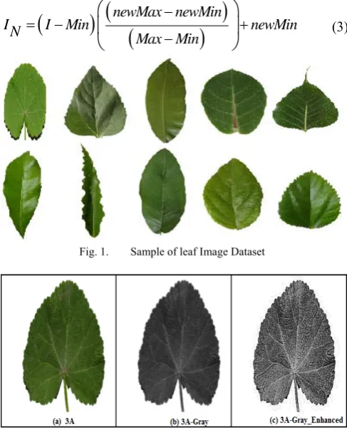
For the experimental research work, a dataset of ten leaves of different classes has been taken as shown in Fig. 1 and for each plant species, 25 images were selected and 250 leaf images in totality were selected for carrying out this study. All the colored leaf images were converted to 8-bit Gray scale images and their size was reduced to 256 X 256, which reduced the size of the dataset. The background of all the images were removed to keep the leaf image intact for future processing.
The 8-bit Gray scale images are normalized which involves stretching the image pixel values to cover the entire pixel value range (0-255). The normalization process [5] transforms the Gray scale image I with intensity values
in the range of
Min, ...,Max
as shown in Eq. (1)
: n , ...,
to a new image IN with intensity values in the range of
newMin,...,newMax
is shown in Eq. (2)
: n ,...,
IN newMin newMax (2)
The linear normalization process is represented with the Eq. (3)
newMax newMin
IN I Min newMin
Max Min
(3)Fig. 1. Sample of leaf Image Dataset
Fig. 2. Leaf image of (a) a colored Slice 3A (b) 8-bit Gray scale Slice 3A (c) 8-bit Gray scale enhanced Slice 3A
Fig. 3. Histogram of leaf image of (a) bit Gray scale Slice 3A (b) 8-bit Gray scale enhanced Slice 3A
Now this IN image undergoes histogram equalization process [6] which is a technique for adjusting image intensities to enhance contrast of the images and this gives image g (a histogram equalized image) which is
represented through the Eq. (4).
1
,, 0
Ii j
gi j floor Max IN
n
(4)Now this gi j, is utilized for further processing and texture features have been extracted.
The original leaf image with its bit Gray scale and 8-bit Gray scale with enhancement is shown in Fig. 2 (a), (b), (c) for Slice 3A respectively. The Histogram is calculated for of 8-bit Gray scale Slice 3A and its enhancement is shown in the Fig. 3(a) and (b) respectively. It can be clearly seen that after enhancement, the image shows proper distribution of Gray level pixels as shown in Fig. 3(b). This process has been adopted for all the leaf images of the dataset. The Gray scaled images and enhanced Gray scaled images have been further used for texture feature extraction in the next subsection.
B. Application of Gray Level Co-occurrence Matrix at different pixel distances
The term texture refers to a feeling of touch which is expected to be rough, smooth or bumpy etc. A rough surface has difference between the high and the low points whereas the smooth surface has its highs and lows of the same value. Therefore, in the case of images the term texture refers to the level of brightness which is expressed as the different values of Gray levels and is expressed in digital numbers. The value of texture quantifies the images and this value expresses the Gray level differences in the images which are called contrast features within a specified size of area of image called window. A brodatz texture [7] images have been shown in the Fig. 4 which represents a very popular texture based dataset.
Fig. 4. Brodatz texture sample
1) Contrast(F1): Contrast is the square of the variance
in the image and is represented through Eq. (5).
1 2
, , 0
N
Contrast Pi j i j i j
(5)
Where , 1, , , 0
vi j Pi j n
vi j i j
Here, in Eq. (5),
P
i j, is the normalization of the Gray value for each cell andv
i j, is the Gray value of each pixel.2) Inertia (F2) and Entropy (F3): It is used for
measuring the disorderliness in a system.
1 2
, ,
N
Inertia Pi j i j i j
(6)
1
( lnP ) , , ,
N
Entropy Pi j i j i j
(7) The term entropy is opposite to that of energy, entropy is a measure for disorderliness and energy is for orderliness and the same has been shown in Eq. (7).
3) Shade(F4): It is the measure of skewness of the
matrix and it measures the perceptual uniformity. When the value of shade is high, the image is asymmetrical. It creates a new image having the range 2(N-1) as shown in Eq. (8).
1 3 , , 0 1 3 , , 02
2
Ni i i j
i j N
j j i j
i j
Shade
i
j
P
Shade
i
j
P
(8)4) GLCM Correlation (F5): The GLCM Correlation
is calculated by using Eq. (9).
1 ,
2
2
, 0
i j
N i j
CORRglcm Pi j
i j i j
(9) With this formula, the correlation between the reference and its neighboring pixel is found out. Here2
i
and
2j are the values of variance.5) Homogeneity (F6) and Inverse Difference Moment (F7): The term homogeneity is calculated using Eq.
(10).
1 , 2
, 0 1 (i j) P
N i j
Homogeneity i j
(10)
Here,
P
i j, , is the normalization of the Gray value for each cell. IDM measures the local homogeneity of theimage. Therefore, for homogenous pixels or near homogeneous pixels, the value for IDM is higher and lower for nonhomogeneous pixels.
6) Angular Second Moment (F8): ASM takes up
square of the normalized value of the Gray level. When the window is orderly, which means similar valued pixels are the nearest neighbors in the window, the ASM value increases and when the window is less orderly, then the value is small and is represented through the Eq. (11).
1 2 , , 0 N ASM Pi j
i j
(11) 7) Energy (F9): It is the square root of the Angular
Second Moment. The ASM and Energy values will be one if all the pixels are the same and the same has been represented through Eq. (12).
1 2 , , 0 N
Energy ASM Pi j
i j
(12) 8) Prominence (F10): It measures the asymmetry in
the image. When the prominence value is high, the image is less symmetric. In addition, when cluster prominence value is low, there is a peak in the GLCM matrix around the mean values and the same has been represented through Eq. (13).
1 4
Prominence 2 ,
, 0
4 1
Prominence 2 ,
, 0 N
i j P
i i i j
i j
N
i j P
j j i j
i j (13)
9) GLCM Variance (F11): The GLCM means can be
derived by using Eq. (14).
1 (P, ) , 0
1 (P, ) , 0 N
i
i i j
i j
N j
j i j i j
(14)
The above equations are the same, but it depends upon whether th
i
orj
thpixel is chosen for calculation purpose. For a symmetrical Gray Level Co-occurrence Matrix, since each pixel becomes neighbor and reference, therefore the value is the same. The variance is a measure of the dispersion of the values around the mean. It is similar to entropy. GLCM Variance in texture measures performs the same task as does the common descriptive statistic called variance. However, GLCM variance uses the GLCM, therefore it deals specifically with the dispersion around the mean of combinations of reference and neighbor pixels, so it is not the same as the simple variance of Gray levels in the original image.1
2 2
(i ) , , 0
1
2 2
(j ) , , 0 N
P
i i j i
i j
N P
j i j i j j
(15)
All the above calculated Gray level co-occurrence features have been computed for both the normal Gray scaled images as well that of the enhanced Gray scaled images for which the contrast values have been improved.
For batch processing, the Gray stacks of the slices of the leaf images are processed through the texture extraction techniques given by [2] which provides the probability of Gray level i occurring in the neighborhood of Gray level j,
given distance d and angle ϴ and total number of Gray
levels N (in the present case 256). The Gray level co-occurrence matrix GM can be expressed mathematically as
follows:
GM Pr( , | , , )i j d N (16)
In order to reduce the complexity, the inter pixel distance
d is kept unity. Normally, in the case of Gray level
co-occurrence matrix based methods, the calculations for feature extraction are carried out at unit pixel distance with
ϴ =0° and 45°, but this work has gone further in extracting the image texture features of the leaf images using Gray level co-occurrence matrix based method at one to five unit pixel distances with angular pixel positions at ϴ =0°, 45°, 90° and 135° independently and then combining them together using ImageJ [8] software. The remaining angular positions of 225°, 270° and 315° are just the mirror images, therefore are not considered.
The texture features dataset at the angular pixel position
ϴ is represented in Eq. (17).
1 2, , ..., 11
TFD F F F (17)
HereF F1 2, , ...,F11 indicate that all the 11 different values
of texture features (mentioned above) measured at a particular value of ϴ which is one of the values of 0°, 45°, 90° and 135°.
The image texture features have been extracted using Co-occurrence matrices with variable pixel distance and variable values for angular positions of the pixels. In this study, the inter pixel distance (k) has been varied from unit
pixel distance to five unit pixel distances and different orientation values of ϴ are 0°, 45°, 90° and 135°. For k=i, where i=1,..,5 the 11 texture features were combined for different values of ϴ. Therefore, for every ki, 11 texture
feature values were calculated for every value of ϴ. The above mentioned methodology was applied to both kinds of images i.e. normal Gray images and enhanced Gray images. For every values of k, for normal Gray images and
enhanced Gray images, the 11 features were combined and finally ten datasets were prepared(5 each for normal Gray and enhanced Gray images) at k=1,2,3,4,5 respectively. The following texture feature datasets have been prepared in this study: Image Texture Dataset Normal Gray (ITDNG),
and Image Texture Dataset Enhanced Gray (ITDEG), using
the Eq. (18) and (19) for i=1,2,3,4,5 respectively.
0, 0, 0, 0
0 45 90 135
ITD TFD TFD TFD TFD
NG ki (18)
0, 0, 0, 0
0 45 90 135
ITD TFD TFD TFD TFD
EG ki (19)
The datasets prepared above were further used for classification purpose in subsection C.
C. Application of Classification Algorithms
To discriminate the features obtained in subsection B into various classes (using different data sets at pixel distance values from k=1 to k=5), the following four classification algorithms have been used: K-Nearest Neighbor (KNN), J48, Classification and Regression Trees (CART), Random Forest (RF) using “caret” package under RStudio [9].
1) K-Nearest Neighbour (KNN): KNN is a non-parametric
technique, as it does not take into consideration the data distribution. KNN is a lazy learning technique as it takes up all the data, and training period is near minimal. This algorithm is able to deal with continuous and categorical dataset.
2) J48: This algorithm is a Java language based
implementation of the C4.5 algorithm of Weka data mining tool. It was developed by Ross Quinlan. This algorithm creates decision trees based on the labelled input data.
3) Classification and Regression Trees (CART):
Classification and regression trees algorithm was given by Breiman Friedman Olsen and Stone. It’s a greedy, top-down binary, recursive partitioning, that divides feature space into sets of disjoint rectangular regions.
4) Random Forest (RF): Random Forest is an ensemble
classifier that consists of many decision trees and outputs the class that is the mode of the class's output by individual trees. Random Forests are often used when we have very large training datasets and a very large number of input variables (hundreds or even thousands of input variables). A Random Forest model is typically made up of tens or hundreds of decision trees.
Each data set was split into two groups (Training and Test sets) in the ratio 75:25. The training data set contains the class labels, whereas the testing dataset does not contain the class labels. The pre-processing of the data involved centring and the scaling of the data matrix. In the classification procedure, a 10-fold cross validation technique has been applied which is repeated three times for validating any predictive model. Predictive accuracy and kappa values have been adopted as a measurable parameter for the classification process. Kappa is defined as the degree of right predictions of a model. This is originally a measure of agreement between two classifiers and is calculated with Eq. (20).
Pr Pr
1 Pr
a e
e
(20)
III.ANALYSIS OF THE RESULTS
The two kinds of datasets (ITDNG and ITDEG) obtained in
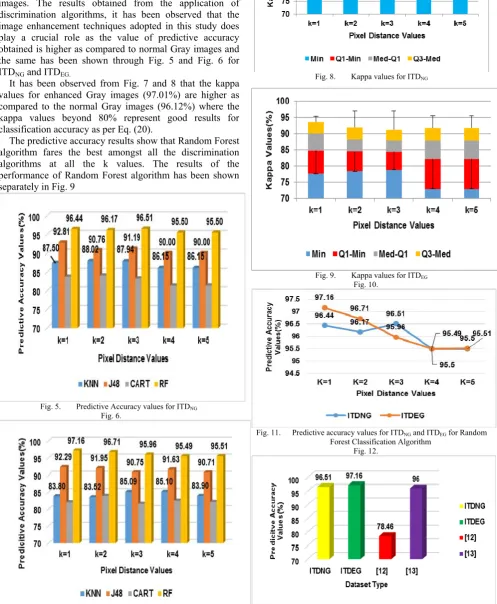
section II were subjected to four discrimination algorithms. For different k values, the highest predictive accuracy value is 96.51% at k=3 for ITDNG. Similarly the highest
predictive accuracy value is 97.16% at k=1 for ITDEG
images. The results obtained from the application of discrimination algorithms, it has been observed that the image enhancement techniques adopted in this study does play a crucial role as the value of predictive accuracy obtained is higher as compared to normal Gray images and the same has been shown through Fig. 5 and Fig. 6 for ITDNG and ITDEG.
It has been observed from Fig. 7 and 8 that the kappa values for enhanced Gray images (97.01%) are higher as compared to the normal Gray images (96.12%) where the kappa values beyond 80% represent good results for classification accuracy as per Eq. (20).
The predictive accuracy results show that Random Forest algorithm fares the best amongst all the discrimination algorithms at all the k values. The results of the performance of Random Forest algorithm has been shown separately in Fig. 9
Fig. 5. Predictive Accuracy values for ITDNG Fig. 6.
Fig. 7. Predictive Accuracy values(in %) for ITDEG
Fig. 8. Kappa values for ITDNG
Fig. 9. Kappa values for ITDEG Fig. 10.
Fig. 11. Predictive accuracy values for ITDNG and ITDEG for Random Forest Classification Algorithm
Fig. 12.
The results obtained in this study have been compared with ([12], [13]). Though the results are not directly comparable due to the different set of leaf images adopted for the preparation of the datasets. The highest classification accuracy achieved in this present study is 97.16% using RF classification algorithm for ITDEG
whereas the maximum predictive accuracy achieved by [12] is 78.46% at unit pixel distance. The maximum accuracy achieved by [13] is 96%. The comparison chart has been shown in Fig. 10, and it has been observed that the enhancement of the leaf images does improve the overall predictive accuracy values.
IV.CONCLUSION
The texture features obtained from the two kinds of datasets shows that the enhancement improves the quality of the leaf images and thereby improving the overall texture feature values. There is a major improvement in the overall predictive accuracy results of enhanced Gray scale images over the normal Gray scale images. As the highest accuracy has been achieved at k=1 for enhanced Gray scale images whereas the highest accuracy in case of normal Gray images was achieved at k=3 and this also reduces the computation time by showing better results at the first computation set. The comparison of the present study with the existing research work proves the objective of the study that image quality does affect the classification accuracy of leaf images.
REFERENCES
[1] Sethulekshmi A.V. and Sreekumar K., “Ayurvedic leaf recognition for plant classification”, International Journal of Comp. Sci. and Info. Tech., vol 5, no. 6, pp. 8061-8066, 2014.
[2] Robert M Haralick , K. Shanmugam and I. Dinestein, “Texture features for image classiifcation”, IEEE Transactions on Systems, Man and Cybernetics, vol. 3, no. 6, pp. 610-621, 1973.
[3] A. Rosenfeld and E. Troy, Visual texture analysis, Computer Sci. Cent., University of MaryLand, College Park, Technical Report, pp. 70-116, 1970.
[4] G. Castellano, L. Bonilha, L.M. Li and F. Cendes, “Texture analysis of medical images”, Clinical Radiology, vol. 59, pp. 1061–1069, 2004.
[5] Webpage on Gabor filter.[Online]. Available: https://en.wikipedia.org/wiki/Gabor_filter
[6] R. C. Gonzalez and R. E. Woods, Digital Image Processing with MATLAB, 2nd Ed., Pearson Education, 2007.
[7] Brodatz database for texture. [Online]. Available: www.ux.uis.no/`tranden/brodatz.html.
[8] Rasband, W.S., ImageJ, U. S. National Institutes of Health, Bethesda, Maryland, USA, 1997-2014.
[9] R Development Core Team, R:A language and environment for statistical computing, R Foundation for Statistical Computing, Vienna, Austria. ISBN 3-900051-07-0., 2008.
[10] Anthony J. Viera, Joanne M. Garrett, “Understanding interobserver agreement:The Kappa statistic”, Family Medicine, vol. 37, no. 5, pp. 360-363, 2015.
[11] Julius Sim , Chris C Wright, “The Kappa statistic in reliability studies: use, interpretation, and sample size requirements”, Physical Therapy, vol. 85, no. 3, pp. 257-268, 2005.
A. Ehsanirad and Sharath Kumar Y.H., “Leaf recognition for plant classification using GLCM and PCA methods”, Oriental Journal of Computer Science & Technology Vol. 3(1), 31-36 (2010)
[12] Li Min., and Jian Jun Liao, ”Texture Image Segmentation Based on GLCM”, Applied Mechanics and Materials, vol. 220-223, pp. 1398-1401, 2012.