Three-State Locally Adaptive Texture Preserving Filter
for Radar and Optical Image Processing
Oleg V. Tsymbal
Kalmykov Center for Radiophysical Sensing of Earth NANU NSAU, 61070 Kharkov, Ukraine Email:[email protected]
Vladimir V. Lukin
Department of Transmitters, Receivers, and Signal Processing, National Aerospace University, 61070 Kharkov, Ukraine Email:[email protected]
Nikolay N. Ponomarenko
Department of Transmitters, Receivers, and Signal Processing, National Aerospace University, 61070 Kharkov, Ukraine Email:[email protected]
Alexander A. Zelensky
Department of Transmitters, Receivers, and Signal Processing, National Aerospace University, 61070 Kharkov, Ukraine Email:[email protected]
Karen O. Egiazarian
Institute of Signal Processing, Tampere University of Technology, 33101 Tampere, Finland Email:[email protected]
Jaakko T. Astola
Institute of Signal Processing, Tampere University of Technology, 33101 Tampere, Finland Email:[email protected]
Received 3 June 2004; Revised 11 October 2004; Recommended for Publication by Moon Gi Kang
Textural features are one of the most important types of useful information contained in images. In practice, these features are commonly masked by noise. Relatively little attention has been paid to texture preserving properties of noise attenuation methods. This stimulates solving the following tasks: (1) to analyze the texture preservation properties of various filters; and (2) to design image processing methods capable to preserve texture features well and to effectively reduce noise. This paper deals with exam-ining texture feature preserving properties of different filters. The study is performed for a set of texture samples and different noise variances. The locally adaptive three-state schemes are proposed for which texture is considered as a particular class. For “detection” of texture regions, several classifiers are proposed and analyzed. As shown, an appropriate trade-offof the designed filter properties is provided. This is demonstrated quantitatively for artificial test images and is confirmed visually for real-life images.
Keywords and phrases:texture feature preservation, image processing.
1. INTRODUCTION
Texture features are widely used in image analysis and recog-nition [1]. This relates to remote sensing applications includ-ing microwave, optical, infrared, and multispectral where texture plays an important role in desired scene-type detec-tion and localizadetec-tion, image classificadetec-tion, object discrimi-nation and terrain delimitation, and so forth [2, 3, 4,5].
imagery the prevailing influence of multiplicative noise is typical and its pdf can be either close to Gaussian or essen-tially non-Gaussian depending upon the radar type and its characteristics [2,5,9,10,11]. This noise is commonly rather intensive and clearly observed visually in microwave images. Noise presence causes problems in information retrieval from grey-scale and color images as well as from radar re-mote sensing data. Noise masks texture, distorts the textural feature parameter estimates obtained from noisy data, makes it more complex to solve the tasks of texture region detection, identification, discrimination, and so forth.
Because of noise, image filtering is a generally used op-eration in remote sensing data processing. It serves the goals of image enhancement, denoising and, as a result, improve-ment of data interpretation, classification, segimprove-mentation, and sensed terrain (scene) parameter estimation [9,10,11]. Al-though a large number of books and papers deal with image filtering, not many of them pay particular attention to tex-ture preservation. To name a few, we mention the papers of Yunhan et al. [10], Aiazzi et al. [12], as well as the book of Perry et al. [13] (see also references therein). Preliminary re-sults of the current paper have been published in [14,15]. The analysis here is more thorough and extended in many respects, one of the most important of which is additionally studied additive noise case.
The paper [10] contains the performance comparison for a rather limited set of filters although it clearly demonstrates the difference in texture preservation for such typical scan-ning window filters as the standard mean and median [8], the local statistic Lee [16], and the sigma [17] filters. The two latter ones are shown [10] to preserve texture well enough. The conclusions given in [10] coincide with the ones pre-sented in our work [14], where the modified sigma filter [18] is also considered.
The paper [12] deals with multitemporal remote sensing data and their applications. Similarly to the data presented in [11,19], Aiazzi et al. underlines that small local variations of true image values that correspond to radar cross-section variations induced by local heterogeneity of surface back-scattering should be preserved after image filtering; and these variations can be considered as texture.
Many other papers relating to image filtering either mainly deal with mosaic images or consider the texture in images under study as edges, details, and their neighbor-hoods (see, e.g., [20,21,22]). Although some concentration of details and some texture can visually have similar appear-ance, they, as it will be shown below, are not the same in the sense of filter performance assessment and filter selection. Si-multaneously, texture and noise are also not the same from the viewpoint of local spatial correlation properties. Perry et al. [13] stress that “the textures usually have noise-like ap-pearance although they are distinctly different from noise in that there exists certain discernible patterns within them.” Here we can also add that while texture contains useful in-formation the noise does not.
Recall that texture features are not the only class of use-ful information to be retrieved from images. For efficient fil-tering, it is also desirable to considerably suppress noise in
image homogeneous (smooth) regions and to preserve edges and details. From these viewpoints, effective image process-ing can be provided by hard-switchprocess-ing locally adaptive filters [20,21,22,23,24]. The simplest versions of such filters that can be referred to as two-component or two-state ones [22] consist of a so-called noise suppressing filter (the standard mean, Wilcoxon, α-trimmed, etc. [8,20,22]) and a detail preserving filter (the local statistic Lee [16], the standard or modified sigma filters [17,18], etc.).
The two-state locally adaptive filter (LAF) output is as-signed to the output of either noise suppressing filter (NSF) or detail preserving filter (DPF). This hard switching is per-formed according to the results of comparing the local activ-ity indicator (LAI) to the predetermined threshold. As LAI, the local statistical parameters like local variance, quasirange, trimmed local variance, and so forth, calculated for given scanning window, are used [20,22]. If the dominant type of noise is multiplicative, then these local statistic parameters are to be normalized [20,22,23].
For two-state LAFs many image texture regions are clas-sified to “locally active areas” and, thus, they are processed by the detail preserving filter (DPF). In general, DPFs [16, 17,18] preserve texture features not badly [10,14]. However, they are not the best choice for processing texture regions. Thus, three problems arise. First, what is the best filter in the sense of texture feature preservation? Second, if there exists such a filter and it is not the same as the best DPF, then, can this filter be incorporated in the structure of the locally adap-tive hard switching filters? The third question is how to detect and localize the texture regions?
In this sense, one should keep in mind that our inten-tion is not to detect one or few particular texture types as in some applications [3,4] but to localize the areas with diff er-ent types of texture characterized by various statistical and/or spatial correlation parameters.
It is worth noting here that more sophisticated versions of locally adaptive filters (with larger number of used com-ponent filters and with more complex methods of analysis of image local behavior) [24,25] are unable to effectively solve the above-mentioned problems since (a) the first question has not been answered there anyway; (b) texture has not been considered as particular class and it could not be so. The rea-son is that image “local analysis” has been performed in the scanning window of size 5×5 pixels [24,25]. At the same time, texture elements generally have larger size and, thus, the sliding windows used in texture analysis and parameter estimation commonly have the size 12×12 or 16×16 pixels [3].
It stems from the theory of hard-switching locally adap-tive filters [20,22,24] that their performance depends upon the selection of component filters. Therefore, for a three-state LAF under design, its performance should depend upon se-lection of NSF, DPF, and texture preserving filter (TPF). The properties of hard-switching LAFs also depend upon the reli-ability of image pixel preclassification, that is, their referring to the corresponding classes.
Such preclassification should successfully solve this task for different levels (variances) and types of noise. We suppose that noise type is either known a priori or predetermined using the corresponding methods, for example, those ones proposed by Carton-Vandecandelaere et al. [26]. Then, the statistical parameters of noise can also be estimated [27,28]. They can be also known a priori. After this, it becomes possi-ble to separately consider the cases of dominant influence of multiplicative or additive noise, and this is done in Sections4 and5, respectively. Numerical simulation data are presented in Sections3,4, and5while real image processing examples are given inSection 6.
2. IMAGE/NOISE MODELS
The noise characteristics of remote sensing (RS) and other kinds of images depend upon different factors [22]. Never-theless, the simplified universal one-channel RS image model can be represented as follows:
Iij= µij·I
true
ij +nij with probability 1−Pimp, Aimp with probabilityPimp,
(1)
whereIijis theijth noisy image sample value,Itrue
ij is the true image value for theijth sample,µij is a stochastic variable that denotes multiplicative noise (withµ = 1 and the rel-ative varianceσ2
µ),nijis the additive noise component with zero mean and varianceσ2
n.Aimpis a value of an image pixel corrupted by impulse spike (or burst) that can be encoun-tered in image sample with probabilityPimp.
Further, we consider impulse-free images since all im-pulse noise and bursts can be removed at the preliminary stage of RS image processing. This can be done using the pre-processing methods proposed by us in [29,30].
As was mentioned in the Introduction, in this paper we consider two basic cases: the dominant influence of multi-plicative (speckle) or additive noise. The situation where an image is corrupted by the former type of noise is considered in this paper in more detail compared to [15].
Multiplicative noise is typical for radar and ultrasound imaging systems [22]. The noise characteristics in radar im-ages depend upon several factors like system type (synthetic aperture radar (SAR) or side look aperture radar (SLAR)) and SAR parameters (one-look or multilook, etc.). The sim-plified radar image models commonly take into account the multiplicative noise only, and can be described as follows [22]:
Iij=Iijtrue·µij. (2)
For the simplified model (2) the influence of radar point spread function and additive noise is neglected. In most real casesµij can be considered as having invariable properties for an entire radar image (σ2
µ =Const). Typical values ofσµ2 are of the order 0.004,. . ., 0.02 for SLAR images and slightly larger for multilook SAR images [22].
The basic attention in this paper is paid to the case when the image is formed by SLAR or by multilook SAR with rather large number of looks. Therefore, it can be supposed that the multiplicative noise pdf is close to Gaussian [22]. However, it is demonstrated inSection 6that the proposed approach is also applicable to processing radar images cor-rupted by nonsymmetric pdf speckle (SARs) if the corre-sponding prefiltering of such images has been carried out.
Another important aspect that we try to stress in this pa-per is the case of prevailing additive noise. For example, for a wide class of optical images the simplified observation model is [8]
Iij=Iijtrue+nij. (3)
Additive noisenijis supposed Gaussian and this assump-tion is valid for many practical applicaassump-tions [8,9,13]. Also, assume additive noise varianceσ2
nis a constant value for en-tire image (σ2
n=Const).
In our simulations we consider i.i.d. (spatially uncorre-lated) multiplicative and additive noise. Although this is not always true in practice (especially, for radar imaging), this paper is only the first step in design of efficient texture pre-serving techniques and, thus, we restricted ourselves consid-ering i.i.d. noise with planning to study spatially correlated noise cases in future.
3. STUDY OF TEXTURE FEATURE PRESERVATION BY DIFFERENT FILTERS
We first perform property analysis of different filters in the sense of texture preservation. Thorough study of such prop-erties for a very wide variety of filters is impossible because of several reasons. First, texture can be characterized and described in different ways using various sets and combi-nations of parameters [1,31, 32, 33]. Really, many diff er-ent approaches involving random Gaussian and Markov field models, fractals, orthogonal transforms, and so forth, are ap-plied to texture modeling nowadays (see [34] and references therein). Second, while analyzing texture feature preserving performance of filters one should keep in mind what will be the further goal of prefiltered image processing (e.g., texture discrimination, parameter evaluation, etc.) and what tech-nique will be applied. Since we do not know the goal of fur-ther image processing in advance, it has been decided to con-sider several typical characteristics and parameters of diff er-ent texture regions for noise-free images, noisy ones, and the images after filtering.
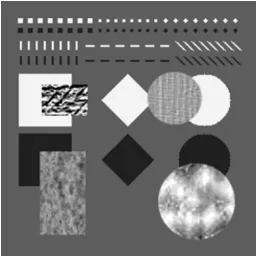
Figure1: The noise-free test image (256×256) with four texture regions.
variance σ2, the skewness ξ, and the kurtosis ψ (nor-malized σ2 was used and it was calculated as σ2 = (1/|Gtext|)ij∈Gtext(Iij−IGtext)
2
/(IGtext)2, whereIGtext denotes the local mean determined for entire texture region Gtext, |Gtext| is the number of pixels that belong to this region). Note that the noise present in an image can rather consid-erably change these statistics in comparison to the noise-free texture (see data presented in Figure 2). Another approach assumes the analysis of spatial spectrum or correlation char-acteristics [1, 5,33] that are connected with cooccurrence matrix-based methods for texture recognition. So, we also consider the basic parameters of spatial autocorrelation func-tion (ACF) like the main lobe width, maximal side lobe level, its visual appearance, and so forth. Besides, some people are more used to analyze the filter performance in terms of mean square error (MSE) or peak signto-noise ratio (PSNR) al-though these are not the best criterions from the viewpoint of processed image quality evaluation [13]. Nevertheless, the integral and local PSNR values have been calculated for en-tire test image inFigure 1and for its fragments.
Analysis has been performed for the four types of tex-ture that had rather different properties. The first texture type is an intensive medium-grain texture (rectangular shape fragment in the left-top part of the test noise-free image in Figure 1, this texture is called “Cement”). The second type called “Linen” is nonintensive small-grain texture (the circu-lar shape fragment in the right-top part). The third sample of texture “Bread” is the large rectangular object in left-bottom part, it can be classified as intensity medium-grain texture. Finally, the fourth texture sample (large-circle shape fragment in the right-bottom part, called “Cracks”) can be classified as medium-intensity large-grain texture. As seen fromFigure 1, beside the aforementioned texture gions (TR), the test image also contains homogeneous re-gions (HR) and edge/detail neighborhood rere-gions (EDNR).
The study of texture feature preserving properties has been performed for a rather wide set of different filters that belong to NSF and DPF classes. As representatives of NSF class, the standard mean (mean), median (median), and the Lpq-NSF also called the sum-rank filter (sum.rank) [22,23] have been exploited. The set of the considered DPFs has in-cluded the following filters. First, the standard sigma (Sigma)
[17], the local statistic Lee (Lee) [16], the center-weighted median (CWMF) [8] with different weights, and the FIR median hybrid filters (modification 3L+ [35]) (FMHF) have been studied. For the two latter filters the scanning window was 5×5, whilst for the standard sigma and Lee filters it var-ied from 3×3 to 9×9 pixels. Second, the modified sigma filters (MSF) have been exploited for the cases of dominant multiplicative [18] and additive [36] noise. Their scanning window size also varied. Besides, for the standard and mod-ified sigma filters as well as for the local statistic Lee filter, we used as the input parameters not only the true values of σ2
µ (orσn2) but also slightly smaller and larger values (they are presented in Table 1). Third, we have also analyzed the filtering method based on spatially invariant discrete cosine transform (DCT) [37,38].
Typically, the transform-based methods are intended for application in additive Gaussian noise environment [37,38, 39]. However, recently there were quite many attempts to modify these methods to make them applicable to process-ing the images corrupted by multiplicative (even speckle) noise [37, 38, 40]. One of the possibilities is to apply at the first stage the direct logarithmic transform Iijh = [alogb(Iij)], whereaandbare some parameters, [·] denotes the rounding-offoperation. Our investigations have shown that if an original radar image is represented as 8-bit 2D data array, the best choice to get 8-bit image representation af-ter direct homomorphic transform and to ensure minimal distortions due to rounding-offerrors is to use a = 8.39 andb = 1.2. Then, the spatially invariant DCT filtering is to be applied followed by the corresponding inverse morphic transform. After the aforementioned direct homo-morphic transform, Gaussian multiplicative noise in original radar image converts to additive quasi-Gaussian noise with varianceσadd2 recalculated asσadd2 =a2σ2
µ/(lnb)2.
The hard-threshold DCT-based filtering presumes assigning zero values to those DCT spectral coefficients that do not exceed the predetermined threshold. This threshold is commonly set proportional to noise standard deviation where the recommendations are to use the factors within the limits from 2 to 4 [39]. According to the results we have obtained by analyzing several textures and noise variances, our recommendation is to set the threshold tDCT twice larger than the noise standard deviation σadd. Note that if the noise in an image is additive, then the operations of direct and inverse homomorphic transform are unnecessary, andtDCT =2σn. The scanning window size for DCT-based filtering was 8×8 pixels although for the 16×16 window the filter performance was almost the same.
Original Noisy Mean Median
Sum. rank Sigma Lee 0.02
0.03 0.04
3 5 7 9
(a)
Original Noisy Mean Median
Sum. rank Sigma Lee
−0.3
−0.2
−0.1 0
3 5 7 9
(b)
Original Noisy Mean Median
Sum. rank Sigma Lee
−0.8
−0.7
−0.6
−0.5
3 5 7 9
(c)
Original Noisy Mean Median
Sum. rank Sigma Lee 0
0.01 0.02
3 5 7 9
(d)
Original Noisy Mean Median
Sum. rank Sigma Lee
−0.7
−0.6
−0.5
−0.4
−0.3
−0.2
−0.1
3 5 7 9
(e)
Original Noisy Mean Median
Sum. rank Sigma Lee
−0.3
−0.2
−0.1 0.1 0.2 0.3
3 5 7 9
(f)
Figure2: Diagrams of statistical characteristics (vertical axis): (a), (d) the relative local variance, (b), (e) the skewness, and (c), (f) the kurtosis of the textural fragment in the right bottom part ((a) , (b), and (c)) and in the left bottom part ((d), (e), and (f)) of the test image
(Figure 1) corrupted by Gaussian multiplicative noise (σ2
µ=0.005) depending on the square sliding window side size (horizontal axis).
Besides, the image texture regions processing by NSF leads to a considerable change in basic characteristics of 2D ACF (compare the ACF inFigure 3ato ACFs in Figures3c, 3d, and3e; also compare the ACF inFigure 4a to the ACF inFigure 4c). In particular, after processing by NSF the ACF main lobe becomes wider; the side lobes are substantially smeared, and so forth. The destructive influence of NSF ap-plication on texture regions will be also clearly seen from the data presented in Table 2 for the 7×7 Lpq-filter where in the rightmost column the values of local MSE and PSNR are given for all texture regions of the test image (in aggregate). Note that all aforementioned effects have been observed for both multiplicative noise variances σ2
µ = 0.005 and σµ2 = 0.012 and for all four considered textures.
In turn, the filters referring to the class of DPFs per-form texture feature preservation much better than any NSF.
After DPF application the valuesσ2,ξ, andψusually become closer to initial values for noise-free texture regions than they were for noisy images. The effect of scanning window size for DPFs is also not as crucial as for NSFs. This is clearly seen for the standard sigma and Lee filters used as examples of DPFs inFigure 2. Besides, as seen in Figures3f,3g, and3h, the 2D ACFs are much closer to the ACF inFigure 3athan the ACFs for outputs of NSFs (Figures3c,3d, and3e). The analysis of 2D ACFs in Figures4dand4ealso shows that they are much more similar to the ACF inFigure 4athan the ACF for the median filter output (Figure 4c).
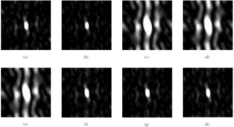
(a) (b) (c) (d)
(e) (f) (g) (h)
Figure3: Two-dimensional grey-scale representation of 64×64 ACFs for the left-bottom texture fragment of (a) the noise-free test image, (b) the test image corrupted by Gaussian multiplicative noise (σ2
µ =0.005), and the same image processed by (c) 7×7 mean, (d) 7×7
median, (e) 7×7Lpq, (f) 7×7 Sigma, (g) 7×7 local statistic Lee, and (h) 8×8 DCT-based filters. (The dynamic diapasons of 2D-ACFs
representation are identically corrected for better visual perception.)
local statistic Lee filter. It is also seen from analysis of ACFs in Figures3hand4fthat the DCT-based filter practically does not distort the 2D ACF of texture samples.
The analysis and comparisons performed above have been done for particular textures and for given values ofσ2
µ. In order to prove that the obtained dependencies and con-clusions are valid for different textures and noise properties, we consider additional simulation data.
As another possible approach, the comparison of texture preserving properties of filters has been also performed using the plots of texture region skewness and kurtosis represented as the corresponding points on plane (seeFigure 5). This fig-ure shows few examples for bothσ2
µ =0.005 andσµ2=0.012 that correspond to typical levels of multiplicative noise in SLAR images.
Numerical results for one more texture sample (right top) that have not been shown inFigure 5can be found in Table 1.
The obtained plots allow to analyze in what degree the skewness and kurtosis are changed after (due to) filtering and to compare the obtained values to original (noise-free) ones. As seen, the considered Lee and DCT filters that belong to DPF class do not change the higher-order statistics too much. For some types of textures practically ideal preservation of texture higher-order statistics is provided by one group of filters. An example is the high-contrast left-top texture (see Figures5cand5f) for which the DCT-based and the 5×5 and 7×7 local statistic Lee produce practically “perfect match.” However, it can be seen that in many cases the FMHF and
sometimes CWMF (with the central weight 11) provide good results as well. Nevertheless, their PSNR results (seeTable 1) are far from the best.
Additional data that characterize texture feature preserv-ing properties of different filters for the four considered tex-ture types are presented inTable 1forσ2
µ =0.005 andσµ2 = 0.012 cases.
As seen, in aggregate, the best results have been provided by the local statistic Lee (5×5 and 7×7) and the proposed version of the DCT-based technique. For them the values of skewness and kurtosis for all four textures differ from the true values by no more than 0.2 (see alsoFigure 5) while for other filters like MSF or CWMF radical changes of these tex-ture featex-tures have been observed. Besides, the Lee and DCT-based filters produce PSNRs that are the largest among all considered filters (i.e., the corresponding values of MSE are the smallest) for all four textures. Note, that the best results are provided by an 8×8 or 9×9 DCT filter. Since the ad-vantage of the latter is not essential, the use of more com-putationally attractive 8×8 DCT variant is preferable. The preponderance of DCT filter is also clearly demonstrated by visual filtering results of texture samples inFigure 6.
0 50 100 150 200 250 300 1 7
13 19 25 31 S1 S11 S21 S31 AC F (a) 0 50 100 150 200 250 300 1 7
13 19 25 31 S1 S11 S21 S31 AC F (b) 0 50 100 150 200 250 300 1 7
13 19 25 31 S1 S11 S21 S31 AC F (c) 0 50 100 150 200 250 300 1 7
13 19 25 31 S1 S11 S21 S31 AC F (d) 0 50 100 150 200 250 300 1 7
13 19 25 31 S1 S11 S21 S31 AC F (e) 0 50 100 150 200 250 300 1 7
13 19 25 31 S1 S11 S21 S31 AC F (f)
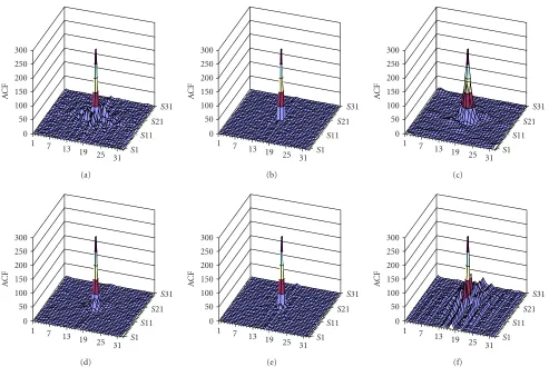
Figure4: Three-dimensional representation of the right-upper texture fragment ACF (32×32): (a) noise-free, (b) corrupted by Gaussian multiplicative noise withσ2
µ=0.012, and after processing the image by (c) the 5×5 median filter, (d) the 5×5 modified sigma filter, (e) the
5×5 local statistic Lee filter, and (f) the 8×8 DCT-based filter.
correspond to noise. Thus, the texture, irrespective of its spa-tial spectral characteristics, is preserved well and noise is ef-fectively suppressed.
The data presented inTable 1one more time underlines the problems of texture region filtering. For some textures like the right-bottom and right-top ones the 4–6 dB PSNR increasing is provided by the best filters and the application of all the considered filters leads to PSNR improving. At the same time, for the left-top texture, practically no improve-ment is ensured even by the best filters. Moreover, the ap-plication of some filters results in even considerable decreas-ing of PSNR. This takes place, for instance, for the CWMF (seeTable 1).
The aggregate PSNR and MSE values calculated for all four texture regions together are given inTable 2in the right-most column. Due to the DCT-based filter application, the PSNR values have been improved (increased) by 4-5 dB. The PSNRs for the DCT-based technique are, at least, by 1−2 dB better than for any other DPF for both σ2
µ = 0.005 and
σ2
µ=0.012.
The final argument that gives additional information to quantitative analysis performed above is visual analysis of texture processing. The visual analysis still remains the key factor from which one can make conclusions concerning
filter quality and conceive the entire explicit numerical re-sults for the considered filters.
The visual results of processing the considered texture samples by some of the studied DPFs are presented in Figure 6. As can be seen, the 5×5 CWMF with the central el-ement weight 11 that provides the best PSNR results among CWMFs does not show good enough texture preservation (Figure 6c); besides, rather intensive residual noise is notice-able. The FMHF that retains high-order statistics well pos-sesses, probably, the worst noise suppression among the stud-ied techniques (see Figure 6d). This fact is also confirmed by the corresponding PSNR values that are rather low (see Table 1). Among sigma filters, the application of MSF even if scanning window is rather small (5×5) results in noticeable detail smearing (Figure 6f) compared to its conventional ver-sion (Figure 6e). For the latter case, noise reduction is not ap-propriate. Nevertheless, fromFigure 6fone can see the MSF tendency to emphasize the edges of small homogeneous ob-ject that is very useful in such class of tasks.
The best overall ability to preserve texture simultaneously with noise suppression is provided by local statistic Lee filter (Figure 6g) and DCT-based filter (Figure 6h).
Noise-free Noisy (0.005) Sigma 5×5 Sigma 7×7 MSF 5×5 MSF 7×7
FMHF
CWMF (w=7) 5×5 CWMF (w=11) 5×5 Lee 5×5
Lee 7×7 DCT 8×8
−0.4
−0.3
−0.2
−0.1 0 0.1
−0.7 −0.5 −0.4 −0.2 −0.1
Ku rt o si s Skewness (a) Noise-free Noisy (0.005) Sigma 5×5 Sigma 7×7 MSF 5×5 MSF 7×7
FMHF
CWMF (w=7) 5×5 CWMF (w=11) 5×5 Lee 5×5
Lee 7×7 DCT 8×8
−1.1
−1
−0.9
−0.8
−0.7
−0.6
−0−.50.1 0 0.1 0.2
Ku rt o si s Skewness (b) Noise-free Noisy (0.005) Sigma 5×5 Sigma 7×7 MSF 5×5 MSF 7×7
FMHF
CWMF (w=7) 5×5 CWMF (w=11) 5×5 Lee 5×5
Lee 7×7 DCT 8×8
−1.3
−1.1
−1
−0.8
−0.7
−0.5
−0.4 −0.3 −0.2 −0.1 0.1
Ku rt o si s Skewness (c) Noise-free Noisy (0.012) Sigma 5×5 Sigma 7×7 MSF 5×5 MSF 7×7
FMHF
CWMF (w=7) 5×5 CWMF (w=11) 5×5 Lee 5×5
Lee 7×7 DCT 8×8
−0.5
−0.3
−0.2 0 0.2 0.3
−0.8 −0.6 −0.4 −0.2 −0.1
Ku rt o si s Skewness (d) Noise-free Noisy (0.012) Sigma 5×5 Sigma 7×7 MSF 5×5 MSF 7×7
FMHF
CWMF (w=7) 5×5 CWMF (w=11) 5×5 Lee 5×5
Lee 7×7 DCT 8×8
−1
−0.9
−0.8
−0.7
−0.60.0 0.1 0.2
Ku rt o si s Skewness (e) Noise-free Noisy (0.012) Sigma 5×5 Sigma 7×7 MSF 5×5 MSF 7×7
FMHF
CWMF (w=7) 5×5 CWMF (w=11) 5×5 Lee 5×5
Lee 7×7 DCT 8×8
−1.3
−1.1
−0.9
−0.7
−0.5
−0.4 −0.3 −0.2 −0.1 0 0.1
Ku rt o si s Skewness (f)
Figure5: Joint graphical representation of kurtosis and skewness for original and noisy textures and these textures are processed by dif-ferent detail preserving filters: (a), (d) left-bottom, (b), (e) right-bottom, and (c), (f) left-top textures inFigure 1, corrupted by Gaussian multiplicative noise: (a), (b), (c) withσ2
µ=0.005 and (d), (e), (f) withσµ2=0.012.
recommended as the best component filter for the three-state locally adaptive hard-switching scheme under design.
As can also be seen from Table 2, the DCT-based fil-tering does not outperform the 7 ×7 Lpq-filter in image homogeneous regions. In turn, the Lpq-filter produces se-vere distortions in texture regions. In edge/detail regions and their neighborhoods the best local MSE and PSNR values are provided by the modified sigma filter. This allows expect-ing that if the image homogeneous regions, the edge/detail neighborhoods, and the texture regions would be reliably classified, the locally adaptive hard-switching filtering could ensure the desirable trade-offof image processing proper-ties.
4. PROPOSED THREE-STATE LOCALLY ADAPTIVE FILTER FOR MULTIPLICATIVE NOISE CASE
Recall that the two-state locally adaptive filter output is de-fined as [20,22,23]
Iijf = INSF
ij , S2 stij =1,
IDPF
ij , S2 stij =2,
S2 st
ij =S1thrij =
1, ϑij≤ϑt,
2, ϑij> ϑt, (4)
where INSF
Table1: Comparative quantitative results of application of different DPFs to four texture samples corrupted by multiplicative Gaussian noise withσ2
µ=0.005 andσµ2=0.012.
Left-top Left-bottom Right-bottom Right-top
texture (Cement) texture (Bread) texture (Cracks) texture (Linen)
PSNR MSE σ2 PSNR MSE σ2 PSNR MSE σ2 PSNR MSE σ2 k γ
Noise-free — — 0.463 — — 0.020 — — 0.027 — — 0.007 0.154 0.236
Noisy (σ2
µ=0.005) 29.01 81.67 0.463 28.47 92.32 0.026 26.09 159.88 0.030 27.2 123.93 0.012 0.259 0.194
Sigma 5×5 28.41 93.89 0.458 29.99 65.13 0.019 28.9 83.75 0.024 29.1 79.93 0.006 0.239 2.293
Sigma 7×7 28.46 92.62 0.457 29.9 66.5 0.018 28.44 93.23 0.023 29.13 79.51 0.005 0.302 2.698
MSF 5×5 26.59 142.5 0.449 29.68 70.09 0.016 29.33 75.86 0.022 28.3 96.29 0.003 0.366 7.728
MSF 7×7 26.98 130.4 0.445 29.58 71.61 0.014 28.5 91.96 0.021 28.49 92.09 0.003 0.717 8.593
FMHF 5×5 24.84 213.4 0.420 29.48 73.36 0.021 27.22 123.42 0.027 28.47 92.79 0.007 0.235 −0.595
CWMF 5×5 (w=7) 15.44 1857 0.224 29.09 80.16 0.013 28.93 83.17 0.021 27.74 109.37 0.002 0.606 0.361
CWMF 5×5 (w=9) 16.94 1315 0.268 29.49 73.07 0.014 28.83 85.15 0.022 28.11 100.58 0.003 0.509 −0.057
CWMF 5×5 (w=11) 18.45 930.2 0.310 29.72 69.33 0.016 28.52 91.41 0.023 28.36 94.91 0.003 0.429 −0.338
Lee 5×5 28.99 82.01 0.452 30.07 64.05 0.020 28.79 85.86 0.025 29.17 78.66 0.006 0.32 0.455
Lee 7×7 28.98 82.27 0.450 29.87 66.96 0.020 28.21 98.16 0.024 29.14 79.21 0.006 0.319 0.422
DCT 7×7 29.02 81.49 0.464 31.4 47.06 0.018 31.98 41.25 0.023 30.82 53.84 0.004 0.316 0.344
DCT 8×8 29.05 81.01 0.463 31.47 46.47 0.018 31.76 43.38 0.023 31 51.63 0.004 0.329 0.193
DCT 9×9 29 81.87 0.464 31.46 48.08 0.018 32.02 40.86 0.024 31.01 51.59 0.004 0.29 0.181
Noisy (σ2
µ=0.012) 25.08 201.9 0.472 24.92 209.6 0.036 22.55 361.3 0.036 23.6 284 0.019 0.329 0.224
Sigma 5×5 24.45 233.2 0.455 27.85 106.8 0.022 26.59 142.8 0.026 26,78 136.5 0.006 0.079 1.625
Sigma 7×7 24.51 230.4 0.451 27.68 111.1 0.020 26.23 155 0.025 26.93 131.8 0.005 −0.036 1.473
MSF 5×5 22.85 337.7 0.440 28.06 101.7 0.015 27.92 104.9 0.022 26.66 140.3 0.002 −0.098 1.762
MSF 7×7 23.04 323.2 0.431 27.75 109.2 0.014 27.05 128.3 0.020 26.99 130.1 0.002 0.158 0.335
FMHF 5×5 23.13 316.6 0.423 26.6 142.2 0.027 24.19 247.8 0.032 25.61 178.8 0.011 0.203 −0.503
CWMF 5×5 (w=7) 15.29 1922 0.220 28.15 99.64 0.015 27.37 119.2 0.024 26.99 130 0.003 0.094 −0.325
CWMF 5×5 (w=9) 16.65 1406 0.264 28.14 99.82 0.017 26.79 136.1 0.025 26.97 130.6 0.004 0.130 −0.469
CWMF 5×5 (w=11) 18.06 1017 0.307 27.94 104.6 0.019 26.15 157.8 0.027 26.78 136.7 0.006 0.169 −0.487
Lee 5×5 25.16 198.2 0.443 28.13 100.1 0.021 27.23 123 0.024 27.24 122.7 0.006 0.423 1.112
Lee 7×7 25.09 201.4 0.439 27.87 106.3 0.020 26.57 143.2 0.023 27.23 123 0.005 0.487 1.049
DCT 7×7 25.14 199 0.471 29.68 69.99 0.017 29.48 73.34 0.023 28.74 86.9 0.003 0.486 0.806
DCT 8×8 25.14 199.3 0.471 29.76 68.70 0.018 29.48 73.26 0.023 28.9 83.7 0.003 0.488 0.729
DCT 9×9 25.16 198.2 0.471 29.68 69.95 0.017 29.65 70.50 0.023 28.99 82.1 0.003 0.389 0.444
corresponds to a locally passive area to be processed by NSF, and ifϑij> ϑt, it belongs to a locally active area to be filtered by DPF.
We now briefly consider the most typical LAIs. For mul-tiplicative noise case they are the relative local variance (RLV) and the normalized quasirange (NQ) [20] derived as follows:
σ2
rij =
i+(N−1)/2
k=i−(N−1)/2
j+(N−1)/2
l=j−(N−1)/2
Ikl−Iij2
m2−1I2
ij ,
Qnij=I
(p)
ij −Iij(q)
I(p)
ij +Iij(q) ,
(5)
whereIij=ik+(=iN−−(N1)−/21)/2
j+(N−1)/2
l=j−(N−1)/2Ikl/m2is the local mean, N =m×mdenotes the scanning window size,Iij(p)andIij(q) are the pth- andqth-order statistics determined for theijth scanning window position,p+q=N+1. In our experiments we usedp≈0.76Nandq≈0.24N.
Numerical simulation results for two versions of the two-state LAF (based on RLV and NQ used as ϑij in (4)) are presented inTable 2(two-state switching scheme). The two component filters (NSF and DPF) were the 7×7Lpq-filter [20,23] (for which the output was calculated asIijLpq =(Iij(p)+ I(q)
(a) (b)
(c) (d)
(e) (f)
(g) (h)
Figure6: Visual representation of filtering results of four texture samples corrupted by (a) multiplicative noiseσ2
µ =0.012, and (b) by
different DPFs: (c) the 5×5 CWMF with the central element weight 11, (d) the FMHF, (e) the 5×5 sigma filter, (f) the 5×5 MSF, (g) the 5×5 local statistic Lee filter, and (h) the 8×8 DCT-based filter.
As seen, the aggregate MSE and PSNR calculated for en-tire image are improved only a little in comparison to the 7×7 modified sigma filter. However, the improvement in image homogeneous regions due to application of the 7×7 Lpq-filter to them is of about 1 dB. The local MSE and PSNR in edge/detail and texture areas are practically the same as for the modified sigma filter since this filter is mostly used for processing the image in these areas.
The output of this two-state LAF applied to the noisy im-age inFigure 7ais presented inFigure 7b. Efficient noise sup-pression in HRs and good edge/detail preservation are ob-served. But the texture in texture regions (TRs) is distorted (compare the images in Figures7band1).
We consider the possibilities to get around these short-comings by developing three-state LAFs. In general, the
three-state locally adaptive filter can be defined as
Iijf =
INSF
ij , S3 stij =1,
IDPF
ij , S3 stij =2,
ITPF
ij , S3 stij =3,
(6)
where now, opposite to (4), the PC (S3 st
ij ) can get three values—1, 2, and 3. The latter corresponds to the case of the given pixel classification as belonging to TR for which the texture preserving filter (TPF) is applied (its output is de-noted asIijTPF).
Table2: Aggregate and local MSE and PSNR values for nonadaptive and locally adaptive filters for the test image inFigure 1containing four texture fragments. The multiplicative Gaussian noise withσ2
µ=0.005 and withσµ2=0.012 has been added to this image (seeFigure 7a).
The component filters for LAF(σ2
µ=0.005)\[σ2µ=0.012]:
Entire image Homogeneousregions Edge
neighborhoods
Texture regions HR—sum-rank filter 7×7 (q=12,p=38);
TR—DCT-filter (tDCT=8)\[tDCT=13];
EDNR—MSF 7×7 (σ2
r =0.005)\[σr2=0.012] PSNR MSE PSNR MSE PSNR MSE PSNR MSE
Corrupted by multiplicative Gaussian noise withσ2
µ=0.005 29.23 77.56 30.05 64.22 29.32 76.02 27.2 123.88
Sum-rank filter 7×7 21.9 419.73 45.84 1.7 18.57 904.7 19.57 717.57
Sigma-filter 7×7 (σ2
r =0.005) 33.9 26.5 37.72 10.99 34.36 23.85 28.98 82.18
Sigma-filter 7×7 (σ2
r =0.007) 34.57 22.69 39.84 6.75 35.1 20.11 29.12 79.61
Sigma-filter 5×5 (σ2
r =0.005) 33.72 27.62 36.94 13.16 34.02 25.8 29.2 78.16
Sigma-filter 5×5 (σ2
r =0.007) 34.48 23.17 38.79 8.59 34.8 21.52 29.46 73.7
Modified sigma-filter 7×7 (σ2
r =0.005) 34.83 21.37 44.16 2.5 35.58 18.01 28.62 89.43
Lee filter 7×7 (σ2
r =0.007) 32.07 40.36 36.56 14.37 30.2 62.09 29.26 77.11
Lee filter 5×5 (σ2
r =0.008) 32.82 33.96 37.18 12.46 31.12 50.25 29.81 67.99
DCT (tDCT=8) 34.3 24.19 41.59 4.51 31.93 41.68 31.16 49.78
2-state switching RLV (ϑt=0.0063) 34.9 21.07 45.69 1.76 35.58 18.01 28.59 89.89
scheme NQ (ϑt=0.07) 34.84 21.33 44.36 2.38 35.57 18.03 28.61 89.51
3-stat
e
sw
it
ching
sc
heme
2-threshold
RLV (ϑt1=0.0068;ϑt2=0.015) 35.45 18.54 45.54 1.82 34.94 20.83 29.84 67.44
NQ (ϑt1=0.07;ϑt2=0.17) 35.01 20.5 45.65 1.77 33.7 27.74 29.99 65.2
Iterative RLV (ϑt1=0.006; [TTR(%)=74%;M=2.6m]) 35.55 18.14 44.77 2.17 33.91 26.41 31 51.69
NQ (ϑt1=0.11; [TTR(%)=61%;M=2.5m]) 36 16.32 45.16 1.98 34.84 21.33 31.01 51.66
CPC1 36.45 14.74 45.37 1.89 35.95 16.51 30.95 52.27
CPC2 36.37 15 45.78 1.72 36.02 16.25 30.72 55.11
Corrupted by multiplicative Gaussian noise withσ2
µ=0.012 25.62 178.39 26.43 147.97 25.69 175.46 23.62 282.74
Sum-rank filter 7×7 22.05 405.27 42.17 3.94 18.8 857.18 19.55 720.8
Sigma-filter 7×7 (σ2
r =0.012) 30.71 55.22 33.75 27.42 30.7 55.35 26.53 144.54
Sigma-filter 7×7 (σ2
r =0.022) 31.81 42.88 37.21 12.36 31.6 45.03 26.78 136.56
Sigma-filter 5×5 (σ2
r =0.012) 30.52 57.72 33.04 32.27 30.51 57.87 26.69 139.4
Sigma-filter 5×5 (σ2
r =0.025) 31.93 41.7 36.6 14.23 31.7 44.01 27.16 125.2
Modified sigma-filter 7×7 (σ2
r =0.012) 32.26 38.64 40.51 5.79 32.16 39.58 26.6 142.43
Lee filter 7×7 (σ2
r =0.017) 29.96 65.7 37.55 11.44 27.32 120.65 27.28 121.65
Lee filter 5×5 (σ2
r =0.018) 30.66 55.9 36.98 13.04 28.33 95.62 27.79 108.06
DCT (tDCT=13) 31.4 47.08 39.31 7.63 28.71 87.57 28.76 86.58
2-state switching RLV (ϑt=0.015) 32.3 38.32 41.34 4.78 32.16 39.55 26.56 143.73
scheme NQ (ϑt=0.12) 32.29 38.41 41.02 5.14 32.16 39.57 26.58 143.09
3-stat
e
sw
it
ching
sc
heme
2-threshold
RLV (ϑt1=0.014;ϑt2=0.036) 32.77 34.37 41.14 5.01 31.7 43.92 27.78 108.32
NQ (ϑt1=0.12;ϑt2=0.3) 32.67 35.14 40.49 5.81 31.37 47.4 28 103.16
Iterative RLV (ϑt1=0.014; [TTR(%)=77%;M=2.6m]) 32.5 36.57 40.59 5.67 30.53 57.54 28.55 90.76
NQ (ϑt1=0.135; [TTR(%)=69%;M=2.6m]) 32.81 34.05 41.29 4.84 31.4 47.13 28.14 99.85
CPC1 32.9 33.36 41.42 4.69 31.29 48.33 28.43 93.31
CPC2 33.44 29.47 41.92 4.18 32.72 34.74 28.15 99.54
texture types can be exploited. Such features can be verbally described as follows. Texture is mostlyslight (not very
inten-sive) spatial variationsof the image true valuesin the regions
of the size not less than ten to ten pixels (although the first
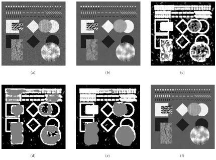
(a) (b) (c)
(d) (e) (f)
Figure7: Examples of the test image (Figure 1) processing: (a) the test image corrupted by multiplicative Gaussian noise withσ2
µ=0.012,
(b) the output of the two-state hard-switching LAF, (c) the result of two-threshold preclassification (7), (d) the “CPC1” classification map, (e) the “CPC2” classification map, and (f) the output of the three-state hard-switching LAF processing according to the CPC2 map.
is present in images, we can also give quantitative definition of texture—for images corrupted by multiplicative noise in texture regions,σ2should be comparable or larger thanσ2
µ. One simple idea [14] is to apply for calculation ofS3 stij = S2 thr
ij the two-threshold scheme like
S2 thr
ij =1 ifϑij≤ϑt1, S2 thr
ij =2 ifϑt1< ϑij≤ϑt2, S2 thr
ij =3 ifϑij> ϑt2,
(7)
whereϑt1andϑt2are the thresholds.
However, the results of such preclassification application are not appropriate [14] since the texture has not been de-tected well enough. As seen inFigure 7c, more than half of the left-bottom texture region is classified as edge/detail ar-eas and intensive texture region (left-top) is fully classified as edge/detail areas; in this map grey color shows detected TRs, black color corresponds to the pixels classified as HR, white ones relate to EDNRs. Other texture regions are also classi-fied not correctly enough. The reason is the empiric selection of the thresholdsϑt1andϑt2. They are set asϑt1≈1.3σµ2and ϑt2≈3σµ2for the RLV (5) used as LAI, andϑt1≈0.05 + 0.6σµ
andϑt2 ≈0.05 + 2σµ for the NQ (5). The drawbacks of this approach to texture detection also deal with the fact that it in no way takes into account the property of texture to occupy rather large spatial areas.
However, even for this, not perfect three-state LAF the aggregate and the local texture MSE and PSNR have im-proved in comparison to the two-state LAF (see the corre-sponding data inTable 2). The basic reason for this is that DCT-based filter has been applied, at least, to some frag-ments of texture regions.
Another proposed method for TR detection and local-ization implies using spatial properties of texture, that is, its property to “cover” some space. For more complicated and efficient PCs with three statesS3 stij we have proposed [14] to apply the iterative approach for which the PC map is formed as
S3 st
ij =
S2t(LAI)
ij , ξijH≤TTR(%),
3, ξijH> TTR(%),
whereξijH=ξ1t(LAI)
ij =
(M−1)/2 k,l=−(M−1)/2
S1t(LAI)
i+k,j+l−1 M2
·100%,
whereξij2t(LAI)is the two-threshold LAI value (calculated us-ing (5) and (7)),ξijHis the heterogeneity indicator expressed in percent for M×M window. The value ofM in the it-erative procedure (8) should be approximately 2.5 times larger than the scanning window side size m for the ini-tial stage of LAI calculation (5) for whichmwas set equal to 7. TTR(%) is the threshold value of heterogeneity per-centage indicator. As ξijH in case of iterative approach, the one-threshold ξij1t(LAI) was used. It is calculated using one-threshold LAIS1ijt(LAI)(S1ijt(LAI)=1 ifQij > ϑandS1ijt(LAI)=0 ifQij ≤ϑ) inM×M window. As LAI in (8), the same LAI was used, either RLV or NQ. The optimal thresholdTTR(%) was about 60–80%. This simple approach was tested earlier in [14].
The numerical simulation results for this approach are presented in Table 2 and marked as “iterative.” Due to better preclassification of TRs, the three-state LAF perfor-mance has been again improved in comparison to the two-threshold three-state hard-switching LAF. Texture preserva-tion has become almost the same as for the DCT-based fil-ter.
A little bit more complex and efficient approach to form-ing the PC with three states S3 stij for more accurate TR de-tection and localization proposed [15] is to apply the com-bined iterative approach where the PC map{SCmb
ij }is formed as
S3 st
ij =SCmbij =
S2t(RLV)
ij , ξijH≤TTR(%),
3, ξijH> TTR(%),
whereξijH=ξ1t(NQ)
ij =
(M−1)/2 k,l=−(M−1)/2
S1t(NQ)
i+k,j+l−1 M2
·100%.
(9)
As can be seen the fixed scheme of combined exploiting theS2ijt(RLV)(calculated using (5) and (7)) andS1ijt(NQ)(see (7)) is used in this case. Recall that in this caseξij1t(NQ)is calculated for only one threshold (S1ijt(NQ)=1 ifQij> ϑandS1ijt(NQ)=0 if Qij ≤ ϑ). So this PC has got the name of combined PC 1 (CPC1). The recommendation concerningMandTTR(%) values are the same as for iterative procedure (8).
Numerical simulation results for this approach (see Table 2) marked as “CPC1” show noticeable improvement of edge neighborhoods region filtering. However, the misclas-sifications are observed in the areas of many small-sized ob-jects concentration (Figure 7d) and this is the drawback of this preclassification method. This drawback deals with the fact that it is very difficult to discriminate the areas of detail concentration and texture fragments.
To get rid of these drawbacks the combined PC 2 (CPC2) was proposed. This approach assumes using the ξij2t(NQ) as heterogeneity indicatorξijH instead ofξij1t(NQ) used by CPC1.
For CPC2 the parameterξij2t(NQ)is calculated based on two-threshold LAIS2ijt(NQ)as follows:
ξ2t(NQ)
ij =
(M−1)/2 k,l=−(M−1)/2
χij
M2 ·100%,
whereχij=
1, S2ijt(NQ)=3,
0, S2ijt(NQ)=1 or 2.
(10)
The CPC2 permits to avoid misclassifications in places of small detail concentration. CPC2 also better than CPC1 localizes low-contrast textures (compare the classification maps in Figures 7d and 7e). The only drawback of CPC2 is misclassification of very high-contrast texture (left-top) as edge/detail region. Because of noticeable loss of PSNR in this region (actually, the local PSNR for the left-top texture pro-cessing for CPC1 is 29.03 compared to 26.98 for CPC2), the three-state LAF based on CPC2 is characterized by 0.08 dB worse PSNR for entire image than the three-state LAF based on CPC1 (for σ2
µ = 0.005). Nevertheless, since such char-acteristics as very high contrasts are not very typical for tex-tures, we can consider the CPC2 classification as conceptually more correct. Moreover, even despite aforementioned mis-classifications, the three-state LAF based on CPC2 ensures noticeable PNSR increasing compared to that one based on CPC1 in the case of larger multiplicative noise variance (see data inTable 2forσ2
µ =0.012).
For CPC2 we recommend to use the following thresh-olds: for RLV set ϑt1 ≈ 1.3σµ2, ϑt2 ≈ 1.9σµ2; for NQ use
ϑt1 ≈0.05 + 0.9σµ,ϑt2 ≈0.05 + 2.5σµ. The valueMin (9), (10) for CPC2 should be approximately 3 times larger than m; the optimal thresholdTTR(%) is about 45–55%.
(a) (b) (c) (d) (e)
Figure8: The visual results of processing the test image (Figure 1) fragment by component filters and their final nonlinear composition: (a) the test image fragment corrupted by multiplicative Gaussian noise withσ2
µ=0.012, (b) the output of 7×7Lpqfilter, (c) the output of 7×7
MSF filter, (d) the output of 8×8 DCT filter, and (e) the output of the three-state hard-switching LAF.
The full-output test image for the three-state LAF based on CPC2 is presented inFigure 7f. Obviously, the consider-ably better texture preservation is ensured compared to the image inFigure 7b.
5. THREE-STATE LOCALLY ADAPTIVE FILTER FOR ADDITIVE NOISE CASE
We now consider the simulation results obtained for domi-nant influence of additive noise (image model (2)). Two vari-ance values σ2
n = 100 andσn2 = 200 have been considered. For additive noise case, as LAIs we used the local variance and quasirange defined as
σ2
lij=
i+(N−1)/2
k=i−(N−1)/2
j+(N−1)/2
l=j−(N−1)/2
Ikl−Iij2
m2−1 ,
Qlij=Iij(p)−Iij(q),
(11)
whereN=m×m=7×7 and, as in previous experiments, p≈0.76Nandq≈0.24N.
A more narrow set of component filters has been studied, namely the Lpq noise suppressing filter, the standard sigma filter and the MSF for additive noise [36], and the DCT-based filter version for additive noise [38]. Exact values of addi-tive noise variance have been used as input parameters of the standard and modified sigma filters.
As earlier, theLpq-NSF and the MSF [36] have been used as components of two-state hard-switching LAF, the thresh-olds have been set according to recommendations given in [20]. The same filters plus the DCT-based filter have been in the staffof three-state LAF. Besides, below we consider only one, the best, version of preclassifier, namely, the CPC2. The recommended values of the thresholds for additive noise case are the following: for local variance (11) set ϑt1 ≈ 1.7σn2, ϑt2 ≈ 1.9σn2; and for quasirange (11) apply ϑt1 ≈ 2.4σn,
ϑt2≈4.5σn. Other settings of the preclassification algorithm parameters areM≈3m;TTR(%) is about 45–55%.
The obtained simulation data for the test image in Figure 1corrupted by additive noise are presented inTable 3. Its analysis shows that the basic tendencies and dependencies earlier observed for multiplicative noise case (seeSection 4) are the same. Again, the 7×7Lpq-NSF is the best for HR processing while the 7×7 MSF preserves edges and details in the best manner. The DCT-based filtering produces the most efficient processing of TRs although the benefit due to its ap-plication depends upon the texture type.
In turn, the proposed three-state LAF provides the max-imal PSNR for entire image as well as the local PSNRs that are the best or, at least, approach to the best reachable values. Clearly, the three-state LAF outperforms the two-state one, and the basic difference in their performance is observed for texture regions. As the result, the difference of about 1 dB is observed for PSNRs evaluated for entire image.
The test image fragment corrupted by additive noise with σ2
n = 200 is presented in Figure 9a. If DCT-based filtering is applied to entire image, one obtains the image repre-sented in Figure 9b. Similarly to multiplicative noise case (seeFigure 8), the basic drawback of the DCT-based filter is observed in the neighborhoods of high-contrast edges and small-sized objects where ringing artifacts are rather clearly seen. Besides, residual fluctuations are visible in image ho-mogeneous regions. These shortcomings are got around in the case of the three-state LAF application (seeFigure 9c).
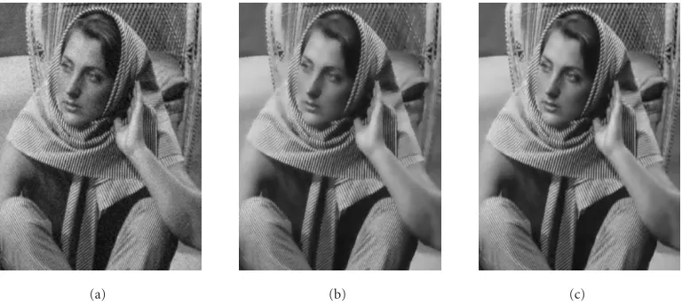
In addition, the simulations for the typical optical test image “Barbara” corrupted by Gaussian additive noise with σ2
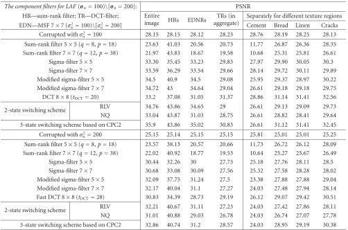
Table3: Aggregate and local PSNR values for nonadaptive and locally adaptive filters for the test image inFigure 1. The additive Gaussian noise withσ2
n=100 and withσn2=200 has been added to this image (Figure 8a).
The component filters for LAF(σn=100)\[σn=200]: PSNR
HR—sum-rank filter; TR—DCT-filter; Entire
image HRs EDNRs
TRs (in aggregate)
Separately for different texture regions EDN—MSF 7×7 (σ2
n=100)\[σn2=200] Cement Bread Linen Cracks
Corrupted withσ2
n=100 28.15 28.15 28.12 28.23 28.76 28.19 28.25 28.13
Sum-rank filter 5×5 (q=8,p=18) 23.63 41.03 20.56 20.73 11.77 26.87 26.36 28.35
Sum-rank filter 7×7 (q=12,p=38) 21.97 43.83 18.67 19.58 10.68 25.31 25.81 26.61
Sigma-filter 5×5 33.30 35.45 33.23 29.83 27.97 29.90 30.05 30.3
Sigma-filter 7×7 33.59 36.29 33.54 29.66 28.14 29.72 30.11 29.89
Modified sigma-filter 5×5 34.5 40.9 34.5 29.08 25.95 29.37 28.97 30.22
Modified sigma-filter 7×7 34.72 43 34.64 29.04 26.61 29.18 29.18 29.75
DCT 8×8 (tDCT=20) 33.2 37.08 31.05 31.37 28.86 31.14 31.41 32.56
2-state switching scheme RLV 34.76 43.86 34.65 29 26.61 29.13 29.09 29.73
NQ 33.04 43.87 31.03 28.75 26.61 28.82 28.41 29.64
3-state switching scheme based on CPC2 35.9 43.86 35.02 30.83 26.61 31.12 31.41 32.45
Corrupted withσ2
n=200 25.15 25.14 25.15 25.15 25.81 25.01 25.01 25.25
Sum-rank filter 5×5 (q=8,p=18) 23.57 38.13 20.57 20.66 11.73 26.72 26.12 28.09
Sum-rank filter 7×7 (q=12,p=38) 22.02 40.92 18.77 19.53 10.64 25.27 25.67 26.49
Sigma-filter 5×5 30.44 32.26 30 27.73 25.18 27.76 28.11 28.5
Sigma-filter 7×7 30.68 33.08 30.09 27.56 25.32 27.58 28.28 28.02
Modified sigma-filter 5×5 32.09 37.75 31.24 27.5 23.38 27.88 27.88 29.04
Modified sigma-filter 7×7 32.17 40.04 31.1 27.27 24.03 27.48 27.94 28.14
Fast DCT 8×8 (tDCT=28) 30.83 34.39 28.73 29.19 26.12 29.07 29.42 30.51
2-state switching scheme RLV 32.21 40.67 31.11 27.23 24.03 27.42 27.86 28.11
NQ 31.01 40.88 29.03 26.78 24.03 26.74 27.07 27.78
3-state switching scheme based on CPC2 32.86 40.74 31.2 28.57 24.03 28.95 29.19 30.38
compared to its two-component predecessor (Figure 10b). The PSNR results show 2.4 dB improvement provided by the two-state LAF and 5.3 dB improvement ensured by the three-state hard-switching LAF. As can also be seen, the residual noise and distortions are practically not seen in the image in Figure 10c.
6. EXAMPLES OF THREE-STATE LAF APPLICATION TO REAL RS IMAGES
The methods of image preclassification and processing based on three-state locally adaptive filtering have been also studied using real-life SLAR and SAR images. An example ofKa-band SLAR image is presented inFigure 11. It has been obtained by airborne radar designed and exploited by the Center of Radiophysical Earth Sensing, Ukrainian National Academy of Science and National Space Agency, Kharkov, Ukraine. For this image, the estimated multiplicative noise variance was 0.005, that is, just like in simulations presented inSection 4.
Comparing the image inFigure 11ato the preclassifica-tion map inFigure 11b, it is seen that the image fragments that either contain obvious texture or do not have very in-tensive local variations of radar cross section are reliably re-ferred to TRs. At the same time, small-sized and prolonged
objects that commonly appear as lighter pixels than the sur-rounding background or are considerably darker like the river in the lower part of the image are also reliably iden-tified as edge/detail neighborhoods and preserved well (see Figure 11c).
The X-band SLAR image formed by aforementioned air-borne multichannel radar complex is shown in Figure 12a. The estimated multiplicative noise variance for this image was 0.012, that is, the same as we used in our simulation experiments (seeSection 4). The modified sigma filter out-put is represented inFigure 12b. Although the noise in HRs is suppressed and the edges and details are preserved well enough, the texture looks smeared and distorted. The three-state LAF has been applied to the original image using CPC2 (Figure 12c), its output is given inFigure 12c. As seen, the texture is preserved better in comparison to MSF while noise suppression and edge-detail preservation are also attained.
(a) (b) (c) Figure9: Visual results of processing the test image corrupted by Gaussian noise withσ2
n=200: (a) original noisy image, (b) the 8×8 DCT
filter output, and (c) the result of image processing by the proposed three-component hard-switching LAF.
(a) (b) (c)
Figure10: Visual results for processing the test image “Barbara” corrupted by (a) Gaussian noise withσ2
n=100 (PSNR=28.12 dB), (b) by
the two-state hard-switching LAF (PSNR=30.58 dB), and (c) by the proposed three-component hard-switching LAF (PSNR=33.43 dB).
results in residual speckle normalization and this is put be-hind the idea to further use the filtering techniques suited to Gaussian noise pdf.
An airborneL-band SAR image withσ2
µ ≈ 0.15 is rep-resented inFigure 13a. Obviously, it is severely degraded by speckle. All the output images (Figures 13b,13c, and 13d) are obtained by means of filtering procedures that presume the aforementioned speckle normalizing preprocessing stage. The final output images after filtering by the 7×7 MSF and the two-state LAF are depicted in Figures 13band13c, re-spectively. As can be seen, speckle is considerably reduced but detail and texture information in most cases is lost. The output of the two-state LAF (Figure 13c) is also very similar to MSF output due to preprocessing phase and using MSF as component filter in LAF. The only difference between the
MSF and two-state LAF outputs is that in latter case more details are lost due to misclassifying of small contrast details to homogeneous regions. At the same time, inFigure 13done can see that the use of the proposed three-state LAF allows us to resolve the task of noise suppression and simultaneous in-formation preservation in a rather good manner even in so complex noise situation.
7. CONCLUSIONS
(a) (b) (c)
Figure11: Visual example of theKa-band SLAR image processing (σµ2≈0.005): (a) the original image, (b) the PC map obtained by CPC2,
and (c) the output of the proposed three-state LAF.
(a) (b)
(c) (d)
Figure12: Visual example of SLAR image processing: (a) the original image, (b) the output of 7×7 MSF, (c) the PC map obtained by CPC2, and (d) the output of the proposed three-state LAF.
have been also taken into account. The study has been per-formed for four textures that considerably differed from each other. As for the result, we have shown that some filters that can be characterized as noise suppressing severely degrade texture. Among the filters that belong to detail preserving class the DCT-based filter has been found the best.
(a) (b)
(c) (d)
Figure13: Real SAR image processing example: (a) the original L-band SAR image, (b) the output of MSF 7×7, (c) the output of two-component hard-switching LAF, and (d) the output of three-two-component hard-switching LAF. All filtering is performed implying prepro-cessing stage (seeSection 6) for speckle normalization.
The reached PSNR improvement is about or more than 1– 3 dB. This benefit is gained due to better texture preservation. The applicability of the three-state LAFs is demonstrated for the real-life SLAR and SAR images. One optical grey scale image processing example is also given.
ACKNOWLEDGMENT
This work has been partly supported by the STCU Grant 1659.
REFERENCES
[1] R. M. Haralick, K. Shanmugam, and I. Dinstein, “Textural features for image classification,”IEEE Trans. Syst., Man, Cy-bern., vol. 3, no. 6, pp. 610–621, 1973.
[2] M. Datcu, D. Luca, and K. Seidel, “Multiresolution analy-sis of SAR images,” inProc. European Conference on Synthetic Aperture Radar (EUSAR ’96), pp. 375–378, Konigswinter, Ger-many, March 1996.
[3] H. Singh and A. Mahalanobis, “Correlation filters for texture recognition and applications to terrain-delimitation in wide-area surveillance,” inProc. IEEE Int. Conf. Acoustics, Speech, Signal Processing (ICASSP ’94), vol. 5, pp. V/153–V/156, Ade-laide, SA, Australia, April 1994.
[4] D. Blacknell and R. G. White, “A comparison of neural net-work and classical texture analysis,” inIEE Seminar on Tex-ture Analysis in Radar and Sonar, pp. 5/1–5/7, London, UK, November 1993.
[5] A. P. Blake, D. Blacknell, and C. J. Oliver, “Texture simulation and analysis in coherent imagery,” inProc. 5th International Conference on Image Processing and Its Applications, pp. 772– 776, Edinburgh, UK, July 1995.
[6] M. Partio, E. Guldogan, O. Guldogan, and M. Gabbouj, “Ap-plying texture and color features to natural image retrieval,” in
Proc. Finnish Signal Processing Symposium (FINSIG ’03), pp. 199–203, Tampere, Finland, May 2003.
[7] J. C. Devaux, P. Gouton, and F. Truchetet, “Application of the Karhunen-Loeve transform to aerial color image segmen-tation,” inProc. 4th International Conference on Knowledge-Based Intelligent Engineering Systems and Allied Technologies, vol. 1, pp. 373–376, Brighton, UK, August–September 2000. [8] J. Astola and P. Kuosmanen,Fundamentals of Nonlinear
Digi-tal Filtering, CRC Press, Boca Raton, Fla, USA, 1997. [9] J. Xiuping and J. A. Richards, Eds., Remote Sensing Digital
Image Analysis: An Introduction, Springer, Berlin, Germany, 3rd edition, 1999.
[10] D. Yunhan, A. K. Milne, and B. C. Forster, “A review of SAR speckle filters: texture restoration and preservation,” inProc. IEEE International Geoscience and Remote Sensing Symposium (IGARSS ’00), vol. 2, pp. 633–635, Honolulu, Hawaii, USA, July 2000.
[11] V. V. Lukin, J. T. Astola, V. P. Melnik, et al., “Data fusion and processing for airborne multichannel system of radar remote sensing: methodology, stages, and algorithms,” inSensor Fu-sion: Architectures, Algorithms, and Applications IV, vol. 4051 ofSPIE Proceedings, pp. 215–226, Orlando, Fla, USA, April 2000.
[12] B. Aiazzi, L. Alparone, S. Baronti, and R. Carla, “Adaptive texture-preserving filtering of multitemporal ERS-1 SAR im-ages,” inProc. IEEE International Geoscience and Remote Sens-ing Symposium (IGARSS ’97), vol. 4, pp. 2066–2068, Singa-pore, August 1997.
[13] S. W. Perry, H.-S. Wong, and L. Guan, Adaptive Image Pro-cessing: A Computational Intelligence Perspective, CRC Press, Boca Raton, Fla, USA, 2002.