ABSTRACT
SICO, KATHLEEN BEETLE. PMU Data Analysis and Short-term Voltage Stability Assessment. (Under the direction of Dr. Aranya Chakrabortty.)
The number of Phasor Measurement Units (PMUs), also called synchrophasors, located across the country has been growing at an astronomical rate. When coupled with existing
construction and maintenance work these devices are inexpensive to implement and provide
valuable data. Now that the PMU infrastructure is in place, there have been many efforts to optimize the use of this data. Given the amount of data, between 30 to 120 samples per second
from each PMU over several measurements, there is a need to develop innovative ways to process
the data and create useful applications for system planners, operators and protection engineers. Duke Energy has installed 125 PMUs across a portion of its service territory and provided this
data for research by a team with members from Duke Energy, SAS and North Carolina State
University (NCSU). This team is tasked with working through data acquisition, examining data quality, baselining and ultimately exploring possible synchrophasor based applications. This
thesis covers the work completed at NCSU towards this project. First, PMU based applications
that have been covered in recent literature are explored. Next baselining results are reviewed including some baselining around events looking at ranges of voltage magnitude, frequency and
voltage phase angle difference as well as dynamic baselineing, evaluating the slow modes or
frequencies of the system. After the baselining results the application of PMU data in voltage stability assessment is more thoroughly reviewed. Since short-term voltage instability can lead
to collapse in under five seconds it is important to evaluate the predictive nature of these
© Copyright 2014 by Kathleen Beetle Sico
PMU Data Analysis and Short-term Voltage Stability Assessment
by
Kathleen Beetle Sico
A thesis submitted to the Graduate Faculty of North Carolina State University
in partial fulfillment of the requirements for the Degree of
Master of Science
Electrical Engineering
Raleigh, North Carolina
2014
APPROVED BY:
Dr. David Lubkeman Dr. Ning Lu
DEDICATION
I would like to dedicate this thesis to my husband Vince Sico. He is the one who encouraged me to return to school and has provided me with love and support throughout my journey. I
BIOGRAPHY
Kathleen Beetle Sico was born in Los Gatos, California on the 5th of May 1975. She completed high school at Walter Hines Page High School in Greensboro, North Carolina in the Spring of
1994. She went on to pursue a Bachelors of Arts degree in Psychology from the University of California Santa Cruz graduating in 1998. In 2008 she decided to return to school to pursue a
Bachelors of Science degree in Electrical Engineering which turned into the pursuit of a Masters
degree with a focus on power systems at North Carolina State University (NCSU).
In order to get experience and affirm her new career decision Kathleen Sico decided to
enroll in the Cooperative Education Program with Duke Energy starting the Fall of 2011.
During her rotations she worked with Substation Electrical and Control Design, Power Delivery Engineering University and Protection and Controls Engineering. Starting in the Fall of 2013
she has been working on the PMU data analysis project, that is the topic of this thesis, with
Duke Energy, SAS Institute and Dr. Aranya Chakrabortty at NCSU. During the Summer of 2014 she worked on a separate project at Duke Energy’s Energy Control Center (ECC) looking
at angular (transient) stability of generating units for a delayed clearing fault. She has excepted
an offer to work as an Engineer I at the ECC starting in January 2015.
Apart from her school and career, Kathleen has a loving husband that she has been married
to since October 2009. Their life together has been enriched by the birth of their first daughter
ACKNOWLEDGEMENTS
There are several people I would like to acknowledge for their support and/or contributions to this project. First I would like to thank my advisor Dr. Aranya Chakrabortty and my supervisor
at Duke Energy Mr. Tim Bradberry for giving me the opportunity to be involved in this cutting edge research. I am lucky to have had the chance to work with Dr. Chakrabortty, who is at
the forefront of research using WAMS technology. He is also one of the best instructors that
I have had, he enjoys teaching as well as research and I have learned a lot from his courses. Tim Bradberry is a very supportive supervisor who has been flexible and understanding of
the balance between work and life which is important for a new mother. He has provided a
lot of useful feedback and I hope he has found the results of this research effort promising for the incorporation of PMU data at Duke Energy. I would also like to thank Dr. David
Lubkeman and Dr. Ning Lu for being part of my graduate committee. Dr. David Lubkeman is
an incredible instructor and has, what seems to be an infinite amount of knowledge, regarding SCADA systems and communication. Although I have not had the pleasure of taking a course
with Dr. Ning Lu she has background in the research regarding the analysis and modeling of
load behaviors which is an important part of voltage stability assessment.
John O’Connor from Duke Energy has been an integral part of the team providing invaluable
information regarding real system phenomena and specific information regarding Duke Energy.
He is a principle engineer with system planning and is an expert in dynamic stability. John is not only my colleague but a mentor, friend, advocate and source of inspiration. From his help
in teaching me the basics of PSSE and dynamic simulations to the theory behind the results I
was able to build confidence in my findings. I am lucky to have John as part of my team and can only hope to accel as he has in my future career.
I would like to acknowledge the other members of our research team from SAS. Greg Link is
responsible for organizing the team at SAS for this research effort, has a background experience in the utility business and from this has provided many ideas regarding the possible uses of
the PMU data. Brad Klenz is an expert with the analysis of big data from various sources and
has provided the team with some insight to big data and statistics which at times would be overlooked by people with utility experience. His knowledge and creativity have been one of the
biggest assets to our team. Brad and I worked together closely on the decision tree portion of this thesis and I learned a lot from him regarding the creation and results of this tool. I would
like to acknowledge Glenn Lampley for his input to this research effort. With prior utility
experience he was able to share ideas, such as detection of equipment failure as a possible use of the PMU data. Last but not least I would like to acknowledge Dr. Arnie DeCastro from SAS.
evaluated during this research effort.
I would like to thank everyone who gave me support from Duke Energy. Megan Vutsinas was my contact for all of this data analysis and any information we needed regarding the PMUs
on the Duke Energy System. In addition Megan also provided me with resource materials from
current efforts in the analysis and use of PMU data. Brian Moss provided me with the resources that we needed to complete the voltage stability simulations. Evan Phillips and Stephen Shuford
provided support with accessing the PMU data as well as using the EPG tools RTDMS and
PGDA. Linwood Ross verified the PSSE channel file buses and lines matched the location of the PMUs in the voltage sensitive region. Doug Steinback and Scott Nyberg helped me obtain and
understand the equivalent impedance of the transmission corridor used for the PV analysis. In
addition, I would like to thank Sammy Roberts, Daniel Stephens and everybody at the ECC. The wealth of knowledge obtained through my internship at the ECC has helped me better
assess the usefulness of the PMU data in operations.
I would like to thank the FREEDM Center for providing the space and resources for this research effort. Karen Autrey organized our monthly meetings and assisted with technical issues
encountered along the way. Dr. Chakrabortty’s research team provided inspiration and support
during my research as well as providing me feedback for my oral examination. In particular I would like to thank Abhishek Jain who taught me how to use Latex, saving me countless hours
of formatting, and provided encouragement, support and honest feedback.
Finally, I would like to thank my family who has supported me in all my endeavors and
has always encouraged my efforts. My husband and daughter have put up with my stress and
limited amount of time and attention. My husbands parents who have made many trips to our house to watch my daughter and who have helped with many other aspects of day to day life. I
couldn’t have asked for better in-laws, they have been a blessing to have as family. My brother
TABLE OF CONTENTS
List of Tables . . . .viii
List of Figures . . . ix
Chapter 1 Introduction . . . 1
1.1 Synchronized Phasor Measurements . . . 3
1.2 Motivation of the Study . . . 4
1.3 Literature Review . . . 5
1.4 Organization of Thesis . . . 10
Chapter 2 Event Baselining . . . 13
2.1 Overview of the Duke Energy System . . . 13
2.2 Event Baselining - Range of Values . . . 16
2.3 Event Baselining - Dynamic . . . 23
Chapter 3 Voltage Stability Overview . . . 34
3.1 Voltage Stability Literature Review . . . 35
3.1.1 Long-Term Voltage Stability . . . 35
3.1.2 Short-Term Voltage Stability . . . 39
3.2 Techniques for Voltage Stability Analysis Using PMU Data . . . 40
3.2.1 Lyapunov Exponent . . . 41
3.2.2 Decision Tree . . . 42
Chapter 4 Voltage Stability Assessment Using The Lyapunov Exponent . . . . 44
4.1 Lyapunov Exponent Algorithm . . . 44
4.2 Sensitivity Analysis . . . 48
4.3 Lyapunov Exponent Matrix . . . 52
Chapter 5 Voltage Stability Assessment Using The Decision Tree . . . 58
5.1 Simulations . . . 58
5.2 Decision Tree . . . 60
5.2.1 Preliminary Decision Tree . . . 60
5.2.2 Final Decision Tree . . . 64
5.3 PV Curve Analysis . . . 66
Chapter 6 Conclusion and Future Work . . . 71
6.1 Baselining . . . 71
6.2 Voltage Stability . . . 72
6.3 Future Work . . . 74
References. . . 76
LIST OF TABLES
Table 2.1 Baselining Line Loss Events . . . 17
Table 2.2 Voltage Magnitude . . . 19
Table 2.3 Frequency . . . 20
Table 2.4 PMU Pairs . . . 21
Table 2.5 Voltage Phase Angle Difference . . . 25
Table 2.6 Dynamic Baselining Events . . . 30
Table 2.7 PMU A . . . 30
Table 2.8 PMU B . . . 30
Table 2.9 PMU C . . . 31
Table 2.10 PMUD. . . 31
Table 2.11 PMUE . . . 31
Table 2.12 PMUF . . . 31
Table 2.13 PMUG . . . 31
Table 2.14 PMUH . . . 31
Table 2.15 PMUI . . . 32
Table 2.16 PMUJ . . . 32
Table 2.17 PMUL . . . 32
Table 2.18 PMUM . . . 32
Table 2.19 Mode Frequency and Damping . . . 33
Table 3.1 Voltage Collapse Incidents 1995-2009 [1] . . . 36
Table 4.1 LE Event Three Final Margin . . . 47
Table 4.2 Operating Conditions . . . 53
Table 5.1 Event Classification Table . . . 65
Table 5.2 Fit Statistics . . . 66
Table 5.3 Operating Condition Cases and Equivalent Impedance of Corridor . . . 67
Table 5.4 PV Curve Summary . . . 69
LIST OF FIGURES
Figure 1.1 PMUs in the United States (a) 2009 [2] (b) 2012 [2] . . . 2
Figure 1.2 (a) Sinusoidal Waveform [2] (b) Phasor Representation [2] . . . 4
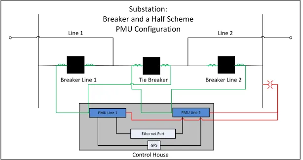
Figure 1.3 PMU Configuration . . . 5
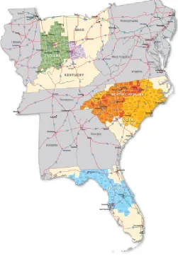
Figure 2.1 Duke Energy Territory . . . 14
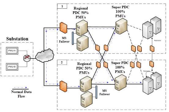
Figure 2.2 PMU Data Flow . . . 15
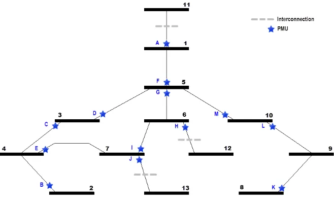
Figure 2.3 500 kV System Model . . . 16
Figure 2.4 PMU I (a) Frequency (b) Voltage Magnitude . . . 18
Figure 2.5 PMU M (a) Frequency (b) Voltage Magnitude . . . 18
Figure 2.6 Voltage Magnitude . . . 19
Figure 2.7 Frequency . . . 20
Figure 2.8 PMU Pairs (a)G-H (b)I-H (c)J-E (d)M-F . . . 24
Figure 2.9 Voltage Phase Angle Difference . . . 25
Figure 2.10 Mode Frequency and Damping Per PMU Per Event . . . 33
Figure 3.1 Impedance Matching Illustration . . . 36
Figure 3.2 Lyapunov Exponent Illustration: Converging and Diverging Trajectories . 42 Figure 4.1 LE (a) PMU B (b) PMUC (c) PMUA (d) PMUL . . . 47
Figure 4.2 IEEE 9 Bus System . . . 48
Figure 4.3 Voltage at Bus 5 during Fault Scenario . . . 50
Figure 4.4 LE Ratio of Neighboring Bus over Faulted Bus . . . 51
Figure 4.5 Voltage Sensitive Region . . . 53
Figure 4.6 Final Margin Generation Loss Event . . . 55
Figure 4.7 Final Margin Line Loss Event . . . 56
Figure 5.1 Preliminary Decision Tree . . . 63
Figure 5.2 PMU Data for Decision Tree Rules Momentary Alarm . . . 63
Figure 5.3 Final Decision Tree . . . 64
Figure 5.4 PV Curve Unity Power Factor . . . 68
Figure 5.5 PV Curve 0.5 Power Factor . . . 68
Figure 5.6 Maximum Power Transfer . . . 69
Figure 5.7 Critical Voltage . . . 69
Figure A.1 LE Generator Loss Event Load Scenario 1 and 2 . . . 84
Figure A.2 LE Generator Loss Event Load Scenario 3 and 4 . . . 85
Figure A.3 LE Line Loss Event Load Scenario 1 and 2 . . . 86
Chapter 1
Introduction
The number of Phasor Measurement Units (PMUs) located across the country has been growing at an astronomical rate as shown in figure 1.1 [2]. Many of these have been installed under
smart grid initiatives of the US Department of Energy (DOE)[3]. When coupled with existing
construction and maintenance work, these devices are inexpensive to implement and provide valuable data.
The PMU, also known as a synchrophasor was introduced in the mid 1980’s and was first
developed at Virginia Tech. Early funding for its development came from the US DOE, the US Electric Power Institute (EPI) and the US National Science Foundation(NSF). The first
installations were in the Bonneville Power Administration (BPA), American Electric Power
(AEP) and New York Power Authority (NYPA) service areas. The PMU combines some of the technology that was introduced in the Symmetrical Component Distance Relay (SCDR) of
the late 1970’s with the synchronized GPS clock signal. The GPS clock can achieve accuracy
of 1 µs which correlates to an angle of 0.021 degrees. The SCDR used a recursive algorithm to calculate the symmetrical components of voltage and current using the Discrete Fourier
Transform (DFT) [4].
Historically the most accurate frequency measurement was at generating stations and re-flected the speed of the rotor which is directly related to the frequency of the generator voltage
(i.e. Watt-Type fly-ball governor of steam turbines). Another method for measuring frequency
is to calculate it from the zero crossings of the voltage. The phasors calculated by the PMU reflect the fundamental frequency component of the voltages and is not affected by
harmon-ics. This technology also extends the frequency measurement to system buses. Power system
frequency measurements are for estimating the rotor speed of the systems generators [5]. The ability for this device to accurately measure phase angle with a synchronized GPS
(a)
(b)
real power flows from large phase angle to small phase angle these measurements can be used to
indicate how the power is flowing across a system. Much of the research that has been conducted on WAMS has focused on using the measurements for monitoring and situational awareness of
large power systems across a large geographical area [3]. Most PMU placement methods focus
on power system observability [6].
1.1
Synchronized Phasor Measurements
Synchronized phasor measurements provide positive sequence voltage and current measure-ments synchronized within 1 µs and local frequency measurements. They can also measure
harmonics , negative sequence, zero sequence and phase voltages [5]. A phasor contains
infor-mation about the magnitude and angle of a sinusoidal waveform. The angle is the deviation from a referenced time or angle as shown in Figure 1.2 [2]. Given the following sinusoidal function
f(t) =V cos(ωt+δ) (1.1)
Using Euler’s formula we can rewrite (1.1).
f(t) =V ∗ e
j(ωt+δ)+e−j(ωt+δ)
2 (1.2)
By extracting the real portion of (1.2) we have
f(t) =Re{V ej(ωt+δ)} (1.3)
Since we know the frequency we can eliminate this term in the shorthand notation of the
phasor expression and write
f(t) =V ejδ =V6 δ (1.4)
Phasor representation is only possible for a pure sinusoid. All signals from the power system
will have components of multiple frequencies. In order obtain a phasor measurement a single frequency needs to be isolated. Ultimately the signal can be expressed as a sum of sinusoids, or
a fourier series, and from this the pure sinusoid at the fundamental frequency can extracted. The Discrete Fourier Transform (DFT)is the process used with sampled data. This process is
explained in detail in [5].
These voltage measurements are taken from the bus potential transformer (PT) or capaci-tance coupled voltage transformer (CCVT) and the current measurements are taken from the
line current transformer (CT) and possibly another shared breaker CT depending on the bus
(a) (b)
Figure 1.2: (a) Sinusoidal Waveform [2] (b) Phasor Representation [2]
measurement would be the addition of the current measured at the line breaker CT and the
current measured at the tie breaker CT. The ratios of these transformers are entered into the settings of the phasor measurement unit so that the actual voltage and current at the bus and
on the line are displayed.
1.2
Motivation of the Study
Since the concept, development, installation and implementation of these devices there are
a few things to consider. The amount of data that is measured and sent to a Phasor Data Concentrator (PDC) at 30 to 120 samples per second from each PMU is far too much for
the operator to make any sense of on a real-time basis. Tools must be created to process the
data and provide useful information to system planners, operators and protection engineers. Ultimately the million dollar question is...“Now that we have all this data, how can we use it
to improve our situational intelligence” [2]?
Duke Energy has installed 125 PMUs across a portion of its territory and has provided this data to a team consisting of members from Duke Energy, SAS and NCSU for research. This
team is tasked with working through data acquisition, examining data quality and data
anal-ysis including baselining and exploring synchrophasor based applications for system planners, operators and protection engineers. With help from our collaborators from SAS institute we
completed the data acquisition, data quality and baselining in the Fall of 2013. In the early
Breaker Line 1 Tie Breaker Breaker Line 2
Line 1 Line 2
PMU Line 1 PMU Line 2
Control House
Ethernet Port
GPS
Substation: Breaker and a Half Scheme
PMU Configuration
Figure 1.3: PMU Configuration
1.3
Literature Review
There is a limited amount of literature surrounding baselining of PMU data. The importance of baselining PMU data is that it can reveal different relationships and insights given the higher
time resolution according to [7]. This article suggests that we need a longer history of PMU data to enable more sophisticated baselining techniques. In [8] offline studies of EMS state-estimator
data and stability simulations coupled with data mining techniques are used in the baselining of
phase angle versus power transfer limits to provide synchrophasor-based situational awareness. Initial research on the possible applications of syncrophasors was conducted by Virgina Tech
and Cornell University through funding from BPA, AEP and NYPA[4]. There are several
appli-cations that are a topic of research in which few have been implemented. Of these appliappli-cations most of them focus on monitoring and situational awareness with a few applications in the
control arena [3]. Possible synchrophasor applications reviewed are listed below.
Phasor state estimation
Dynamic model validation
Dynamic stability assessment and instability detection
Visualization of dynamic attributes
Constructing simplified inter-area models
Protection systems with phasor inputs
Wide Area control with phasor feedback
There are many papers that discuss using PMU measurements either in combination with
SCADA measurements or stand alone for the state estimator. When in combination, the PMU measurements are seen as normal measurements and applied as part of the nonlinear state
estimation. When only PMU measurements are used and the system is fully observable, linear state estimation can be accomplished [9].
The state estimator was developed as a better algorithm for more accurately estimating
the state of the system than the traditional load flow. This algorithm takes a large number of imprecise measurements as inputs and estimates the real and reactive power flowing on the lines
as well as the voltage magnitudes and angles at all the buses. Since the bus voltage magnitudes
and angles determine the system power flows and power injections they are considered the state of the system [5]. Therefore, the PMUs are actually able to measure the states of the
system without estimation at the buses where they are located. The voltage magnitude and
angle at all of the neighboring buses can be calculated using the current magnitude and angle measurements and information on the impedance of the line.
Incorporating PMU measurements with existing SCADA measurements in state estimation
is proposed in [10]. In [11] it was found that adding measurements from PMUs in sufficient numbers increases the efficiency and precision of state estimation. When using a topological
algorithm for state estimation, [12] shows that PMU based algorithms are computationally more
simple, systematic and efficient than conventional ones. There are also many papers that explore methods in determining optimal PMU locations to make the measurement model observable
such as shown in [13].
PMU measurements can be used to validate the dynamic model of a complete system, individual generators, aggregate dynamic loads and Flexible AC Transmission System (FACTS)
devices. Since the sampling rate is high enough to observe post event oscillations this can be
compared to results of dynamic simulations using tools such as Power System Simulator for Engineering (PSSE). In [14] post event analysis using PMU measurements were able to verify
system dynamic simulation studies in the Electric Reliability Council of Texas (ERCOT) and enable them to verify dynamic models of conventional and wind generators. Real-time dynamic
modeling, validation and tuning of a synchronous generator was accomplished using Real Time
Digital Simulator (RTDS), PMU measurements and IEC 61850 communication protocol [15]. There has also been work on model validation of FACTS devices, particularly a Static Var
Static Synchronous Condensor [16].
The area that has received the most attention as far as application development is concerned is dynamic stability assessment and detection. There are three main types of dynamic stability.
First there is small-signal stability which focuses on the slow dynamic inter-area oscillations
remaining bounded. Second there is transient stability also termed ‘first swing’ stability which focuses on the initial swing of a synchronous generators’ rotor angle after a disturbance. Finally
there is voltage stability which is a more localized phenomenon that occurs at load centers in
which the voltage depresses below an acceptable level for an extended period of time.
There have been several papers on using PMU data to assess and detect small-signal stability
which is important for systems with clustered generation and load pockets separated by long
transmission lines. Most of this research has been based on the fact that power system mode shapes can determine the participation of different dynamic components in the low-frequency
inter-area oscillations. These modes are calculated from a linearized dynamic model. Since
large scale accurate dynamic power system models are difficult to obtain, measurement based methods have been receiving a lot of attention since they can be created in real-time with PMU
data. Finding these mode shapes through PMU measurements have the advantage of real-time
applications for small-signal stability [17] and the damping of inter-area oscillations.
In [17] a least squares method is used to estimate modes through an auto-regressive
exoge-nous model. In [18] a recursive method of Prony analysis is used to detect ringdown data using phasor measurements. Ringdown data is the data that results after a large disturbance in which
observable oscillations are present. This data can be used to detect the slow inter-area modes
of a system and therefore assist with small-signal stability [18]. A method using PMU data to monitor the dynamic status of power transfer paths with adapted energy function analysis
is proposed in [19]. This energy can be decomposed into a swing and slow quasi-steady-state
components which can be used to monitor damping and transfer path synchronizing stability respectively. This method is demonstrated on real PMU data from the WECC system which
recorded an event causing 0.578 Hz oscillations along a transfer path 600 miles long from a
median size group of machines supplying power to a remote load center which lasted a total of 5 minutes. In [20] an automated real-time oscillation monitoring system for small-signal
in-stability detection without need for human intervention during analysis is proposed. This is
realized using the classical multi-input Prony algorithm, the matrix Pencil algorithm and the Hankel total least square method. This monitoring tool will issue operator alerts and control
triggers when the damping level of these mode oscillations reach predetermined thresholds. An
added benefit to assessing small-signal stability is the possibility of adding control in the form of inter-area oscillation damping. A method for accomplishing this is proposed in [21] and
con-sists of three steps. First the PMU data is used to identify second order aggregate models for
Second a desired closed loop transient response is achieved between each cluster pair of the
reduced model using state-feedback controllers. Finally an aggregate distributed control design is tuned to realistic generator controls until the response of the real full order system matches
the desired response of the reduced order system.
Normally, transient stability is assessed by looking at the post disturbance values of gener-ator rotor angles. The assessment of transient stability was usually based on offline simulations
using the system model with assumed system conditions and contingencies based on intelligent
decisions made by subject matter experts with knowledge of system vulnerabilities. Since the implementation of WAMS technology there has been research on fast detection of transient
stability using PMU data. Some algorithms have used voltage phase angle and frequency
mea-surements to determine transient stability. One of these algorithms uses the synchronized phase angle to determine if any angle deviation in a particular area start to move away from a center
of inertia reference. Another method approximates the potential and kinetic energy of
genera-tors using voltage phase angle and frequency measurements. An additional algorithm quantifies the stability threshold along system trajectories [22]. In [23] a method using PMU data and
artificial neural networks (ANN) for transient stability prediction in real-time is proposed. This
paper further proposes a transient instability mitigating control scheme that involves inten-tional islanding and initiation of under frequency load shedding. Using the voltage magnitude
at generator buses opposed to rotor angle or frequency in the detection of a power system’s proximity to transient instability is proposed in [24] with a 95 percent success rate. In [25]
a PMU based technique using the Lyapunov Exponent (LE) is proposed and tested. LEs are
used in ergodic theory of dynamical systems to characterize the exponential convergence or divergence of nearby trajectories.
According to IEEE and CIGRE working groups [26] “voltage stability refers to the ability
of a power system to maintain steady voltages at all buses in the system after being subjected to a disturbance from a given initial operating condition.” From [27] “voltage instability stems
from the attempt of load dynamics to restore power consumption beyond the capability of the
combined transmission and generation systems.” Since synchrophasor based applications for the assessment and detection of voltage stability is the focus of our research we have done a
more extensive literature review covered in chapter three.
Creating visualization tools for use in control room applications, which will be the interface between PMU data and system operations, is vital for the optimal use of this data in real-time.
There are numerous displays utilized to manage SCADA measurements and state estimation
that are already implemented in the control room. Most control rooms have approximately six computer monitors per operator but not all of the displays are viewed at the same time. Adding
another display to the mix is something that most system operators are hesitant to accept. This
free and actionable important for acceptance in the control room.
A proposed example of using a contour map with measurements of phase angle differences across a geographical map is discussed in [28]. Electric Power Group (EPG) has created a Real
Time Digital Monitoring System (RTDMS) for use with WAMS technology. It serves as as a tool
to translate research concepts and algorithms for use by system operators, operating engineer support and reliability coordinators. It is an open platform that is scalable with a modular
system design that offers a suite of applications for visualization, monitoring and alarming on
grid stress, dynamics and proximity to instability [29]. This software can be complimented with a post event data analysis tool also produced by EPG called Phasor Grid Dynamic Analyzer
(PGDA). Another tool for visualizing and correlating the dynamic attributes of a system using
PMU data is proposed in [30]. In this visualization tool, mode frequency, damping, residue (participation factor) and mode energy can be visualized on top of a geographical map. Two
types of plot designs are discussed in this thesis: one comprises a set of holistic geospatial
visualizations that includes trends and outliers and the second design supports exploration and further analysis. In another paper [31] a real-time visualization tool using hybrid SCADA and
PMU measurements is proposed. There are several possible display methods that are discussed
including a contour map with colors representing phase angle differences and thermometer type graphics representing voltage magnitude, a grid view with meters showing phase angle
differences, one that highlights rapid changes and one that couples with the contingency analysis tool to show worst-case overloads.
PMU measurements can be used in system identification in which a model is constructed
from a combination of its outputs and possibly some inputs. System identification can be useful when one does not know the precise physical laws governing the system. For this to be realized in
linear time invariant (LTI) discrete time dynamical systems we need to make three assumptions.
The system must be controllable and observable, the input needs to be significant enough to “stir” the contribution of the dominant dynamic modes in the output, and there are no future
inputs or past states that are affecting the output data [32].
In this analysis we assume that the significant input is an impulse and the initial value of the state of the system is zero. Using this to evaluate the general dynamic state space model leads
to a pattern that can be used to develop the Hankel matrix which is realized as the product of
the observability matrix and the controllability matrix.
The method above can be applied to estimate the dynamic model and using the state matrix
we can extract the different mode frequencies of a system as well as their residue (participation
factor) and energy. Power systems are usually divided between fast modes or intra-area modes and slow modes or inter-area modes. These inter-area modes are usually between 0.1 to 1 Hz
in frequency and are prominent in the Western Electric Coordinating Council (WECC).
equivalencing methods are numerically challenging, time consuming and require precise
param-eter knowledge [33]. In [33] this information is used to build a simplified electro-mechanical model of the Pacific AC inter-tie consisting of a three area star connected topology. In another
paper [3] the information was used to create a simplified equivalent five machine inter-area
model of the US west coast grid. One method for identifying the topology for these equivalent models using subspace identification methods is introduced in [34].
There are several applications that use PMU data within protection systems. Traditional
protection is closely related to circuit breaker operation that protects faulty or overloaded equipment, people, animals and property from injury and damage caused by electric faults.
Wide area or system protection is protection that is used to save a system from a blackout or
brown-out situation. In these particular situations there are (not necessarily) individual pieces of equipment that are faulty or overloaded. This can occur when the system is stressed, or
op-erated close to its limits and can actually become worse when traditional protection operates to
clear faulty equipment and lines under stressed conditions [35]. Most of the protection applica-tions using PMU data fall under the umbrella of adaptive protection. Adaptive protection can
use current prevailing power system conditions to change their characteristic where as
tradi-tional protective systems respond in a predetermined manner. Some opportunities for adaptive protection include out of step protection, transformer protection and system restoration. Other
protection schemes that can benefit from phasor measurements include differential transmission line protection and distance relaying for multi-terminal or compensated transmission lines [5].
Most control is closely linked to protection systems, in fact this particular section of power
systems is typically called protection and control. Traditional protection devices control circuit breakers to clear faulty equipment and protect people. In [35] wide-area control is split between
emergency control and normal control. Emergency control describes actions taken to save the
power system. Some of these could be actions like boosting the exciter on a synchronous gen-erator, changing the direction of a high-voltage dc connection or fast valving to counteract
transient stability. Normal control describes actions taken that are preventative, aiming to
ad-just the present and near future operating conditions to maintain stability. These can be either discrete actions such as the operation of a tap changer or shunt device or continuous such as
frequency control and automatic generation control (AGC). The consequence for the failure of
normal control is an increased risk for instability. The consequence for the failure of emergency control is instability. Therefore, the time and reliability response requirements for emergency
control is much higher.
1.4
Organization of Thesis
Chapter 2: Event Baselining
The second chapter presents the baselining results surrounding events. For all of the
event baselining analysis we looked at data collected from the PMUs installed on the
system. First we look at ranges of values for three specific measurements including volt-age magnitude, voltvolt-age phase angle and frequency. Second we explore baselining around
the dynamic slow modes or frequencies of the system using the Eigensystem Realization Algorithm (ERA) implemented in Matlab.
Chapter 3: Voltage Stability Overview
The third chapter covers an extensive literature review of voltage stability assessment
and detection applications using PMU data. From the applications studied we choose
two methods, namely the measurement based LE method and decision tree method, to compare. Since there is no actual PMU data surrounding voltage instability we used Power
System Simulator for Engineering (PSSE) to create simulation data.
Chapter 4: Voltage Stability Assessment Using The Lyapunov Exponent
The fourth chapter covers the measurement based algorithm for calculating the LE, and a couple different techniques using the LE in the assessment and detection of voltage
stability. In one experiment we try to determine if we can calculate the voltage sensitivity
of an unmonitored neighboring bus to a PMU monitored bus as a function of the amount of current on the branch between the two buses. For this analysis we used data from
PSSE simulations of the IEEE 9 bus model. In a second experiment we explore the
relationship between the characteristic of the LE and the final margin as it relates to system contingencies, operating conditions and proximity to voltage stability load limits.
For this analysis we used data from PSSE simulations on Duke Energy’s system model.
Chapter 5: Voltage Stability Assessment Using The Decision Tree
In the fifth chapter we review the efforts between our collaborators at SAS Institute and NCSU in exploring the use of the decision tree data mining technique for the assessment of
voltage stability using the SAS Enterprise Miner software suite. The data that we used to
build the decision tree came from PSSE simulations on Duke Energy’s system model. This chapter reviews the data acquisition process as well as the results from two decision trees.
Finally the subset of the contingencies and operating conditions used in the simulations
are evaluated using the corridor equivalent impedance technique, creating a power versus voltage (PV) curve and calculating the maximum power transfer and critical voltage for
each case.
The sixth chapter summarizes the PMU data analysis covered in this thesis, reviews
the results and draws conclusions based on the results. The first section focuses on the baselining efforts and the second section focuses on the voltage stability assessment. We
propose a syncrophasor application in which the results of this study could be used to
Chapter 2
Event Baselining
2.1
Overview of the Duke Energy System
Today Duke Energy is responsible for providing reliable and affordable electricity to approxi-mately 7.1 million customers over approxiapproxi-mately 104,000 square miles covering six states shown
in Figure 2.1 [36]. Parts of Florida, Indiana, North Carolina, Kentucky, Ohio and South
Car-olina are under the Duke Energy umbrella. In order to cover this load they own approximately 50 GW of net generation capacity provided mostly by hydro, nuclear, coal-fired, combustion
turbine and combined cycle [37]. The Duke Energy territory that this paper is focused on
con-tains approximately 3000 buses with transmission voltages of 500 kV, 230 kV and 100 kV. The Duke Energy owned generation mix includes thirty hydroelectric plants, eight coal-fired steam
plants, four combustion turbine plants and four nuclear plants.
Duke Energy’s vision for synchrophasor technology was developed in the Summer and Fall of 2010 by a team with members from Transmission Planning, System Operations, Telecom,
Energy Management Systems (EMS) Engineering and System Protection. The overall vision requires the integration of synchrophasors into system protection, system planning and system
operations. In the Carolinas the plan was to install up to 104 PMUs at 52 substations providing
100 percent coverage of 500 kV buses, 230 kV buses and 500 kV lines as well as 60 percent of 230 kV lines. In addition to the installation of the PMUs they would need to upgrade substation
communications, upgrade the EMS and install Phasor Data Concentrators (PDCs). Internal and
external subject matter experts determined near term applications which include visualization tools, improved state estimation, system model validation and post event analysis. Longer term
applications would include the monitoring of angular separation and voltage stability margin
[38].
The Duke Energy territory that is the subject of the PMU data analysis in this project
and are also installed on some lower voltage interconnections. Duke Energy is incorporating
EPG’s real-time visualization software RTDMS and post event analysis tool PGDA starting with their operations engineering group. They also plan to update the EMS to a version which
allows the integration of phasors and are looking into gateway devices to exchange data with
external entities.
They have updated much of the substation communication and have installed multiple PDCs
for redundancy. Duke Energy’s PMUs are Schweitzer Engineering Laboratories (SEL) model
351A and have been configured to get 30 samples of data per second. The PDCs are streaming UDP to centrally processed applications using C37.118 protocol. The PMU data flow is shown
in Figure 2.2 [2].
There are 80 TB of storage for PMU data at two different locations. The plan is to have three years of data easily accessible with event data archived for a longer period. There is compression
performed on the most of the data except for frequency which in general is approximately half
the precision of the measuring device. In total there is about 8 GB of data stored per day 3.5 TB per year [2].
Figure 2.2: PMU Data Flow
In the initial stages of the PMU data analysis we wanted to do some baselining around
analyzed ranges of values for frequency, voltage magnitude and voltage phase difference for
each PMU across multiple events. Second we analyzed the dynamic slow frequency modes across multiple events for each PMU. A generic model of the 500 kV system is shown in Figure
2.3.
Figure 2.3: 500 kV System Model
2.2
Event Baselining - Range of Values
For this baselining analysis we obtained four minutes of PMU data, starting at one minute
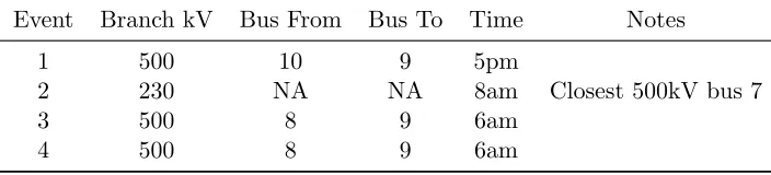
before the event, for the four line loss events from the Fall of 2013 shown in Table 2.1. The
minimum and maximum values of frequency, voltage magnitude and voltage phase difference were evaluated as well as the variance and standard deviation across all events for each PMU.
In order to compare the data from the four events for a single PMU we plotted the different
measurements from 55 seconds to 70 seconds. As expected the PMU closest to the event has the greatest response and the 500 kV PMUs had a greater response from the 500 kV events
than the 230 kV event. In Figure 2.4 we can see that the 230 kV event, event number two, has
Table 2.1: Baselining Line Loss Events
Event Branch kV Bus From Bus To Time Notes
1 500 10 9 5pm
2 230 NA NA 8am Closest 500kV bus 7
3 500 8 9 6am
4 500 8 9 6am
The same is true for the first 500 kV event. This event has the largest response on the graph
for PMU M which is closer to buses 9 and 10 where the line tripped as shown in the following figures. Since PMULgets its data from the line that tripped it did not record data during this
time.
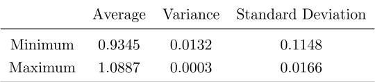
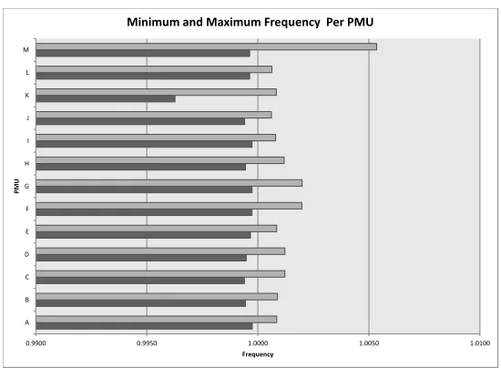
For the voltage magnitude and frequency result summary we converted the values to per unit quantities and plotted the minimum and maximum for each PMU on one chart for voltage
magnitude Figure 2.6 and another chart for frequency Figure 2.7. Next we calculated the average minimum, average maximum, variance and standard deviation across all PMUs. For the voltage
magnitude the average minimum was 0.93 per unit and the average maximum was 1.09 per unit.
(a) (b)
Figure 2.4: PMUI (a) Frequency (b) Voltage Magnitude
(a) (b)
0.50 0.60 0.70 0.80 0.90 1.00 1.10 1.20 1.30 1.40 1.50 A
B C D E F G H I J K L M
Voltage
PM
U
Minimum and Maximum Voltage Per PMU
Figure 2.6: Voltage Magnitude
Table 2.2: Voltage Magnitude
Average Variance Standard Deviation
Minimum 0.9345 0.0132 0.1148
0.9900 0.9950 1.0000 1.0050 1.0100 A
B C D E F G H I J K L M
Frequency
PM
U
Minimum and Maximum Frequency Per PMU
Figure 2.7: Frequency
Table 2.3: Frequency
Average Variance Standard Deviation
Minimum 0.9993 0.000001 0.0009
In order to obtain useful information from the PMU phase measurements we needed to come
up with a reference phase measurement for comparison and compute the difference between the two. Since it makes the most sense to get the phase difference across a single line and none of
the 500 kV lines in the system are tapped we decided to create PMU pairs across each line.
Some of the PMUs were used in more than one PMU pair in order to cover all of the lines. With the exception of two lines and the interconnection points we were able to isolate all of
the lines. Since there is no PMU at bus nine we had to select PMU L and PMU K which is
essentially two lines separated by a bus. Also there is a 500 kV line that goes from one of the buses to a generating station that is not monitored. In total ten PMU pairs shown in Table 2.4
were created.
Table 2.4: PMU Pairs
PMU 1 PMU 2
A F
B E
C E
D G
G H
I H
J E
K L
L F
M F
The phase difference across a line is a strong indication of the real power transfer across that line as shown by the following power transfer equation where real power is traveling from
P = V1V2
X sin(θ1−θ2)
When this quantity is negative it can be interpreted that the real power transfer is from
bus two to bus one. For stability purposes, we want to keep this angle under 90 degrees, where
we hit the maximum power transfer. In the case of a fault we want to make sure that the disturbance doesn’t cause the angle difference to approach instability.
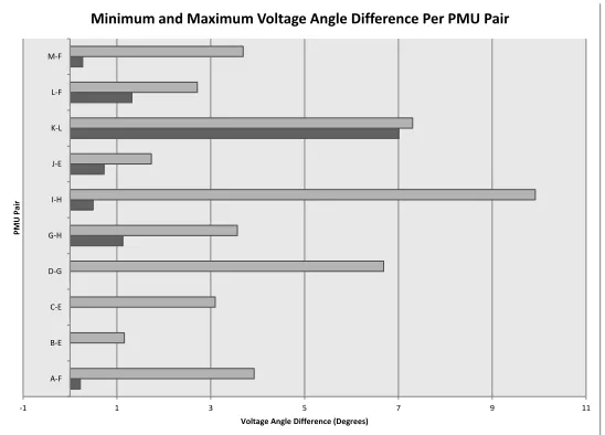
For the four events analyzed the greatest angle difference was approximately 9.92 degrees
between buses I and H during the first event which occurred at 5 pm. One reason for such small angle differences is that these were all events that occurred in the Fall season, or shoulder
month, which is a time where the load (power demand) is minimal. Also, the event that showed
the largest angle difference occurred for an event that was during the daily peak load time frame. For this particular study it appears that the heaviest power transfer is between bus I
and bus H.
However, the flow of power across a power system depends on several factors. Power flow varies with different generation and load patterns, particularly where the generation is coming
from and where the power is being demanded. During a shoulder month power systems complete
most of their construction and maintenance projects which alters the amount and location of generation, transmission and distribution resources. Therefore, it is hard to determine if this
power transfer pattern would be the same for the Summer or Winter months or during a
time when different construction and maintenance projects are taking place. Second, the power transfer across a system depends on the type of load. The difference in the time pattern,
the amount, and the type of power demanded can vary between residential, commercial and
industrial loads. This is due to the fact that commercial and residential loads fluctuate where industrial loads tend to remain constant. This difference is taken into account in planning and
operational studies where the load is incremented. In cases where simulations are performed the industrial load remains constant and the commercial and residential loads are scaled. Third,
the power transfer pattern depends on power transactions between different utilities. Every day
there is power being sold and bought by different utilities in search of the most economical generation to meet their individual loads. These transactions not only affect the systems of the
utilities involved in the ultimate transaction but also affects the utilities in which the power
transverses to get to its final destination. There is little control in the flow of power which is mostly governed by system conditions.
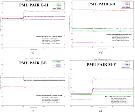
On the other hand there were some interesting observations shown in Figure 2.8. During
the timing of all events it looks like the power flow between some buses were very similar as is shown for PMU pair G to H, bus five to six, and between other buses were very different as
shown for PMU pairI toH, bus seven to six. Similar to the voltage magnitude and frequency,
in the angle difference. For example the PMU pair J toE, bus seven to four, has the largest
response for event two that occurred near bus seven. The PMU pair M toF, bus ten to five, has the largest response for event one that occurred from bus ten to bus nine. Since the PMU
pairs are located on the 500 kV buses there is a larger response seen for the 500 kV events than
the 230 kV event. For the most part the power continued to flow in the same direction except for the case of the PMU pair M toF, ten to five, for event one occurring between bus ten and
nine.
For the result summary we took the absolute value of each phase angle difference in order to evaluate the minimum and maximum quantities. The fact that the angle difference is a negative
quantity indicates the direction of power flow, not the fact that it is smaller than a positive
quantity. After taking the absolute value we plotted the minimum and maximum for each PMU pair on one chart. Next we calculated the average minimum, average maximum, variance and
standard deviation across all PMUs. For the voltage phase angle difference the average minimum
was 1.12 degrees and the average maximum was 4.38 degrees. The standard deviation of these average values is much larger than we saw with voltage magnitude and frequency. This is due
to the nature of the quantity being measured with respect to the power system.
Frequency is the most highly monitored and controlled characteristic of the power system. This is a measure of how well the load and generation are balanced. If the load is greater than
the generation the frequency will fall below 60 Hz. If the generation is greater than the load the frequency will be greater than 60 Hz. Most utilities try to keep this range within 60.05 Hz and
59.95 Hz. Voltage is also a controlled quantity of the power system. Each generator is set up to
control a voltage either at the generator bus on the low side to the step up transformer or at the switchyard bus on the high side of the step up transformer. This is accomplished by adjusting
the excitation of the generator. Voltage regulators, tap changing transformers, capacitor banks
and FACTS devices such as SVCs are all used throughout the system to help maintain an acceptable voltage at every bus. Most utilities try to keep this range between 1.05 per unit and
0.95 per unit. The phase angle difference changes with the power flow on a line. This power flow
can vary significantly depending on load, generation, system configuration and other operating conditions. Therefore it makes sense that we would see a larger standard deviation for the phase
angle difference average values.
2.3
Event Baselining - Dynamic
Next, we wanted to do some dynamic baselining using either the frequency or voltage phase
angle difference characteristic post disturbance to look for slow oscillation modes across the system. This is useful in doing system identification of dynamic models in power systems using
(a) (b)
(c) (d)
-1 1 3 5 7 9 11 A-F
B-E C-E D-G G-H I-H J-E K-L L-F M-F
Voltage Angle Difference (Degrees)
PM
U
Pai
r
Minimum and Maximum Voltage Angle Difference Per PMU Pair
Figure 2.9: Voltage Phase Angle Difference
Table 2.5: Voltage Phase Angle Difference
Average Variance Standard Deviation
Minimum 1.12 4.51 2.12
Realization Algorithm (ERA) implemented in Matlab. This algorithm helps solve a general
subspace ID problem, a powerful tool for constructing discrete-time dynamic models of large order systems in the time-domain using state variable models [39].
Eigensystem Realization Algorithm (ERA) The following explanation describes the
sin-gle input sinsin-gle output (SISO) scenario. The actual ERA allows for the analysis of multiple input multiple output (MIMO) as well. Also, we have used information from [32] to better explain the
following steps. First we assume that the system can be represented by a LTI discrete dynamical
system.
x(k+ 1) =Ax(k) +Bu(k) (2.1)
y(k) =Cx(k) +Du(k) (2.2)
Neither the order of the system or the contents of the matrices (A, B, C, D) above are
known. The measured quantity of frequency or voltage phase angle difference is y(k). The
algorithm conveniently and appropriately assumes the system was excited by a short lived impulse in discrete time. This is appropriate because most large disturbances resemble an
impulse characteristic meaning the disturbance happens at an instant in time and then the
system is left to settle back to an equilibrium without any extended input from the disturbance. Therefore for the input we have the following:
u(k) =
1 fork= 0
0 for all otherk
(2.3)
Another assumption we have to make to complete the algorithm is that there were no initial
conditions, the system was at rest before the input.
x(0) = 0 (2.4)
In order to illustrate the derivation we start by evaluating the state space model at different values ofk.
Iteration 1: k= 0
y(0) =Cx(0) +Du(0)
y(0) =D (2.5)
Iteration 2: k= 1
x(1) =Ax(0) +Bu(0)
y(1) =Cx(1) +Du(1)
from 2.3 and 2.4u(0) = 1, u(1) = 0 andx(0) = 0
x(1) =B (2.6)
y(1) =CB (2.7)
Iteration 3: k= 2
x(2) =Ax(1) +Bu(1)
y(2) =Cx(2) +Du(2)
from 2.3 and 2.6 u(1) = 0, u(2) = 0 andx(1) =B
x(2) =AB (2.8)
y(2) =CAB (2.9)
Iteration 4: k= 3
x(3) =Ax(2) +Bu(2)
y(3) =Cx(3) +Du(3)
from 2.3 and 2.8u(2) = 0, u(3) = 0 andx(2) =AB
y(3) =CA2B (2.11)
From this pattern we can derive the following general equation. These are sometimes referred
to as the Markov Parameters.
y(k) =CAk−1B (2.12)
Using this we can construct a matrix of the output in the following form, known as the Hankel matrix.
H1=
CB CAB CA2B . . . CAM−2B CAM−1B
CAB CA2B CA3B . . . CAM−1B CAMB
..
. ... ... ... ... ...
CAN−1B CANB CAN+1B . . . CAM+N−3B CAM+N−2B
(2.13)
By observation we can see that the structure of this matrix is equal to the product of the
observability and controllability matrices.
H1=OL (2.14)
O=hCT (CA)T (CA2)T . . . (CAN−1)T
iT
(2.15)
L=hB AB A2B . . . AM−1B
i
(2.16)
Next we take the singular value decomposition (SVD) of the Hankel Matrix to eliminate unnecessary modes contained inH1. The ERA prompts the user to enter the number of singular
values that it should use. The SVD is in the following form.
H1 =
h
U1T U2T
i "
Σ1 0
0 Σ2
# "
V1
V2
#
(2.17)
Using the number of singular values the user selects the reduced-order Hankel matrix is in
the following form. Which can be realized as the product of the observability and controllability matrices in a similar manner.
H1=U1TΣ 1 2 1Σ 1 2
1V1 =
h Σ
T 2
1 U1
iT h Σ
1 2
1 V1
i
=OL (2.19)
Next we construct the Hankel matrix starting with the second output as follows.
H2=
CAB CA2B CA3B . . . CAn−1B CAnB
CA2B CA3B CA4B . . . CAnB CAn+1B
..
. ... ... ... ... ...
CAnB CAn+1B CAn+2B . . . CA2n−2B CA2n−1B
(2.20)
From the definitions of the observability and controllability matrices we can rewrite this as
the product of the observability matrix, theA matrix and the controllability matrix.
H2 =OAL=
h Σ
T 2
1 U1
iT A h Σ 1 2
1 V1
i
(2.21)
Since we know what our observability and controllability matrices are as well as the second
Hankel matrix that we derived we can find our A matrix, the state matrix of the system.
A=hΣT2
1 U1
i−T
H2
h Σ
1 2
1 V1
i−1
(2.22)
The eigenvalues of this matrix are responsible for determining the modes of the system.
For the dynamic analysis of the Duke Energy system we collected 15 seconds of data from
19 events. This included 5 seconds pre disturbance and 10 seconds post disturbance. We used
frequency since this measurement produced more pronounced oscillations than voltage phase angle difference. Since the ERA algorithm requires the disturbance to have a certain level of
severity in order to correctly identify the modes we scanned each event for the disturbance
by evaluating the change between samples to be between some range, 1 and 2 . If all of the
PMUs saw the event at the same time we assumed the disturbance was significant enough for
evaluation. If not all of the PMUs saw the event at the same time we did not use the data in our
analysis labeling it as a poorly identified event. Also if the data had data quality issues, such as frequency values that were missing or zero we were unable to use the data. Finally we took
the remaining four events and ran 10 seconds worth of data post disturbance through the ERA program in Matlab, recorded the modes that were less than 1 Hz along with their damping. Of
the four events one was a generation loss event and three were line loss events. The location
Table 2.6: Dynamic Baselining Events
Event Number Event Type kV Bus From Bus To Event Time
1 Line Loss 500 8 9 6am
2 Generation Loss 1pm
3 Line Loss 500 8 9 8pm
4 Line Loss 500 Not Shown 10 10pm
The results are shown below. Although the disturbances for all four events were seen across all of the PMUs there were many data sets that had data quality issues such as missing or
incorrect values for certain PMUs. Therefore, most of the PMUs are missing results for some
of the events.
Table 2.7: PMUA
Event Number Frequency Damping
1 0.6905 0.1864
2 0.6018 0.3040
3 0.4902 0.3787
4
Table 2.8: PMUB
Event Number Frequency Damping
1 0.7153 0.2889
2 0.7921 0.4367
3 0.8451 0.3321
Table 2.9: PMUC
Event Number Frequency Damping
1 0.6538 0.2258
2
3 0.8816 0.2983
4
Table 2.10: PMUD
Event Number Frequency Damping
1 0.6671 0.2202
2
3 0.8576 0.3102
4
Table 2.11: PMUE
Event Number Frequency Damping
1 0.7022 0.2499
2
3 0.8604 0.3385
4
Table 2.12: PMUF
Event Number Frequency Damping
1
2 0.8676 0.4464
3 0.8914 0.2972
4
Table 2.13: PMUG
Event Number Frequency Damping
1
2 0.8730 0.4765
3 0.8765 0.2894
4
Table 2.14: PMUH
Event Number Frequency Damping
1 0.6670 0.2175
2 0.5535 0.6842
3 0.7838 0.3097
Table 2.15: PMUI
Event Number Frequency Damping
1 0.7307 0.3700
2 0.7878 0.3539
3 0.8541 0.2383
4
Table 2.16: PMUJ
Event Number Frequency Damping
1 0.7113 0.3388
2 3
4
Table 2.17: PMUL
Event Number Frequency Damping
1 0.6277 0.1648
2
3 0.6987 0.1912
4
Table 2.18: PMUM
Event Number Frequency Damping
1 0.6275 0.1575
2 0.6134 0.4830
3
4
The following bar chart summarizes the results. Each light grey (frequency) and dark grey
(damping) pair indicate a particular PMU for a particular event. The PMU letter is shown on
the chart and the events are in numerical order according to the events that were evaluated for each PMU which can be determined by looking at Table 2.7 through Table 2.18. The modes
ranged from 0.4902 Hz to 0.8914 Hz with an average of 0.7431 Hz. The median was close to the
average at 0.7230 Hz and the average value had a minimal standard deviation. When rounded to the second decimal place the modes that are repeated the most, three times in the data,
were 0.63 Hz and 0.87 Hz. Although it appears that the results showed modes within a limited
This could be due to the fact that there was not enough good data to evaluate. However, since
slow modes are indicative of oscillations between two areas separated by a long power transfer path and the Eastern Interconnection is a highly meshed system there may not be any easily
defined slow modes.
0.0000 0.1000 0.2000 0.3000 0.4000 0.5000 0.6000 0.7000 0.8000 0.9000 1.0000
A A A B B B B C C D D E E F F G G H H H I I I J L L M M
Fr
e
q
u
e
n
cy
in
Hz
an
d
D
am
p
in
g
525 kV PMU
Modal Analysis Using ERA
Damping Frequency
Figure 2.10: Mode Frequency and Damping Per PMU Per Event
Table 2.19: Mode Frequency and Damping
Minimum Maximum Average Median Variance Standard Deviation
Frequency 0.4902 0.8914 0.7431 0.7230 0.0127 0.1127
Chapter 3
Voltage Stability Overview
There has been increasing focus on the assessment of voltage stability recently. According to IEEE and CIGRE working groups [26] the ability of a power system to maintain an appropriate
steady voltage at all buses after a disturbance is defined as voltage stability. The recent attention
to voltage stability can be attributed to the fact that in the past many utilities invested a large amount in capital, such as generation, transmission and distribution assets, making the system’s
capacity much larger than the demand required. However, as economic pressures have increased,
the trend has changed to a more conservative approach causing the margin between demand and capacity to narrow. From [27] load dynamics attempt to restore power to a load beyond the
capability of the power systems generation, transmission and distribution capacity can result
in voltage instability. Therefore the likelihood of voltage instability has increased.
Power system stability can be divided under two types of classification, first being
generator-driven versus load-generator-driven and second being short-term versus long-term. Voltage stability falls
under both the short-term and long-term load-driven classifications [27]. Long-term voltage stability is a function of the electrical distance between generation and loads which ultimately
depends on the structure of the network at any given time[27]. Long-term voltage stability can
be analyzed using an equivalent impedance and an equivalent generation source voltage at the load bus and calculating the relationship between power and voltage. The most famous form of
this relationship is the real power versus voltage curve also known as the PV curve which can be
realized through the Th´evenin impedance matching technique. The driving force behind long-term voltage instability post contingency is the system’s attempt for load power restoration
such as Load Tap Changers (LTC) coupled with the system’s maximum power being reduced
by generator reactive power limits enforced by Over Excitation Limiters (OEL) [40].
Short-term voltage stability is closely coupled to dynamic load components, mainly
one second [27]. Short-term voltage instability most often results from the fact that induction
motors can stall in reduced voltage scenarios, caused by system disturbances, and under these conditions, can draw up to six times their nominal reactive power [41]. Analysis of short-term
voltage stability is not as straight forward as long-term voltage stability analysis. Not only does
short-term voltage stability assessment rely on system conditions and contingency location but also on accurately modeling aggregate load dynamics. Both long-term and short-term voltage
instability can lead to voltage collapse, where a sequence of events leads to abnormally low
voltage over a large area of the system or a complete blackout [1]. Table 3.1 lists several voltage collapse incidents that occurred between 1995 and 2009.
Another voltage-related phenomenon that can occur is known as Fault Induced Delayed
Voltage Recovery (FIDVR). “FIDVR is a voltage condition initiated by a transmission, sub-transmission, or distribution fault and characterized by the stalling of induction motors, initial
voltage recovery after the clearing of the fault to less than 90 percent of precontingency voltage,
and a slow voltage recovery lasting more than two seconds to expected postcontingency steady-state voltage levels” [1]. If the FIDVR event is severe enough it has the possibility of causing
voltage collapse. Some important factors regarding this phenomenon are (1) the greater the
initial drop in voltage the more reactive power the motor loads demand and (2) the recovery of the voltage depends on the local reactive power support of the system.
3.1
Voltage Stability Literature Review
Our first task is to explore literature on the assessment, detection and control techniques using
PMU data for each of the aforementioned voltage phenomenon. We will start with long-term
voltage stability since this phenomenon has been explored the most in literature. The detection methods for long-term voltage stability using real time measurements have been summarized
and organized in [40]. These methods have been split among methods using wide-area versus
local measurements and non-synchronized (i.e. SCADA) versus synchronized (i.e. PMU) mea-surements. Although this is not an exhaustive list we have used it to organize the following
literature review section for long-term voltage stability. There has been considerably less
liter-ature that consists of using PMU data for the assessment, detection and control of short-term voltage stability.
3.1.1 Long-Term Voltage Stability
Local Measurement Based Methods
There are two main techniques that fall under the category of local measurement based
Table 3.1: Voltage Collapse Incidents 1995-2009 [1]
Date Location Time Frame Load Lost People Affected Cost
11/11/09 Brazil/Paraguay 68 sec 24,731 MW 87 million
6/12/04 Greece 30 min 9.000 MW 5 million
9/23/03 Sweden/Denmark 7 min 6,550 MW 4 million $75 mil 8/14/03 US/Canada 39 min 63,000 MW 50 million $7-10 bil
5/97 Chile 30 min 2,000 MW
8/10/96 Western US 6 min 30,500 MW 7.5 million
6/8/95 Israel 19 min 3,140 MW
be calculated using non-synchronized measurements or synchronized measurements of voltage and current as well as the LIVES technique that uses non-synchronized measurements [40].
Impedance matching is a way of calculating the maximum deliverable power at a load bus.
Given the Th´evenin equivalent of the system at the load bus shown in Figure 3.1 combined with our knowledge from circuit theory the maximum power transfer occurs when the apparent
impedance of the load is equal to the Th´evenin impedance of the system. The LIVES technique attempts to incorporate the effect of the LTC’s attempt to restore load in the assessment of
long-term voltage stability. In our review we will focus on the techniques that use synchronized
measurements specifically impedance matching.
![Figure 1.1:PMUs in the United States (a) 2009 [2] (b) 2012 [2]](https://thumb-us.123doks.com/thumbv2/123dok_us/1642327.1205286/13.612.163.476.74.650/figure-pmus-united-states-b.webp)