Two types of permanence of a stochastic mutualism model

(1)

R E S E A R C H

Open Access

Two types of permanence of a stochastic

mutualism model

Hong Qiu

1,2

_{, Jingliang Lv}

1*

_{and Ke Wang}

1,3

*_{Correspondence:}

[email protected]

1_{Department of Mathematics,}

Harbin Institute of Technology, Weihai, 264209, P.R. China Full list of author information is available at the end of the article

Abstract

A stochastic mutualism model is proposed and investigated in this paper. We show that there is a unique solution to the model for any positive initial value. Moreover, we show that the solution is stochastically bounded, uniformly continuous and globally attractive. Under some conditions, we conclude that the stochastic model is stochastically permanent and persistent in mean. Finally, we introduce some ﬁgures to illustrate our main results.

Keywords: global attractivity; stochastic permanence; persistence in mean; extinction

1 Introduction

Population systems have long been an important theme in mathematical biology due to their universal existence and importance. As far as mutualism system is concerned, lots of proofs have been found in many types of communities. Mutualism occurs when one species provides some beneﬁt in exchange for some beneﬁt. One of the simplest models is the classical Lotka-Volterra two-species mutualism model, which reads

⎧ ⎨ ⎩

dN(t)

dt =N(t)[a–bN(t) +cN(t)], dN(t)

dt =N(t)[a–bN(t) +cN(t)].

()

There are many excellent results on the two-species mutualism model (). It is well known that in nature, with the restriction of resources, it is impossible for one species to survive if its density is too high. Thus the above model is not so good in describing the mutualism of two species (see []). Gopalsamy [] proposed the mutualism model as follows:

⎧ ⎨ ⎩

dN(t)

dt =r(t)N(t)[

K(t)+α(t)N(t)

+N(t) –N(t)],

dN(t)

dt =r(t)N(t)[

K(t)+α(t)N(t)

+N(t) –N(t)],

()

whereN(t) andN(t) denote population densities of each species at timet,ridenotes the intrinsic growth rate of speciesNiandαi>Ki,i= , . The carrying capacity of speciesNiis

Kiin the absence of other species, while with the help of the other species, the carrying ca-pacity becomes (Ki(t) +αi(t)N–i(t))/( +N–i(t)),i= , . It is assumed that the coefficients of the system are all continuous and bounded. Li and Xu [] obtained sufficient conditions for the existence of positive periodic solutions. Chen and You [] gave the sufficient con-ditions for the permanence of the model. Chenet al.[] considered the permanence of a

(2)

delayed discrete mutualism model with feedback controls. Here we transform the system () into the following form:

⎧ ⎨ ⎩

dx(t) dt =x(t)[

a(t)+a(t)y(t)

+y(t) –c(t)x(t)], dy(t)

dt =y(t)[

b(t)+b(t)x(t)

+x(t) –c(t)y(t)].

()

As a matter of fact, population systems are often subject to environmental noise,i.e., due to environmental fluctuations, parameters involved in population models are not absolute constants, and they may fluctuate around some average values. Based on these factors, more and more people began to be concerned about stochastic population systems (see [–]). Especially, Maoet al.[] obtained the interesting and surprising conclusion: even a sufficiently small noise can suppress explosions in population dynamics. Jianget al.[] considered the global stability and stochastic permanence of a stochastic logistic model. Ji

et al.[] discussed the persistence in mean of a predator-prey model with stochastic per-turbation. Now, taking into account the eﬀect of randomly ﬂuctuating environment, we in-corporate white noise in each equation of the system (). Therefore, the non-autonomous stochastic system can be described by the Itô equation

⎧ ⎨ ⎩

dx(t) =x(t)[a(t)+a(t)y(t)

+y(t) –c(t)x(t)]dt+σ(t)x(t)dB(t),

dy(t) =y(t)[b(t)+b(t)x(t)

+x(t) –c(t)y(t)]dt+σ(t)y(t)dB(t),

()

whereai(t),bi(t),ci(t), σi(t),i= ,  are all positive, continuous and bounded functions on [, +∞), andB(t),B(t) are independent Brownian motions,σandσrepresent the intensities of the white noises.

For convenience, iff(t) is a continuous bounded function on [, +∞), we deﬁne

ˆ

f = inf

t∈[,+∞)f(t), ˇ

f = sup

t∈[,+∞)

f(t).

For any sequence{fi(t)}(i= , ) deﬁne

ˆ

f = inf

t∈[,+∞)fi(t), ˇ

f = sup

t∈[,+∞)

fi(t).

To the best of our knowledge, a very little amount of work has been done on the stochas-tic system (). Therefore, we aim to consider dynamical properties of the stochasstochas-tic model () in this paper.

(3)

the system () in Section . We work out some ﬁgures to illustrate the various theorems obtained before in Section . Finally, we close the paper with conclusions in Section . The important contributions of this paper are therefore clear.

2 Basic properties of the solution

2.1 Positive and global solution

Throughout this paper, let (,F,{Ft}t≥,P) be a complete probability space with a ﬁltration {Ft}t≥satisfying the usual conditions. We denote byR+the positive cone inR,X(t) = (x(t),y(t)) and|X(t)|= (x(t) +y(t))_{. And we use}_K_{to denote a positive constant whose}

exact value may be diﬀerent in diﬀerent appearances.

Theorem  For any given initial value X= (x,y)∈R+,there is a unique solution X(t) = (x(t),y(t))to stochastic diﬀerential equation()on t≥and the solution will remain in R +

with probability,that is,X(t) = (x(t),y(t))∈R

+for all t≥almost surely.

Proof The proof is similar to [, ]. Since the coeﬃcients of equation () are locally Lips-chitz continuous, for any given initial valueX∈R+, there is a unique local solutionX(t) ont∈[,τe), whereτe is the explosion time. To show this solution is global, we need to show thatτe= +∞a.s. Letm>  be suﬃciently large forx(t) andy(t) lying within the interval [_m

,m]. For each integerm≥m, deﬁne the stopping time

τm=inf

t∈[,τe) :x(t) ory(t) /∈



m,m

,

where, throughout this paper, we setinf∅=∞. Obviously,τmis increasing asm→ ∞. Let

τ_∞=limm→∞τm, whenceτ∞≤τea.s. If we can show thatτ∞=∞a.s., thenτe=∞a.s. If not, there is∈(, ) andT>  such thatP{τ∞≤T}>. Hence there is an integerm≥m such thatP{τm≤T} ≥for allm≥m. Deﬁne a functionV:R+→R+byV(x) = (x–  –

lnx) + (y–  –lny). The non-negativity of this function can be seen fromu–  –lnu≥ onu> . IfX(t)∈R

+, we obtain that

LV = (x– ) a(t) +a(t)y(t)

 +y(t) –c(t)x(t)

+ (y– ) b(t) +b(t)x(t)

 +x(t) –c(t)y(t)

+σ   +σ



≤(aˇi+cˇi)x(t) –cˆi(t)x(t) + (bˇi+cˇi)y(t) –ˆci(t)y(t) +  

σ_+σ_≤K.

Therefore

EVX(τm∧T)

=V(X) +E

τm∧T



LVX(t)dt≤V(X) +KT. ()

On the other hand, we have

VX(τm)

≥[m–  –lnm]∧ lnm–  + 

m

(4)

It follows from () that

V(X) +KT≥

[m–  –lnm]∧ lnm–  + 

m

.

Lettingm→ ∞leads to the contradiction∞>V(X) +KT=∞. Hence, we haveτ∞=∞

a.s. The proof is complete.

2.2 Stochastic boundedness

Stochastic boundedness is one of most important topics because boundedness of a system guarantees its validity in a population system. We ﬁrst present the deﬁnition of stochasti-cally ultimate boundedness.

Deﬁnition (see []) The solutionX(t) = (x(t),y(t)) of equation () is said to be stochasti-cally ultimately bounded if for any∈(, ), there is a positive constantδ=δ() such that for any initial valueX∈R+, the solutionX(t) to () has the property that

lim sup

t→∞

P|X(t)|>δ<.

Theorem  The solution of the system()is stochastically ultimately bounded for any initial value X= (x,y)∈R+.

Proof By Theorem , the solutionX(t) will remain inR

+for allt≥ with probability . Deﬁne the functionV=etxpforp> . By the Itô formula, we obtain

LV =etxp(t)  +p

a(t) +a(t)y(t)

 +y(t) –c(t)x(t)

+p(p– )  σ

 

≤et  +paˇ+p(p– )  σˇ



xp(t) –pˆcxp+(t)

≤_(ˆ

c)p

 +paˇ+p(p–)_ σˇ

p+ 

p+

et:=K(p)et.

Hence we have

det_xp₌_{LV dt}₊_pet_xp_σ

dB(t)≤K(p)etdt+petxpσ(t)dB(t).

Thuset_Exp_–_Exp

≤K(p)et. So, we havelim supt→∞Exp≤K(p) < +∞. On the other hand, deﬁne the functionV=etypforp> . We have

LV =etyp(t)  +p

b(t) +b(t)x(t)

 +x(t) –c(t)y(t)

+p(p– )  σ

 

≤et  +pbˇ+p(p– )  σˇ



yp(t) –pcyˆ p+(t)

≤_(ˆ

c)p

 +pbˇ+p(p–)_ σˇ

p+ 

p+

(5)

This impliesd(et_yp₍_t_{)) =}_K

(p)etdt+petypσ(t)dB(t). Thenlim supt→∞Eyp≤K(p) < +∞. ForX(t) = (x(t),y(t))∈R

+, note that|X(t)|p≤

p

₍_xp₊_yp_{), therefore}

lim sup

t→∞ E

X(t)p≤K< +∞.

Applying the Chebyshev inequality yields the required assertion.

2.3 Uniform continuity

In this section, we show the positive solutionX(t) = (x(t),y(t)) is uniformly Hölder contin-uous. Main tools are to use appropriate Lyapunov functions and fundamental inequalities. Main methods are motivated by [, ].

Lemma ([, ]) Suppose that a stochastic process X(t)on t≥satisﬁes the condition E|X(t) –X(s)|α_≤_c_|_t_–_s_|+β_{, }_≤_s_,_t_{< +}_∞_,_{for some positive constants}_α_,_β _{and c}_._Then there exists a continuous modiﬁcationX˜(t)of X(t),which has the property that for every γ ∈(,β_α),there is a positive random variable h(w)such that

P

ω: sup

<|t–s|<h(ω),≤s,t<+∞

| ˜X(t,ω) –X˜(s,ω)|

|t–s|γ ≤

  – –γ

= .

In other words,almost every sample path ofX˜(t)is locally but uniformly Hölder-continuous with exponentγ.

Theorem  For any initial value (x,y)∈ R+, almost every sample path of X(t) = (x(t),y(t))to()is uniformly continuous on t≥.

Proof Let us consider the stochastic equation as follows:

x(t) =x+

t



f

s,x(s),y(s)ds+

t



g

s,x(s),y(s)dB(t),

where

f

s,x(s),y(s)=x(s) a(s) +a(s)y(s)

 +y(s) –c(s)x(s)

,

g

s,x(s),y(s)=σ(s)x(s).

It follows from Theorem  that

Ef

s,x(s),y(s)p =E

xp(s)a(s) +a(s)y(s)

 +y(s) –c(s)x(s)

p

≤  Ex

p₍_s_{) +}  E

a(s) +a(s)y(s)

 +y(s) –c(s)x(s)

p

≤  Ex

p₍_s_{) + }p–_a_ˇp_{+ }p–_ˇ_cExp₍_s₎_≤_K (p)

and

Eg

(6)

By the moment inequality (cf.[, ]) then for ≤t<t<∞andp> ,

E

t

t

g(s)dB(s)

p≤ p(p– ) 

p 

(t–t)

p– 

t

t

Eg(s)pds,

where dropping (s,x(s),y(s)) fromg(s,x(s),y(s)).

Let ≤t<t<∞,t–t≤, /p+ /q= , we can compute

Ex(t) –x(t) p

≤p–E

t

t

|f|ds

p

+ p–E

t

t

gdB(s)

p

≤p–

t

t

q_ds

p q E

t

t

|f|pds

+ p– p(p– ) 

p 

(t–t)

p– 

t

t

E|g|pds

≤p–(t–t)

p 

(t–t)

p

 ₊ p(p– )



p 

K

≤K(t–t)

p _,

where dropping (s,x(s),y(s)) fromf(s,x(s),y(s)) andg(s,x(s),y(s)). Consequently, it follows from Lemma  that almost every sample path ofx(t) is locally but uniformly Hölder con-tinuous with an exponentγ ∈(,p–_p), and therefore almost every sample path ofx(t) is uniformly continuous ont≥.

Similarly, by virtue of Lemma , almost every sample path ofy(t) is uniformly continuous ont≥. In a word, almost every sample path of (x(t),y(t)) to () is uniformly continuous

ont≥.

2.4 Global attractivity

Here we show that the solution of () is globally attractive.

Lemma (Barbalat []) Let f(t)be a non-negative function deﬁned on[, +∞)such that f(t)is integrable on[, +∞)and is uniformly continuous on[, +∞).Thenlimt→∞f(t) = .

Deﬁnition  LetX(t) = (x(t),y(t)) andX(t) = (x(t),y(t)) be two arbitrary solutions of the system () with initial values (x(),y())∈R+and (x(),y())∈R+respectively. If

lim

t→∞x(t) –x(t)+y(t) –y(t)=  a.s.

then we say the system is globally attractive.

Theorem  Let c(t) –|(b(t) –b(t))|> ,c(t) –|(a(t) –a(t))|> on[, +∞)hold.Then,

(7)

Proof The proof is motivated by the arguments of []. Deﬁne the Lyapunov function

V(t) =|x(t) –x(t)|+|y(t) –y(t)|. By virtue of the Itô formula, we obtain

d+V(t) =sgnx(t) –x(t)

dlnx(t) –lnx(t)

+sgny(t) –y(t)

dlny(t) –lny(t)

=sgnx(t) –x(t)

×

a(t) +a(t)y(t)  +y(t)

–a(t) +a(t)y(t)  +y(t)

–c(t)

x(t) –x(t)

dt

+sgny(t) –y(t)

×

b(t) +b(t)x(t)  +x(t)

–b(t) +b(t)x(t)  +x(t)

–c(t)

y(t) –y(t)

dt

= |(a(t) –a(t))(y(t) –y(t))| ( +y(t))( +y(t))

+|(b(t) –b(t))(x(t) –x(t))| ( +x(t))( +x(t))

–cx(t) –x(t)–cy(t) –y(t)

≤–c(t) –b(t) –b(t)x(t) –x(t)

–c(t) –a(t) –a(t)y(t) –y(t).

Integrating the above inequality from  tot, there exists a positive constantKsuch that

V(t) +K

t



x(s) –x(s)+y(s) –y(s)ds≤V() < +∞.

Therefore, it follows from Theorem  and Lemma  that

lim

t→∞

_x_₍_t_{) –}_x_₍_t₎+y(t) –y(t)=  a.s.

So, we complete the proof.

3 Stochastic permanence

The property of permanence is more desirable since it means the long time survival in a population dynamics. Now, the deﬁnition of stochastic permanence will be given below [, ].

Deﬁnition  The solutionX(t) = (x(t),y(t)) of equation () is said to be stochastically permanent if for any∈(, ), there exists a pair of positive constantsδ=δ() andχ=χ() such that for any initial valueX= (x,y)∈R+, the solutionX(t) to () has the properties that

lim inf

t→∞ PX(t)≥δ

≥ –, lim inf

t→∞ PX(t)≤χ

≥ –.

Let us now impose a hypothesis.

(8)

Theorem  Under Assumption, for any initial value X= (x,y)∈R+, the solution

whereθ is an arbitrary positive constant satisfying

min{ˆa,bˆ}>θ+   σˇ

_, _()

and k is an arbitrary positive constant satisfying

θmin{ˆa,bˆ}–θ(θ+ ) positive constantθsuch that it obeys (). By the Itô formula again, we have

L( +U)θ=θ( +U)θ–LU+θ(θ– )

Now, choosek>  suﬃciently small such that it satisﬁes (). Thus by the Itô formula,

Lekt( +U)θ=kekt( +U)θ+ektL( +U)θ=ekt( +U)θ–k( +U)+F.

The following analysis mainly focuses on the upper boundedness of the function

(9)

We compute

droppingtfromx(t),y(t). Simplifying the inequalities above, we obtain

Lekt( +U)θ=ekt( +U)θ–k( +U)+F

Then () implies that there exists a positive constantKsuch that

Lekt( +U)θ≤Kekt.

Theorem  Let Assumptionhold.Then the system()is stochastically permanent.

The proof is an application of the well-known Chebyshev inequality and Theorems  and . Here it is omitted.

4 Persistence in mean

In view of ecology, a good situation occurs when all species co-exist. In this section, we will consider another stochastic persistence, that is, stochastic persistence in mean. Now, we present the deﬁnition of persistence in mean.

Deﬁnition (see [, ]) The system () is said to be persistent in mean if

lim

Firstly, we introduce a fundamental lemma which will be used.

Lemma  Consider the one-dimensional stochastic equation

(10)

where a(t),b(t),σ(t)are positive,continuous and bounded functions,B(t)is a standard Brownian motion.Under the conditionaˆ>σˇ

,for any initial value x> ,the solution x(t)

to()has the property

lim

By virtue of the exponential martingale inequality, for any positive constantsT,δ,β, we have

Obviously, we know∞_k=k–θ_<_∞_{. Applying the Borel-Cantalli lemma, we obtain that}

(11)

For allt∈[,kγ] withk>k(ω), we derive

t ≥ a.s. The quadratic variation of the stochastic integral_tσ(s)dB(s) is_tσ₍_s₎_ds_≤_Kt_{. So, the strong law of large numbers of}

Hence, for any> , there exists some positiveT<∞such that

(12)

That is,_x(t) ≤Ke(t+T)_{a.s. Then}ln

 x(t)

t ≤ 

t[lnK+ (t+T)] a.s. Thuslim inft→∞

lnx(t) t ≥– a.s. Sinceis arbitrary, we conclude that

lim inf

t→∞

lnx(t)

t ≥ a.s.

So, the proof is complete.

Remark  Lemma  generalizes the works of [] and [].

To continue our analysis, let us impose the following hypothesis.

Assumption  aˆ–σˇ_ > ,bˆ–σˇ_ > .

Theorem  tells us there is a unique global solution (which is positive for any initial value

X= (x,y)∈R+) to the stochastic system (). So, we conclude the following results by the comparison theorem. We can get

dx(t)≤x(t)aˇ–c(t)x(t)

dt+σ(t)x(t)dB(t)

and

dx(t)≥x(t)aˆ–c(t)x(t)

dt+σ(t)x(t)dB(t).

Denote thatXis the solution to the following stochastic equation:

dX(t) =X(t)

ˇ

a–c(t)X(t)

dt+σ(t)X(t)dB(t) ()

withX() =x. AndXis the solution to the equation

dX(t) =X(t)

ˆ

a–c(t)X(t)

dt+σ(t)X(t)dB(t) ()

withX() =x. It is obvious thatX(t)≤x(t)≤X(t),t∈[, +∞) a.s. Moreover, we can have

dy(t)≤y(t)bˇ–c(t)y(t)

dt+σ(t)y(t)dB(t)

and

dy(t)≥y(t)bˆ–c(t)y(t)

dt+σ(t)y(t)dB(t).

We denoteY(t) is the solution of the stochastic diﬀerential equation

dY(t) =Y(t)

_ˆ

b–c(t)Y(t)

dt+σY(t)dB(t) ()

withY() =y. And the stochastic equation

dY(t) =Y(t)

(bˇ–c(t)Y(t)

(13)

has the solutionY(t) for initial valueY() =y. Consequently,Y(t)≤y(t)≤Y(t),t∈

Lemma , (), () and () can straightforward imply the assertion.

Lemma  Under Assumption,for any initial value y> ,the solution y(t)to()satisﬁes

is persistent in mean.That is,the system()has the properties

lim inf

By virtue of the strong law of large numbers and Lemma , we get

(14)

Thus

Dividington both sides yields

ˇ

Lettingt→ ∞, by virtue of the strong law of large numbers and Lemma , we have

lim inf

The proof is complete.

5 Extinction

In Sections  and , we showed that under certain conditions, the system was stochasti-cally permanent and persistent in mean respectively. In view of ecology, a bad thing hap-pens when a species disappears. Here, we will show that if the noise is suﬃciently large, the solution to the associated stochastic model will become extinct with probability one.

Theorem  Assumeaˇ–σˆ

Proof Deﬁne Lyapunov functionslnxandlnyrespectively. Then, by the Itô formula, we

(15)

and

lny(t)≤lny+

ˇ

b–σˆ 



t+

t



σ(s)dB(s).

Dividington the both sides, lettingt→ ∞and applying the strong law of large numbers for local martingales, we have

lim sup

t→∞

lnx(t)

t ≤ ˇa–

ˆ

σ

 < , lim supt→∞

lny(t)

t ≤ ˇb–

ˆ

σ

 <  a.s.

So, we complete the proof.

6 Numerical simulations

In this section we use the Milstein method mentioned in Higham [] to substantiate the analytical ﬁndings.

For the model (), we consider the discretization equation:

xk+=xk+xk

a(kt) +a(kt)yk

yk+ 

–c(kt)xk

t+σ(kt)xk √

tξk

+σ  (kt)

 xk

ξ_k– t,

yk+=yk+yk

b(kt) +b(kt)xk

xk+ 

–c(kt)yk

t+σ(kt)yk √

tηk

+σ  (kt)

 yk

η_k– t,

whereξkandηkare Gaussian random variables that followN(, ).

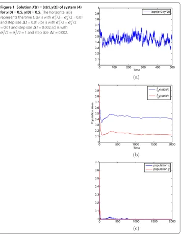
In Figure a,b, we choosea=b= .,a=b= .,c=c= .. In Figure a,b, we chooseσ(t)/ =σ(t)/ = .. By virtue of Theorem , the system will be stochastically permanent. It follows from Theorem  that the system will be persistent in mean. What we mentioned above can be seen from Figure a,b. The diﬀerence between conditions of Figure a,b,c is that the values of σ andσ are diﬀerent. In Figure a,b, we choose

σ_/ =σ_/ = .. In Figure c, we chooseσ_/ =σ_/ = . In view of Theorem , both speciesxandywill go to extinction. Figure c conﬁrms this.

By comparing Figure a,b with Figure c, we can observe that small environmental noise can retain the stochastic system permanent; however, suﬃciently large environmental noise makes the stochastic system extinct.

7 Conclusions

(16)

Figure 1 SolutionX(t) = (x(t),y(t)) of system (4) forx(0) = 0.5,y(0) = 0.5.The horizontal axis represents the timet. (a) is withσ2

1/2 =σ22/2 = 0.01

and step sizet= 0.01; (b) is withσ2 1/2 =σ22/2

= 0.01 and step sizet= 0.002; (c) is with

σ2

1/2 =σ22/2 = 1 and step sizet= 0.002.

desired. However, Theorem  reveals that a large white noise will force the population to become extinct.

Competing interests

The authors declare that they have no competing interests.

Authors’ contributions

The authors carried out the proof of the main part of this article. All authors have read and approved the ﬁnal manuscript.

Author details

1_{Department of Mathematics, Harbin Institute of Technology, Weihai, 264209, P.R. China.}2_{Department of Mathematics,}

Civil Aviation University of China, Tianjin, 300300, P.R. China.3_{School of Mathematics and Statistics, Northeast Normal}

University, Changchun, 130024, P.R. China.

Acknowledgements

(17)

Innovation Foundation in Harbin Institute of Technology (No. HIT.NSRIF.2011094), the Scientiﬁc Research Foundation of Harbin Institute of Technology at Weihai (No. HIT(WH)ZB201103).

Received: 3 February 2012 Accepted: 30 January 2013 Published: 18 February 2013

References

1. Chen, LJ, Chen, LJ, Li, Z: Permanence of a delayed discrete mutualism model with feedback controls. Math. Comput. Model.50, 1083-1089 (2009)

2. Gapalsamy, K: Stability and Oscillations in Delay Equations of Population Dynamics. Kluwer Academic, London (1992) 3. Li, YK, Xu, GT: Positive periodic solutions for an integrodiﬀerential model of mutualism. Appl. Math. Lett.14, 525-530

(2001)

4. Chen, FD, You, MS: Permanence for an integrodiﬀerential model of mutualism. Appl. Math. Comput.186, 30-34 (2007) 5. Mao, XR, Marion, G, Renshaw, E: Environmental Brownian noise suppresses explosions in population dynamics. Stoch.

Process. Appl.97, 95-110 (2002)

6. Jiang, DQ, Shi, NZ, Li, XY: Global stability and stochastic permanence of a non-autonomous logistic equation with random perturbation. J. Math. Anal. Appl.340, 588-597 (2008)

7. Ji, CY, Jiang, DQ, Shi, NZ: Analysis of a predator-prey model with modiﬁed Leslie-Gower and Holling-type II schemes with stochastic perturbation. J. Math. Anal. Appl.359, 482-498 (2009)

8. Li, XY, Mao, XR: Population dynamical behavior of non-autonomous Lotka-Volterra competitive system with random perturbation. Discrete Contin. Dyn. Syst.24, 523-545 (2009)

9. Zhu, C, Yin, G: On hybrid competitive Lotka-Volterra ecosystems. Nonlinear Anal. TMA71, e1370-e1379 (2009) 10. Zhu, C, Yin, G: On competitive Lotka-Volterra model in random environments. J. Math. Anal. Appl.357, 154-170 (2009) 11. Ji, CY, Jiang, DQ, Li, XY: Qualitative analysis of a stochastic ratio-dependent predator-prey system. J. Comput. Appl.

Math.235, 1326-1341 (2011)

12. Chen, LS, Chen, J: Nonlinear Biological Dynamical System. Science Press, Beijing (1993) 13. Mao, XR: Stochastic versions of the Lassalle theorem. J. Diﬀer. Equ.153, 175-195 (1999) 14. Karatzas, I, Shreve, S: Brownian Motion and Stochastic Calculus. Springer, Berlin (1991)

15. Friedman, A: Stochastic Diﬀerential Equations and Applications. Academic Press, New York (1976) 16. Mao, XR: Stochastic Diﬀerential Equations and Applications. Horwood, Chichester (1997)

17. Barbalat, I: Systems d’equations diﬀerential d’oscillations nonlineairies. Rev. Roum. Math. Pures Appl.4, 267-270 (1959) 18. Higham, DJ: An algorithmic introduction to numerical simulation of stochastic diﬀerential equations. SIAM Rev.43,

525-546 (2001)

doi:10.1186/1687-1847-2013-37