Translation, solving scheme, and implementation of a periodic and optimal impulsive state control problem

R E S E A R C H

Open Access

Translation, solving scheme,

and implementation of a periodic

and optimal impulsive state control problem

Ying Song

_{, Yongzhen Pei}

_{, Miaomiao Chen}

_{and Meixia Zhu}

*_{Correspondence:} [email protected] 1_{School of Science, Tianjin} Polytechnic University, Tianjin, China 2_{School of Computer Science and} Software Engineering, Tianjin Polytechnic University, Tianjin, China

Abstract

The periodic solution of the impulsive state feedback controls (ISFC) has been investigated extensively in the last decades. However, if the ecosystem is exploited in a period mode, what strategies are implemented to optimize the cost function at the minimal cost? Firstly, under the hypothesis that the system has a periodic solution, an optimal problem of ISFC is transformed into a parameter optimization problem in an unspecified time with inequality constraints, and together with the constraint of the first arrival threshold. Secondly, the rescaled time and a constraint violation function are introduced to translate the above optimal problem to a parameter selection problem in a specified time with the unconstraint. Thirdly, gradients of the objective function on all parameters are given to compute the optimal value of the cost function. Finally, three examples involving the marine ecosystem, computer virus, and resource administration are illustrated to confirm the validity of our approaches.

Keywords: Impulsive state feedback control (ISFC); Rescaled time transformation; Constraint violation function; Parameter optimization; Numerical simulation

1 Introduction

The topic about impulsive state feedback controls (abbreviated as ISFC) has been investi-gated extensively in the last decades due to its potential applications in culturing microor-ganisms [1–3], pest integrated management [4–6], disease control [7, 8], fish harvesting [9–11], and wildlife management [12, 13]. For example, [1] proposed a bioprocess model with ISFC to acquire an equivalent stable output by the precise feeding. Ref. [4] explored the periodic solution of an entomopathogenic nematode invading the insect model with ISFC. Ref. [7] considered some vaccines into a disease by ISFC, and got the uniqueness of order one periodic solution (OOPS) by geometric method. Ref. [12] formulated a white-headed langur’s ISFC model with sparse effect and continuous delay to study the periodic and artificial releasing. On ISFC models, scholars often pay close attention to the qualita-tive analysis of OOPS. Ref. [11] proposed a phytoplankton–fish model with ISFC and then formulated an optimal control problem (OCP, for short) and strived to find the appropriate harvesting rates to maximize the cost function in an impulsive period. Here, the solvability of the system in one period provides convenience for solving the OCP by Lagrange mul-tiplier. But for the complicated ecosystem whose analytical solution cannot be expressed explicitly, if it is exploited in a period mode, what period and strategies are implemented

to optimize the cost function at the minimal cost? Furthermore, how to translate the OCP of the ISFC to a problem with parameter optimization in one period is interesting. So far, few researchers have paid attention to these tasks which are the focuses of our paper.

The utilizations of optimal control can be found almost in all applied science fields, such as fishery model [14], iatrochemistry [15], switching powers [16], astrovehicle con-trols [17], undersea vehicles [18], eco-epidemiology [19], and virus therapies [20]. The Pontryagin principle and the Hamilton equation are the main theoretical tools to solve continuous system control [21]. However, the hybrid optimization problems involving the pulse threshold and system parameters are still sufficiently challenging and worth explor-ing. The control parameter technique offers the feasibility for solving this problem [21]. Teo et al. described the detailed and basic theory of the control parameter method in [22]. Until now, many important results have been achieved in recent years. We will apply these theories together with the constraint transcription technique [23] to resolve the above is-sues.

The other components of this paper are as follows. In Section 2, an optimal problem of state impulse feedback control is transformed into a parameter optimization problem in an unspecified time with inequality constraint, and together with the constraint of the first arrival threshold. In Section 3 we derive the required gradient formulas and present an algorithm for solving the approximate OCP. In Section 4, we give three examples and numerical simulations. Finally, a conclusion is provided in Section 5.

2 Problem statement and translation Consider the ISFC system:

(H1) Assume thatfi,φ, andIare continuously differentiable.

(H2) Denote the Euclidean norm by · . Suppose that there exists a constraintk> 0

meeting|fi(yˆ)| ≤k(1 +ˆy)for allyˆ.

(H3) Assume that for fixedyˆ₀, (2.1) and (2.2) have a unique OOPSA→Bpossessing

periodT, whereAandBare the terminal and initial points of OOPS, respectively. When the impulsive effect take places, the pointAis mapped toB, namely

Aˆy1(T) +I1

ˆ

y(T),β, . . . ,yˆn(T) +In

ˆ

y(T),β→B(yˆ10, . . . ,yˆn0).

Next, our aim is to formulate an optimal problem on one period under hypothesis (H3), namely (2.1) and (2.2) possess an OOPSA→B. Then system (2.1) is modified into

dyˆ

dt =f(ˆy,δ), t∈(0,T). (2.3)

By (H3) it is obtained that

ˆ

yi0=yˆi(T) +Ii

ˆ

y(T),β, i= 1, . . . ,n. (2.4)

In order to guarantee thatTis the first positive time at which the solutionyˆ(t) of (2.1) intersects with the surfaceφ(ˆy(t),δ) = 0,yˆ(t) should be defined as follows:

(H4) yˆ(t)∈, where

=yˆ(t)|φyˆ(t),δ= 0fort∈(0,T)andφyˆ(T),δ= 0. (2.5)

Remark IfT is not the first positive time at which the solutionyˆof (2.1) intersects with the surfaceφ(ˆy(t),δ) = 0, then there exists 0 <T˘<Tsuch thatφ(yˆ(T˘),δ) = 0. This appears in contradiction to the definitions of (2.5).

Obviously, (2.5) is equivalent to

=yˆ(t)|φyˆ(t),δ>φyˆ(T),δorφyˆ(t),δ<φyˆ(T),δfort∈(0,T). (2.6)

Together with (2.4), the solution which firstly arrives at the surfaceφ(ˆy(T),δ) = 0 at time

T from the initial point (0,yˆ₀) (that is, the solution in (2.5) or (2.6)) is renewed by =yˆ(t),yˆ₀< 0 and∗yˆ(t),yˆ(T)< 0,t∈(0,T). (2.7) Define admissible setsand , which have respectivelypandqdimensions, such that

δ∈,β∈ . Then, for each (δ,β)∈× , the boundary condition of the mixed type (2.4) is equivalently expressed as

yˆ₀,yˆ(T|δ,β)= 0, (2.8)

where= (1, . . . ,n)T is ann-dimensional vector function. Clearly, the terminal time

(H5) Assume thati,, and∗are continuously differentiable. Next, we give the cost (objective) function:

J0= 0

ˆ

y(δ)(T),β+

T

0

L0

ˆ

y(δ)(t)dt, (2.9)

where 0∈Rn→Rdefines the terminal cost andL0 defines the running cost.

Equa-tion (2.9) also can be called the objective funcEqua-tion [21]. Assume that 0andL0satisfy the following conditions.

(H6) 0is continuously differentiable.

(H7) FunctionsL0are continuously differentiable concerning the componentyˆfor each

t∈[0,Tˆ]. Additionally, there is a constraintl> 0such that|L0(yˆ)| ≤l(1 +ˆy)for

allyˆ.

Now, an OCP is formulated officially as follows:

(P0) Subject to (2.3), seek a parameter vector(δ,β)∈× satisfying that the objective

function (2.9) is minimized over× . HereTis a period meeting conditions (2.7) and (2.8).

In particular, if the solutionyˆ(t) (t∈(0,T)) of (2.1) and (2.2) is monotonic, then (2.7) is rewritten as

ˆ

yi0<yˆi(t) <yˆi(T) or yˆi(T) <ˆyi(t) <yˆi0, i= 1, . . . ,n,t∈(0,T), (2.10)

which ensures thatT is the first positive time of the solutionyˆ(t) arriving at the surface φ(ˆy(t),δ) = 0. Correspondingly, combined with (2.4), (2.10) is equivalently adapted by

i

ˆ

yi(t),ˆyi0

< 0, i= 1, . . . ,n, _j∗yˆj(t),yˆj(T)< 0, j= 1, . . . ,n. (2.11)

3 Solving scheme

The variability of jump time increases the difficulty in solving the problem (P0). To

cir-cumvent this difficulty, we choose the time-scaling transformation technology called the control parameter enhancing transform ( CPET, for short). Ref. [24] firstly preferred CPET to ascertain optimal switching instants for time-optimal controls. Afterwards, we employ CPET to project the variable jump times to fixed points by an updated time scale, thus an updated optimal issue with the fixed jump times is yielded. For applying this method, we introduce the rescaled time [24, 25]

s=t/T. (3.1)

Obviously, system (2.3) is rewritten as

dy

ds =h(y,δ,T), (3.2)

wheres∈(0, 1). Here we refer toT as an organic parameter which is a decision variable. In addition,

y(s) =yˆ(Ts),

Then (2.7) and (2.8) can be respectively expressed as

y(s),y₀< 0, ∗y(s),y(1)< 0, s∈(0, 1), (3.3)

and

y₀,y(1),β= 0. (3.4)

And the cost function (2.9) is equivalent to

J1= 0

y(1),β+ 1

0

L0

y(s),δ,Tds, (3.5)

with

0

y(1),β= 0

ˆ

y(δ)(T),β, L0

y(s),δ,T=TL0(ˆy(δ)(t).

Thus, we can change the problem (P0) into the following problem:

(P1) Given system (3.2), find a combined parameter vector(δ,β,T)∈× ×(0,Tˆ)to

minimize the objective functional (3.5) and meanwhile satisfy (3.3) and (3.4).

By Theorems in [25] and [26], the next result is valid.

Lemma 3.1 The OCP(P0)⇔the problem(P1).

Next, we recommend an exact penalty method to overcome the remaining difficulty that the constraints (3.3) define a disjoint feasible region. Such constraints are referred to as functional inequality or path constraints. The essential dilemma about these constraints lies in the innumerable restriction on the state variables in the time scale [21].

Constraint (3.3) is a non-standard “open” state constraint. So we can approximate it as follows:

y(s),y₀≤ ¯ε, ∗y(s),y(1)≤ ¯ε, s∈[δ, 1 –δ], (3.6)

whereε¯> 0 andδ∈(0,1₂) are adjustable parameters. Then, we define a constraint violation function as

(δ,β,T) =y₀,y(1),β2

+T

1 0

maxε¯,y(s),y₀2+maxε¯,∗y(s),y(1)2ds. (3.7)

Note that(δ,β,T) = 0 if and only if (3.3) and (3.4) hold. By the strategy presented in [27–30], one sets up an exact penalty function

J2(δ,β,T,ε) =

⎧ ⎪ ⎨ ⎪ ⎩

J1(δ,β,T), ifε= 0 and(δ,β,T) = 0,

J1(δ,β,T) +ε–α(δ,β,T) +σ εγ, ifε> 0,

whereσ > 0 is a positive penalty parameter.α> 0 andγ > 0 are constants meeting 1≤ γ ≤α. The new decision variableεsatisfies

0≤ε≤ε1, (3.8)

whereε1is a small positive number. This method was first mentioned in [31].

Now we give the unconstrained control problem:

(P2) Optimize a combined parameter vector(δ,β,T)∈× ×(0,Tˆ)and the new

decision variableε∈[0,ε1]to minimize the transformed equivalent cost function

J2(δ,β,T,ε)subject to the dynamics given by (3.1) and (3.2) in the interval(0, 1).

According to the main convergence result of [29], whenε¯andδapproach zero, the cost ofJ2approaches the optimal costJ1of problem (P2).

Theorem 3.1 Letι> 0be an arbitrary fixed number.For any enough smallδ> 0,we can find a corresponding positive pointε¯1(δ) > 0such that

|J2–J1|<ι, ε¯∈(0,ε¯1].

The above approximate problem is a nonlinear optimization one. For minimizing the objective function which subjects to a group of constraints, the narrow decision variables are selected. And for the decision vector, the cost and objective functions are implicit in problem (P2). Then we can develop their gradients to produce search directions which

guide profitability for the search space [21]. For implementing these algorithms, it is es-sential to compute the partial derivatives of the final cost function. A method for comput-ing gradients is the so-called costate method. From Theorem 4.1 in [32] and Section 5.2 in [33], we define the corresponding Hamiltonian function

Hs,y(s),y(1),λ(s),δ,T,ε=L0

y(s),δ,β,T+λTh(y,δ,T)

+ε–νTmaxε¯,y(s),y₀2

+maxε¯,∗y(s),y(1)2, (3.9)

whereλT(s) = (λ1(s), . . . ,λn(s)) andλi(s) is the corresponding costate fori= 1, 2, . . . ,n.

Fur-thermore,λ(s) is determined by the following differential equations:

dλ

ds = –

∂H(s,y(s),y(1),λ(s),δ,T,ε) ∂y

T

, (3.10)

λT(1) = ∂ 0 ∂y(1)+ 2ε

–α_y

0,y(1),β

2 ∂

∂y(1)+ 1

0

∂H

∂y(1)ds. (3.11)

Theorem 3.2 The gradients of J2concerning T,δ,βas well asεare awarded by

∂J2

∂T =

1 0

∂H

∂T ds, (3.12)

∂J2

∂δ = 1

0

∂H

∂J2

Note that, instead of an initial condition, the costate systems (3.10) and (3.11) involve a terminal value. So, we must integrate them froms= 1 tos= 0. Furthermore, in view of equations (3.12)–(3.15), we address the algorithm about calculatingJ2and its gradients as

follows.

∂β according to equations (3.12), (3.13),

and (3.14).

In the above, the methodology proposed involves transforming the periodic optimal control problem into a standard optimal control problem, after which standard computa-tional techniques can be applied. Similarly, the case of the first positive timeTassured by (2.11) can be derived.

4 Application

In this section, three examples are given to implement the above theories and approaches; and furthermore, to verify the validity of our algorithm.

Example 4.1 (Phytoplankton–fish system) Consider the following impulsive system

[11]:

Herep0andz0present respectively the initial levels of phytoplankton and fish. From

The-orems 3.1 and 4.3 in [11], it is obtained that for fixed (p0,z0) system (4.1) has an OOPS

A→BfromA((1 –e1)p1, (1 –e2)H) toB(e1,H). Then Zhao et al. [11] formulated an OCP

and strived to seek the appropriate harvesting ratese∗₁ande∗₂to maximize the cost func-tionJ(e1,e2) =C1e1p1+C2e2Hin an impulsive period.C1andC2describe the prices per

unit biomass of the phytoplankton and fish, respectively.

In our paper, based on the periodic solution theory in [11], we know that the re-sources are exploited in a period mode. Then, what strategies are implemented to op-timize the cost function at the minimal cost? For this, we take the harvesting ratese1,

e2 and the harvest period T as control parameters to achieve the maximal revenue,

Combined with the periodicity of harvesting, the solution (p(t),z(t)) of system (4.1) on (0,T] meets the following conditions:

_dp

dt = (r–az)p, dz

dt= (bp–u– dp

γ+p)z,

t∈(0,T), (4.2)

p(T) = p0 1 –e1

, z(T) =H= z0 1 –e2

. (4.3)

Furthermore, together with the monotonicity ofz(t), it is obtained

z(0) <z(t) <z(T), (4.4)

whereTalso is the first positive time such that (4.3) and (4.4) hold.

After the rescaled time transformation, (4.2), (4.3), and (4.4) can be rewritten as fol-lows:

dp

ds =T(r–az)p . =f1,

dz

ds=T(bp–u– dp

γ+p)z . =f2,

fors∈(0, 1), (4.5)

p(1) = p0 1 –e1

, z(1) =H= z0 1 –e2

, (4.6)

z(0) <z(s) <z(1). (4.7)

Our cost function can be expressed as follows: subject to (4.5)–(4.7),

min e1,e2,T

J2(e1,e2)

= min

e1,e2,T

–C1e1p(1) –C2e2z(1)

.

For system (4.5)–(4.7), define the violent function by

(e1,e2,T) =

(1 –e1)p(1) –p0

2

+(1 –e2)z(1) –z0

2

+T

1 0

maxε¯,z(0) –z(s)2+maxε¯,z(s) –z(1)2. (4.8)

Noting that(e1,e2,T) = 0 if and only if constraints (4.6) and (4.7) are satisfied, then our

cost functionJ2(e1,e2) turns into

J3(e1,e2) = –C1e1p(1) –C2e2z(1) +ε–v(e1,e2,T) +σ εw. (4.9)

After that, the corresponding Hamiltonian function is

Hs,p(s),z(s),λ1(s),λ2(s),T,ε

=λ1f1+λ2f2

+Tmaxε¯,z(0) –z(s)2

whereλ1(s) andλ2(s) are determined by the auxiliary system:

The parameters are chosen as

r= 1.144, a= 0.2, b= 0.2, d= 0.5, γ = 2, u= 0.5,

v= 2, w=1.55, ε¯= –1e–8, σ= 100, C1= 3, C2= 2,

(4.16)

with the initial valuesp0= 7,z0= 1. For the initial guessesT0= 3,e10= 0.7,e20= 0.9, and

ε0= 0.1, we obtain that the cost functionJ0= 1634.15 and the thresholdh0=S(T0) = 13.64.

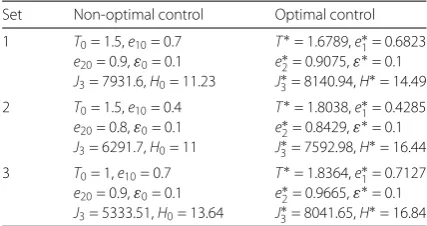
Furthermore, by the costate equations and transversality conditions in (4.5) as well as the gradients (4.12)–(4.15), starting with the above initial values, we recover the optimal con-trol scheme showed in Table 1. Apparently, the harvest periodTis extended, harvesting ratese1ande2are enlarged, and our final gains are also increased after our optimal

con-trol. Additionally, we adapt this set of data to plot the phase diagram of food and species according to the optimal and initial controls, respectively (see Figure 1). The red circle

Table 1 Results of simulation 1

Figure 1Phase portrait of (4.1) with optimal and non-optimal controls on one period (0,T]

represents the trajectories of populations on the basis of the optimal scheme, whereas the blue solid line represents the trajectory under the initial scheme. From Figure 1, we also notice that the threshold of plankton also increases, which is consistent with the results in Table 1. Summarily, our optimal tactics not only delay the harvest but also magnify the harvesting threshold and benefit, which are desirable for human exploitation.

Example4.2 (Computer virus propagation under media coverage) In this section, a new

computer virus model with state impulsive control [8, 34, 35] is utilized to exemplify our algorithm and approach:

⎧ ⎪ ⎪ ⎪ ⎪ ⎨ ⎪ ⎪ ⎪ ⎪ ⎩

ds

dt=g–ds+ni– (b1–b2 i m+i)si, di

dt= (b1–b2 i

m+i)si–ni–di,

i<H,

s= –e1s,

i= –e2i,

i=H,

(4.17)

wherendenotes the recovery rate from an infected computer to a susceptible one due to the application of antivirus software.b1denotes the contact rate at which the susceptible

computer gets infected before media alert,b2is the maximum reduction of contact rate

through media coverage, andm> 0 represents the effect of media coverage.

For (4.17), the existence together with stability of OPS have been showed in [8]. Then, in the following, we analogously formulate an optimal state pulse control problem of system (4.17) on a period (0,T]:

_ds

dt=g–ds+ni– (b1–b2 i m+i)si, di

dt= (b1–b2 i

m+i)si–ni–di,

t∈(0,T), (4.18)

wheres(t) andi(t) satisfy the inequality constraint

i(t) <i(T), (4.19)

and equality constraints

s(T) = s0 1 –e1

, i(T) = i0 1 –e2

. (4.20)

Next we build the cost function. Namely, subject to (4.18)–(4.20), find the appropriate

wherep1andp2denote the cost of susceptible and infected computers andωis the weight

factor.

Utilizing the time scale transformation and the violent violation function, the optimal solution of the above control problem is determined by the following system:

Next, we give the simulation of Example 4.2. In system (4.17), a set of parameter values is chosen as

g= 0.3, d= 0.18, n= 0.18, b1= 0.65, m= 3, v= 2,

w= 1.55, ε¯= –1e–8, σ= 100, p1= 1, p2= 2, ω= 0.5

Table 2 Results of simulation 2

Set Non-optimal control Optimal control

1 T= 8,b2= 0.6,ε0= 0.1 T∗= 6.5499,b∗2= 0.6214,ε∗= 4.521e–5

e1= 0.8,e2= 0.9 e∗1= 0.1613,e∗2= 0.4572

J1= 69.4267,H= 0.7347 J∗= 1.36176,H∗= 0.6632

2 T= 7,b2= 0.55,ε0= 0.1 T∗= 6.1392,b∗2= 0.6345,ε∗= 1.61e–6

e1= 0.7,e2= 0.6 e∗1= 0.1703,e∗2= 0.4371

J1= 53.4043,H= 0.7005 J∗= 0.7111,H∗= 0.6396

3 T= 6,b2= 0.5,ε0= 0.1 T∗= 5.9094,b∗2= 0.5386,ε∗= 0.441e–7

e1= 0.2,e2= 0.4 e∗1= 0.1553,e∗2= 0.4422

J1= 32.5521,H= 0.6578 J∗= 0.6984,H∗= 0.6454

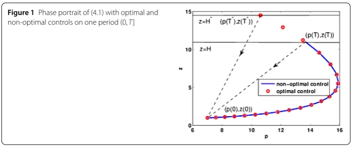
Figure 2Phase portrait of system (4.17) with optimal and non-optimal controls on one period (0,T]

with the initial values0= 0.68 andi0= 0.36. In Table 2, we give three sets of parameter

ini-tial values to compute the minimal cost functionJ∗and to find the appropriate parameters. From Table 2, we find that after optimal control the contact rateb2through media

cover-age is increased, while the periodTis shortened, the number of the infected computers is maintained at a low levelH∗and the cost is reduced. That is, increasing the influence of media and taking regular anti-virus measures for a computer will reduce the cost of pre-vention and control of computer viruses. Furthermore, we display the dynamic behavior of susceptible and infected computers and the optimal thresholdH∗in Figure 2 with the first set of Table 2. All of the red cycles illustrate the behaviors of susceptible and infected computers when optimal control action is taken, while all of the blue solid lines present the habit of susceptible and infected computers when non-optimal control is taken.

Example4.3 (Species-food system) After our little sojourn in the simple examples, it is time to return to a complex example. Consider the following system in [36]:

⎧ ⎪ ⎪ ⎪ ⎪ ⎪ ⎪ ⎨ ⎪ ⎪ ⎪ ⎪ ⎪ ⎪ ⎩

dx

dt = –γxy, dy

dt = –y(–δx),

ifx=x1,

x(τk) =λ,

y(τk) =

0, ifkis not divisible byn, –αy(τk), ifkis divisible byn,

⎫ ⎪ ⎬ ⎪

⎭ ifx=x1,

(4.32)

the moments of the impulse effectτkwhose ordinal numberkis a multiple ofn. We also assumed thatλ> 0 and 0 <α< 1.

Based on the research of the period solution in [36], we propose our optimal problem on the condition that (4.32) admits a periodic solution with periodT. According to the theory in Section 2, we can rewrite system (4.32) on one period (0,T) as follows:

⎧ ⎪ ⎪ ⎪ ⎪ ⎪ ⎪ ⎪ ⎪ ⎪ ⎨ ⎪ ⎪ ⎪ ⎪ ⎪ ⎪ ⎪ ⎪ ⎪ ⎩

dx

dt = –γxy, dy

dt = –y(–δx),

ift=τk,k= 1, 2, . . . ,n,k∈Z+,τk∈(0,T], x=λ,

y= 0,

ift=τk,k= 1, 2, . . . ,n– 1,

x=λ, y= –αy,

ift=τn,

(4.33)

wherenis a positive integer representing the number of releasing food. Furthermore, the populations of the food and the species meet the following restraints on (0,T]:

x(τ_k+_–1) >x(t) >x(τk), k= 1, 2, . . . ,n,

y(τ_k+_–1) <y(t), k= 1, 2, . . . ,n, (4.34)

x(τk) +λ=x0, k= 1, 2, . . . ,n, y(T) =y(τn) =

y0

1 –α, (4.35)

whereτnis also the first positive time such that (4.35) holds. Thus, our OCP can be written as follows.

Problem (P0): In order to minimize the cost of the total releasing food and maximize the

quality of species at the terminal time, we would like to findλandαto minimize the cost function

J₀n=p1nλ–p2αy(T),

wherep1andp2denote the market prices of the food and species.

First, the time scaling transformation is utilized to project the impulsive moments

t= 0,τ1,τ2, . . . ,τnintos= 0, 1, 2, . . . ,nin a new time horizon. Define the required trans-formation:

dt(s)

ds =v(s) (4.36)

witht(0) = 0.v(s) is the time scaling control function and is discontinuous ats= 1, 2, . . . ,n. That is,

v(s) = n

k=1

¯

τkχ(k–1,k)(s), (4.37)

whereτ¯k=τk–τk–1is the duration which satisfies the following condition:

n

k=1

¯

Define the indicator function ofIby

χI(s) =

1, ifs∈I,

0, otherwise. (4.39)

By time scaling transformation, systems (4.33)–(4.35) turn into ⎧

Thus we can change problem (P0) into the next problem.

Problem (P1): Minimize the transformed cost function

J₁n=p1nλ–p2αy(n)

by selectingλandα.

This optimal problem has multi-jump times, which differs from the first two examples and is difficult to solve. For this, time translation transformation will be introduced [37]. Define

Further, the cost functionJ₁nis rewritten as follows:

In view of (3.7), we define a constraint violation function

minimize the transformed equivalent cost function

J₃n=p1nλ–p2αyn(1) +ε–a+σ εb

subject to (4.44)–(4.46) as well as the restraints 0 <α< 1 andλ> 0.

Next, according to Theorem 4.1 in [38] and [32], we define the corresponding Hamilto-nian function

Hi=ε–aτ¯i

maxxi(s) –xi(0),ε¯2+maxxi(1) –xi(s),ε¯2

+maxyi(0) –yi(s),ε¯2+li₁f₁i+li₂f₂i fori= 1, 2, . . . ,n, (4.48)

wherel₁i andl₂i are determined by the auxiliary system: ⎧

Now we give the derivatives ofJn

Table 3 Results of simulation forn= 5

Set Non-optimal control Optimal control

1 τ1= 3.23,τ2= 1.98,τ3= 1.44 τ1∗= 2.99,τ2∗= 1.77,τ3∗= 1.26 τ4= 1.13,τ5= 0.94 τ4∗= 0.98,τ5∗= 0.81

λ= 4.51,α= 0.8773,ε0= 0.1 λ∗= 4.4,α∗= 0.89,ε∗= 6.581e–5

J5

3= 18.2467,x1= 0.49 J53∗= 14.1559,x1∗= 0.6 2 τ1= 2.35,τ2= 1.27,τ3= 0.88 τ1∗= 2.34,τ2∗= 1.26,τ3∗= 0.876

τ4= 0.67,τ5= 0.54 τ4∗= 0.67,τ5∗= 0.54

λ= 4,α= 0.9028,ε0= 0.1 λ∗= 3.99,α∗= 0.9029,ε∗= 71e–5

J5

3= 13.5705,x1= 1 J53∗= 10.6311,x1∗= 4 3 τ1= 4.77,τ2= 3.82,τ3= 3.2 τ1∗= 4.74,τ2∗= 3.80,τ3∗= 3.17

τ4= 2.76,τ5= 2.44 τ4∗= 2.73,τ5∗= 2.40

λ= 4.8,α= 0.7724,ε0= 0.1 λ∗= 4.79,α∗= 0.7274,ε∗= 21e–4

J5

3= 24.2191,x1= 0.2 J53∗= 21.30982,x∗1= 0.21

Next, the simulation of Example 4.3 is given. Choose (x0,y0) = (5, 0.5). The parameter

values are taken as

γ = 0.6, = 0.4, δ= 0.3, a= 2, b= 1.55,

¯

ε= –1e–8, σ= 100, p1= 1, p2= 2, λ= 4.5, α= 0.8773.

(4.54)

The optimal problem is solved by using a Matlab program and the above computational approach.

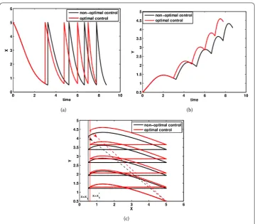
Taken= 5 which implies that the food is released five times and the species is harvested one time on one period (0,T]. Then the simulation results of system (4.32) are listed in Table 3 for various parameters. Here, the optimal time intervalsτ₁∗,τ₂∗,τ₃∗,τ₄∗, andτ₅∗are shortened, which consequently gives rise to the shortness of periodT. Also the optimal increment of foodλ∗is decreased slightly, meanwhile the optimal harvesting rateα∗keeps invariable and the cost valueJ35∗is reduced. Also Figure 3(c) visualizes the optimal control

strategy that less food is released at every impulsive time and more amount of species is acquired at the terminal time. We plot the time evolutions of food and species according to the optimal and non-optimal control laws with the first set of Table 3 (see Figures 3(a) and (b)). The black line means the dynamic behavior of non-optimal control and the red line means the dynamic behavior of optimal control. Obviously, the optimal tactics partly promotes the level of the species, which is desirable from the protection population.

Next, we consider the case ofn= 1, which implies that the food is released and the species is harvested one time on one period (0,T], respectively. The results obtained are shown in Table 4 for three sets of parameters. For given initial intervalT, initial recruit-ment rateα, our goal is to compute the minimal cost functionJ₃1∗with time intervalT∗, release amountλ∗and the capture rateα∗. We explore that control policy not only drops the level of the cost function, but also boosts the numbers of species at the terminal time. Meanwhile, the time interval is shortened too. Graphical output in Figure 4(c) directly displays our optimal control strategy expressed by (4.32) withn= 1. All of the black lines illustrate the behaviors of non-optimal control while all of the red lines mean the dynamic behavior of optimal control. When optimal control strategy is implemented, the trajecto-ries of food and species are drawn in Figures 4(a) and (b). It shows that the level of species is higher in an optimal mode than in a non-optimal one at the terminal time.

(a) (b)

(c)

Figure 3Comparisons of system (4.32) with optimal and non-optimal controls on one period (0,T] with

n= 5. (a) and (b) are the time series of food and species, (c) is the phase portrait

Table 4 Results of simulation forn= 1

Set Non-optimal control Optimal control 1 T= 3.23,λ= 4.51 T∗= 2.93,λ∗= 4.37

α= 0.5881,ε= 0.1 α∗= 0.62,ε∗= 1.57e–4

J1

3= 3.65,x1= 0.49 J31∗= 2.77,x∗1= 0.63 2 T= 2.35,λ= 4 T∗= 2.31,λ∗= 3.96 α= 0.6501,ε= 0.1 α∗= 0.65,ε∗= 9e–5

J13= 2.71,x1= 1 J31∗= 2.01,x∗1= 1.04 3 T= 4.77,λ= 4.8 T∗= 4.42,λ∗= 4.76

α= 0.2952,ε= 0.1 α∗= 0.41,ε∗= 2.64e–4

J1

3= 4.94,x1= 0.2 J31∗= 4.05,x∗1= 0.24

Compared withJ5∗

3 , which represents that the moden= 5 is executed one time, it

indi-cates that the cost function 5J₃1∗is slightly less thanJ₃5∗. This result implies that the control mode of frequent releasing food and frequent harvest species is superior to that of fre-quent releasing food and infrefre-quent harvest species.

5 Discussions

(a) (b)

(c)

Figure 4Comparisons of system (4.32) with optimal and non-optimal controls whenn= 1. (a) and (b) are the time series of food and species, (c) is the phase portrait

However, if the system is exploited in a period mode, what strategies are implemented to achieve the objective of optimal management? So far, few researchers keep a watchful eye on this task which has been our focus in the above sections. In summary, our approaches are concluded by the following three procedures. (1) Under the hypothesis that the ISFC system has a periodic solution, an optimal problem of ISFC is transformed into a parame-ter optimization problem in an unspecified time with inequality constraint, and together with the constraint of the first arrival threshold. (2) The rescaled time and a constraint violation function are introduced to translate the above optimal problem to a parameter selection problem in a specified time with the unconstraint. (3) The gradients of the ob-jective function on all of parameters are given to compute the optimal value of the cost function. Finally, three examples involving the marine ecosystem, computer virus control, and resource administration are illustrated to confirm the validity of our approaches. In these examples, the parameters of the impulse and system on continuous systems and a hybrid system are optimized respectively.

Acknowledgements

The authors thank the referees for their careful reading of the original manuscript and many valuable comments and suggestions that greatly improved the presentation of this paper.

Funding

This work was supported by the National Natural Science Foundation of China (11471243, 11501409). Competing interests

The authors declare that they have no competing interests. Authors’ contributions

All authors contributed equally to the manuscript and read and approved the final draft.

Publisher’s Note

Springer Nature remains neutral with regard to jurisdictional claims in published maps and institutional affiliations.

Received: 1 November 2017 Accepted: 6 February 2018

References

1. Tian, Y., Sun, K., Chen, L., Kasperski, A.: Studies on the dynamics of a continuous bioprocess with impulsive state feedback control. Chem. Eng. J.157(2), 558–567 (2010)

2. Li, Z., Chen, L., Liu, Z.: Periodic solution of a chemostat model with variable yield and impulsive state feedback control. Appl. Math. Model.36(3), 1255–1266 (2012)

3. Zhao, Z., Yang, L., Chen, L.: Impulsive state feedback control of the microorganism culture in a turbidostat. J. Math. Chem.47(4), 1224–1239 (2010)

4. Sun, K., Tian, Y., Chen, L., Kasperski, A.: Nonlinear modelling of a synchronized chemostat with impulsive state feedback control. Math. Comput. Model.52(1–2), 227–240 (2010)

5. Wei, C., Chen, L.: Homoclinic bifurcation of prey–predator model with impulsive state feedback control. Appl. Math. Comput.237(7), 282–292 (2014)

6. Tang, S., Tang, B., Wang, A., Xiao, Y.: Holling II predator–prey impulsive semi-dynamic model with complex Poincaré map. Nonlinear Dyn.81(3), 1575–1596 (2015)

7. Guo, H., Chen, L., Song, X.: Dynamical properties of a kind of sir model with constant vaccination rate and impulsive state feedback control. Int. J. Biomath.10, Article ID 1750093 (2017)

8. Zhang, M., Song, G., Chen, L.: A state feedback impulse model for computer worm control. Nonlinear Dyn.85(3), 1561–1569 (2016)

9. Wei, C., Chen, L.: Heteroclinic bifurcations of a prey–predator fishery model with impulsive harvesting. Int. J. Biomath.

6, Article ID 1350031 (2013)

10. Guo, H., Chen, L., Song, X.: Qualitative analysis of impulsive state feedback control to an algae–fish system with bistable property. Appl. Math. Comput.271, 905–922 (2015)

11. Zhao, Z., Pang, L., Song, X.: Optimal control of phytoplankton–fish model with the impulsive feedback control. Nonlinear Dyn.88, 2003–2011 (2017)

12. Chen, S., Xu, W., Chen, L., Huang, Z.: A white-headed langurs impulsive state feedback control model with sparse effect and continuous delay. Commun. Nonlinear Sci. Numer. Simul.50, 88–102 (2017)

13. Guo, H., Song, X., Chen, L.: Qualitative analysis of a Korean pine forest model with impulsive thinning measure. Appl. Math. Comput.234(234), 203–213 (2014)

14. Run, Y.U., Leung, P.: Optimal partial harvesting schedule for aquaculture operations. Mar. Resour. Econ.21(3), 301–315 (2006)

15. Martin, R.B.: Optimal control drug scheduling of cancer chemotherapy. Automatica28(6), 1113–1123 (1992) 16. Loxton, R.C., Teo, K.L., Rehbock, V., Ling, W.K.: Optimal switching instants for a switched-capacitor DC/DC power

converter. Automatica45(4), 973–980 (2009)

17. Açıkme¸se, B. Blackmore, L.: Lossless convexification of a class of optimal control problems with non-convex control constraints. Automatica47, 341–347 (2011)

18. Chyba, M., Haberkorn, T., Smith, R.N., Choi, S.K.: Design and implementation of time efficient trajectories for autonomous underwater vehicles. Ocean Eng.35(1), 63–76 (2008)

19. Liang, X., Pei, Y., Zhu, M., Lv, Y.: Multiple kinds of optimal impulse control strategies on plant–pest–predator model with eco-epidemiology. Appl. Math. Comput.287–288, 1–11 (2016)

20. Pei, Y., Li, C., Liang, X.: Optimal therapies of a virus replication model with pharmacological delays based on reverse transcriptase inhibitors and protease inhibitors. J. Phys. A, Math. Theor.50, Article ID 455601 (2017).

https://doi.org/10.1088/1751-8121/aa8a92

21. Lin, Q., Loxton, R., Teo, K.L.: The control parameterization method for nonlinear optimal control: a survey. J. Ind. Manag. Optim.10(1), 275–309 (2017)

22. Teo, K.L., Goh, C.J., Wong, K.H.: A Unified Computational Approach to Optimal Control Problems. Longman, Harlow (1991)

23. Caccetta, L., Loosen, I., Rehbock, V.: Computational aspects of the optimal transit path problem. J. Ind. Manag. Optim.

4(1), 95–105 (2017)

24. Lee, H.W.J., Teo, K.L., Rehbock, V., Jennings, L.S.: Control parametrization enhancing technique for time-optimal control problems. Dyn. Syst. Appl.6(2), 243–262 (1997)

25. Teo, K.L., Goh, C.J., Lim, C.C.: A computational method for a class of dynamical optimization problems in which the terminal time is conditionally free. IMA J. Math. Control Inf.6(1), 81–95 (1989)

27. Jiang, C., Lin, Q., Yu, C., Teo, K.L., Duan, G.R.: An exact penalty method for free terminal time optimal control problem with continuous inequality constraints. J. Optim. Theory Appl.154(1), 30–53 (2012)

28. Yu, C., Teo, K.L., Bai, Y.: An exact penalty function method for nonlinear mixed discrete programming problems. Optim. Lett.7(1), 23–38 (2013)

29. Lin, Q., Loxton, R., Teo, K.L., Wu, Y.H., Yu, C.: A new exact penalty method for semi-infinite programming problems. J. Comput. Appl. Math.261(4), 271–286 (2014)

30. Yu, C., Teo, K.L., Zhang, L., Bai, Y.: A new exact penalty function method for continuous inequality constrained optimization problems. J. Ind. Manag. Optim.6(4), 559–576 (2010)

31. Teo, K., Goh, C.: A simple computational procedure for optimization problems with functional inequality constraints. IEEE Trans. Autom. Control32(10), 940–941 (2003)

32. Liu, Y., Teo, K.L., Jennings, L.S., Wang, S.: On a class of optimal control problems with state jumps. J. Optim. Theory Appl.98(1), 65–82 (1998)

33. Rui, L.: Optimal Control Theory and Application of Pulse Switching System. University of Electronic Science and Technology Press, Chengdu (2010)

34. Tchuenche, J.M., Dube, N., Bhunu, C.P., Smith, R.J., Bauch, C.T.: The impact of media coverage on the transmission dynamics of human influenza. BMC Public Health11(Suppl. 1), S5 (2011)

35. Li, Y., Cui, J.: The effect of constant and pulse vaccination on sis epidemic models incorporating media coverage. Commun. Nonlinear Sci. Numer. Simul.14(5), 2353–2365 (2009)

36. Li, X., Bohner, M., Wang, C.K.: Impulsive Differential Equations. Pergamon, Elmsford (2015)

37. Wu, C.Z., Teo, K.L.: Global impulsive optimal control computation. J. Ind. Manag. Optim.2(2), 435–450 (2017) 38. Teo, K.L.: Control parametrization enhancing transform to optimal control problems. Nonlinear Anal., Theory