Dynamical behavior of a generalized eco epidemiological system with prey refuge

(1)

R E S E A R C H

Open Access

Dynamical behavior of a generalized

eco-epidemiological system with prey refuge

Shufan Wang

1

_{, Zhihui Ma}

2*

_{and Wenting Wang}

1

*_{Correspondence:}

[email protected]

2_{School of Mathematics and}

Statistics, Lanzhou University, Lanzhou, China

Full list of author information is available at the end of the article

Abstract

A generalized eco-epidemiological system with prey refuge is proposed in this paper. The saturation incidence kinetics and a generalized functional response are used to describe the contact process and the predation process, respectively. Based on mathematical issue, the local and global stability properties, Hopf bifurcation, and permanence of the dynamical system are investigated. Based on the ecological aspects, the impact of prey refuge on the dynamical consequences of the

eco-epidemiological system and the mechanism of prey refuge are discussed. The results reveal that the stabilizing and destabilizing eﬀects occur under some certain conditions. Based on epidemiological issue, the controlling strategies of the infectious disease are proposed. The results show that the prey refuge can control the spread of disease by the relative level of prey refuge. This study has resolved some basic and interesting issues for an eco-epidemiological system with a generalized response function and the eﬀect of prey refuge.

Keywords: Eco-epidemiological system; Generalized function response; Prey refuge; Dynamical behavior; Stabilizing/Destabilizing eﬀect; Method of disease control

1 Introduction

Eco-epidemiological systems, which are applied to describe predator and prey interactions with diseases in one population or both populations, have become important tools in ana-lyzing the spread and control of infectious diseases, and hence have received much atten-tion since the Kermac–Mckendric SIR model was proposed [1–10]. In eco-epidemiology, researchers study an ecological system with disease either in prey or in predator or in both populations [10–16]. Anderson and May [1] proposed an animal (predator) and plant (prey) model with infectious diseases and investigated the invasion, persistence, and spread of diseases. Chattopadhyay et al. investigated a predator–prey system with dis-ease in the prey [4], and then applied their research to study the pelicans at risk in the Salton sea [5]. Saifuddin et al. [13] explored an eco-epidemiological system with disease in the prey and weak Allee in predator, and considered the complex dynamics including stability properties and bifurcations. Bairagi et al. [10] noticed the fact that the functional response plays an important role in determining the dynamical consequences of the popu-lation interactions, and hence conducted a comparative research on the stability aspects of a predator–prey system with a class of functional responses. Besides the published works mentioned above, more and more researchers have focused on the population interactions with diseases in prey or predator or both populations [1–16].

(2)

However, most of published research on eco-epidemiological systems incorporated a certain response function (e.g., Holling type functional response, Beddington–DeAngelis functional response) and a certain incidence rate (e.g., bilinear incidence, standard inci-dence, and saturation incidence), and investigated the dynamical behaviors of the con-sidered systems [10,11,14–16]. As far as we know, few works have focused on a model with a generalized functional response and obtained a generalized conclusion. Motivated by these, in this paper we will propose a class of eco-epidemiological systems. That is to say, a generalized functional response is incorporated into an eco-epidemiological model with saturation incidence. Hence, the existing eco-epidemiological models become some special cases of ours.

In fact, there exist many ecological effects which influence the dynamical consequences of the species interactions, such as the effect of Allee effect, habitat complexity, harvest-ing, and prey refuge [17–19]. For the effect of prey refuge, the theoretical research and the field observations give a general conclusion that prey refuge can stabilize or destabilize the considered predation systems, and can prevent the prey extinction [16–36]. Here, the sta-bilizing effect means that the interior equilibrium point changes from an unstable state to a stable state due to increase in the degree of prey refuge [16,21,26]. Otherwise, the desta-bilizing effect is observed [19,35]. For examples, Gonzalez–Olivares and Ramos–Jiliberto [21], and Ruxton [16] proposed two continuous-time predator–prey systems with the as-sumption that a constant proportion of prey could move to refuges. Their studies found a stabilizing effect on the dynamical consequences of the considered systems. The stabi-lizing effect was also observed in a generalized predator–prey system under some certain conditions [18,19]. Most interestingly and importantly, Ma et al. [18,19] proposed two generalized predator–prey systems incorporating prey refuge and observed a destabiliz-ing effect. The above cited references reveal that the functional response of predator to prey population plays an important role in determining dynamical consequences of the interacting populations. However, few studies incorporate the effect of prey refuge into eco-epidemiological systems. Hence, this paper incorporates prey refuge into a species interaction with disease in prey.

Motivated by above analyses, in this paper we present a generalized eco-epidemiological system with the eﬀect of prey refuge and the saturation incidence, and focus on the dynam-ical consequences of the proposed system and the explanations of the realistic meanings.

2 Model formulation

The basic model comprises two population subclasses: (i) prey population with density N(t) and (ii) predators with densityY(t), and is based on the following generalized preda-tion model:

˙

N(t) =rN

1 –N K

–cYϕ(1 –γ)N,

˙

Y(t) =ecYϕ(1 –γ)N–d2Y,

(2.1)

(3)

proportion of prey use refuges. The functionϕ(N) denotes the functional response of predators and satisﬁes the following assumptions:

ϕ(0) = 0, ϕ(N) > 0 (N> 0).

Furthermore, it is assumed that the prey population (N(t)) is divided into two subclasses: the susceptible prey (S(t)) and the infected prey (I(t)) due to infectious disease. Beside, this paper gives the following assumptions:

(1) The susceptible prey is capable of reproducing only and the infected prey is removed by death at a natural rated1.

(2) The disease is spread only among the prey population and the disease is not genetically inherited. The infected prey does not become immune.

(3) Susceptible prey becomes infected with the saturation incidence kineticsβ_α₊SI_I, where

βmeasures the force of infection andαis the inhibition eﬀect.

(4) Predators consume susceptible and infected prey with predation coeﬃcientsc1and

c2, respectively. The consumed prey is converted into predator with eﬃciencye.

Combining the generalized predation model (2.1) and the above assumptions, a gener-alized eco-epidemiological system with prey refuge and disease in prey is proposed by the following equations:

˙

S(t) =rS

1 –S+I K

– βSI

α+I –c1Yϕ

(1 –γ)S,

˙

I(t) = βSI

α+I–d1I–c2Yϕ

(1 –γ)I,

˙

Y(t) =ec1Yϕ(1 –γ)S+ec2Yϕ(1 –γ)I–d2Y,

(2.2)

with the initial conditions

S(0) =S0> 0; I(0) =I0> 0; Y(0) =Y0> 0. (2.3)

Using the following change of variables

:R+₀3→R₀+3, (S,I,Y) =

_¯

S (1 –γ),

¯

I (1 –γ),

¯

Y (1 –γ)

and rewriting system (2.1) with (S,I,Y), the following system can be obtained:

˙

S(t) =rS

1 – S+I (1 –γ)K

– βSI

α(1 –γ) +I–c1Yϕ(S),

˙

I(t) = βSI

α(1 –γ) +I–d1I–c2Yϕ(I),

˙

Y(t) =ec1Yϕ(S) +ec2Yϕ(I) –d2Y.

(4)

3 Equilibria

All equilibrium points of system (2.4) can be obtained by solving the following equations:

⎧ ⎪ ⎪ ⎨ ⎪ ⎪ ⎩

rS(1 –_(1–S+_γI₎_K) –_α_(1–βSI_γ₎₊_I –c1Yϕ(S) = 0, βSI

α(1–γ)+I–d1I–c2Yϕ(I) = 0,

ec1Yϕ(S) +ec2Yϕ(I) –d2Y= 0.

(3.1)

(1) The trivial equilibrium pointE0(0, 0, 0).

(2) The equilibrium point in the absence of the infected prey and predators

E1((1 –γ)K, 0, 0).

(3) The disease-free equilibrium pointE2(S˜, 0,Y˜), where

˜

S=ϕ–1

d2 ec1

, Y˜ =erS˜ d2

1 – S˜ (1 –γ)K

.

Ifγ < 1 –_K1ϕ–1(d2

ec1), then the disease-free equilibrium pointE2(S˜, 0,Y˜)has its

ecological meanings.

(4) The coexisting equilibrium pointE3(S∗,I∗,Y∗), where

S∗=(d1I

∗₊_c2Y∗_ϕ₍_I∗_{) +}_I∗_{)((1 –}_γ₎_α₊_I∗₎

βI∗ ,

I∗=ϕ–1

d2–ec1ϕ(S∗) ec2

,

Y∗=rS

∗_{(1 –} S∗+I∗

(1–γ)K)S∗–I∗–d1I∗

c1ϕ(S∗) +c2ϕ(I∗) .

If0 <γ< 1 –_KrS₍_rS∗(∗S_–∗_d+₁I∗_I∗)₎, then the equilibrium pointE3(S∗,I∗,Y∗)is a positive

equilibrium point. Otherwise, it has no ecological meanings anymore.

4 Stability property

4.1 Stability of the disease-free equilibrium

4.1.1 Local stability of the disease-free equilibrium

In this section, we study the local stability properties of the equilibrium points of system (2.4). Especially, the local stability analysis for the disease-free equilibriumE2(S˜, 0,Y˜) is investigated in this section.

Firstly, it is easy to show that the trivial equilibrium pointE0(0, 0, 0) is a saddle point and the equilibrium pointE1((1 –γ)K, 0, 0) is stable ifβ<αd1

K andγ> 1 –

1

Kϕ–1( d2

ec1).

Again, the roots of the characteristic equation of the community matrix corresponding toE2(S˜, 0,Y˜) areβ

˜

S

α –d1–c2(1 –γ)ϕ

₍₀₎_Y_˜ _{and the roots of the following equation:}

λ2–Aλ+B= 0, (4.1)

where

A=r

1 – 2S˜ (1 –γ)K

–c1(1 –γ)ϕ

(5)

and

B=c2₁e(1 –γ)ϕ(1 –γ)S˜ϕ(1 –γ)S˜Y˜ > 0.

Hence, the roots of Eq. (4.1) will have negative real parts ifA< 0, which implies that

Therefore, the disease-free equilibrium pointE2(S˜, 0,Y˜) is locally asymptotically stable iﬀ

Inequality (4.2) is equivalent to the following term:

γ < 1 –ϕ

Furthermore, inequality (4.2) is equivalent to the following cases:

(1) If d2

, then inequality (4.3) always holds. (2) Ife< d2

c1ϕ(ϕ–1(d2

ec1))ϕ –1₍d2

ec1)

, then inequality (4.3) holds when

γ> 1 –ϕ

, then inequality (4.3) holds when

(6)

K2= αec2rϕ

According to the above analyses, the following conclusions are obtained.

Theorem 4.1 Supposing that B<β<B and e<E,we have

Theorem 4.6 Assuming thatβ<B and E<e<E,we have that the disease-free equilibrium E2(S˜, 0,Y˜)is always locally asymptotically stable.

Next,three tables are given to list the above results.Deﬁne the following notations:

(7)

Table 1 The stability properties of the disease-free equilibrium point whene<E

Stability γ

β (0,M1) (M1,M2) (M2,M3)

(0,B) U. S. S. S.

(B,B) U. S. S. U. S.

(B, 1) U. D. U. D. U. D.

Table 2 The stability properties of the disease-free equilibrium point whenE<e<E

Stability γ

β (0,M1) (M1,M2) (M2,M3)

(0,B) A. S. A. S. A. S.

(B,B) S. S. U. S.

(B, 1) S. S. U. S.

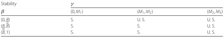
Table 3 The stability properties of the disease-free equilibrium point whene>E

Stability γ

β (0,M1) (M1,M2) (M2,M3)

(0,B) S. U. S. U. S.

(B,B) S. S. U. S.

(B, 1) S. S. U. S.

the conditions and conclusions of Theorem4.1–Theorem4.6are listed in Table1,Table2, and Table3in which

(1) S.means the disease-free equilibrium pointE2(S˜, 0,Y˜)is stable; (2) U.S.means the disease-free equilibrium pointE2(S˜, 0,Y˜)is unstable; (3) A.S.means the disease-free equilibrium pointE2(S˜, 0,Y˜)is always stable; (4) U.D.means the disease-free equilibrium pointE2(S˜, 0,Y˜)is undeﬁned.

Table1shows the stability properties of the disease-free equilibrium pointE2(S˜, 0,Y˜) whene<E.

Table2shows the stability properties of the disease-free equilibrium pointE2(S˜, 0,Y˜) whenE<e<E.

Table3shows the stability properties of the disease-free equilibrium pointE2(S˜, 0,Y˜) whene>E.

4.1.2 Global stability of the disease-free equilibrium

In this section, we consider the global stability of the disease-free equilibrium point E2(S˜, 0,Y˜).

Theorem 4.7 Ifβ>α¯(d1+ϕ(0)c2)Y˜

˜

S in whichα¯=α(1 –γ),then system(2.4)with initial

(8)

Proof We rewrite system (2.4) with initial conditions (2.3) as the following form:

˙

S(t) =SF1(S,I,Y),

˙

I(t) =IF2(S,I,Y),

˙

Y(t) =YF3(S,I,Y),

(4.5)

where

F1(S,I,Y) =r

1 – S+I (1 –γ)K

– βI

α(1 –γ) +I –c1Yϕ(S)/S,

F2(S,I,Y) =

βS

α(1 –γ) +I–d1–c2Yϕ(I)/I,

F3(S,I,Y) =ec1ϕ(S) +ec2ϕ(I) –d2.

Let us deﬁne

G1(I) = –F1(S¯,I,Y¯), G2(S) =F2(S, 0,Y¯), G3(Y) =F1(S¯, 0,Y) +F2(S¯, 0,Y).

Next, we consider a Lyapunov function deﬁned as follows:

VS(t),I(t),Y(t)= S

˜

S

G2(u) u du+

I

0 G1(v)

v dv+ Y

˜

Y

G3(w) w dw.

Now, by simple computation, we obtain that

dV

dt =G1F2(S,I,Y) +G2F1(S,I,Y) +G3F3(S,I,Y)

=G1F2(S,I,Y) –F2(S, 0,Y¯)+G2F1(S,I,Y) –F1(S¯,I,Y¯)+G3F3(S,I,Y)

+G2F1(S¯,I,Y¯) +G1F2(S, 0,Y¯)

+G3F1(S¯, 0,Y) –F1(S¯, 0,Y)

=G2

(S–S1)∂F1

∂S (S¯,I,Y) + (Y–Y1)

∂F1

∂Y(S,I,Y¯)

+G1

I∂F2

∂I (S,¯¯I,Y) + (Y–Y1)

∂F2

∂Y(S,I,Y¯¯)

+G3

(S–S1)∂F3

∂S(S¯¯¯,I,Y) +I

∂F3

∂I (S,I¯¯¯,Y)

.

Again, we have

∂F1

∂S = – r K –

c1Yϕ(S)S–ϕ(S) S2 < 0,

∂F1

∂Y = –c1ϕ(S) < 0,

∂F2

∂I = –

¯ αβS (α¯+I)2 –

c2Yϕ(I)I–ϕ(I) I2 < 0,

∂F2

∂Y = –c2ϕ(I) < 0,

∂F3

∂S =ec1ϕ

₍_S_{) > 0,} ∂F2

∂I =ec2ϕ

(9)

Furthermore, we obtain that

G1(I) = –

r

1 –S˜+I K

– βI

¯ α+I –

c1Y˜ϕ(S˜)

˜

S

> 0

and

G2(S) =βS

¯

α –d1–ac2Y˜≥ βS˜

¯

α –d1–ac2Y˜,

in whicha=limx→0ϕ(_xx)=ϕ(0).

Thus, it is obtained thatG2> 0 whileβ>α¯(d1+ϕ(0)c2)Y˜

˜

S .

Therefore, dV_dt < 0 in the region={(S,I,Y)|S≥ ˜S,I≥0,Y≥ ˜Y}. Hence the theorem is

proved.

4.2 Stability of the positive equilibrium

4.2.1 Local stability of the positive equilibrium

In this section, we consider the local stability of the positive equilibrium pointE3(S∗,I∗, Y∗).

Theorem 4.8 If A1< 0and A1A2<A3< 0,then the positive equilibrium point E3(S∗,I∗,Y∗) is locally asymptotically stable.

Proof The characteristic equation of the community matrix corresponding to the positive equilibrium pointE3(S∗,I∗,Y∗) is as follows:

λ3– (a11+a22)λ2+ (a11a22–a12a21–a13a31–a23a32)λ

– (a11a23a32+a13a31a22–a21a13a32–a12a23a31) = 0,

where

a11= –rS

∗

K –c1Y

∗_ϕ_S∗_–_ϕ_S∗_,

a12= –rS

∗

K –

αβ(1 –γ) ((1 –γ)α+I∗)2c1Y

∗_ϕ_S∗_–_ϕ_S∗_, _a13_{= –}_c1_ϕ_S∗_,

a21= βI

∗

(1 –γ)α+I∗,

a22=

αβ(1 –γ) ((1 –γ)α+I∗)2 –

βS∗

(1 –γ)α+I∗–c2Y

∗_ϕ_I∗_–_ϕ_I∗_,

a23= –c2ϕI∗,

a31=ec1Y∗ϕS∗, a32=ec2Y∗ϕI∗.

Now, deﬁne

A1=a11+a22, A2=a11a22–a12a21–a13a31–a23a32,

(10)

Therefore, the characteristic equation of the positive equilibrium pointE3(S∗,I∗,Y∗) can be rewritten as the following form:

λ3–A1λ2+A2λ–A3= 0.

According to Routh–Hurwitz’s criteria, the necessary and suﬃcient conditions for local stability of positive point areA1< 0 andA1A2<A3< 0. Hence the theorem is proved.

4.2.2 Global stability of the positive equilibrium

In this section, we consider the global stability of the positive equilibrium point E3(S∗,I∗,Y∗).

Theorem 4.9 System(2.4)with initial conditions (2.3)is to be globally asymptotically stable around the positive equilibrium point E3(S∗,I∗,Y∗)in the region2={(S,I,Y)|Y> Y∗, 0 <S<S∗, 0 <I<I∗orY<Y∗,S>S∗,I>I∗}.

Proof We ﬁrst choose a Lyapunov function which is deﬁned as follows:

WS(t),I(t),Y(t)=

Now, by simple computation, we obtain that

dW

(11)

The characteristic equation of system (2.4) at the disease-free equilibriumE2(S˜, 0,Y˜) is given by the following form:

λ3–A(γ) +B(γ)λ2+A(γ)B(γ) +C(γ)λ–A(γ)C(γ) = 0, (5.1)

where

A(γ) =βS˜

α –d1–c2(1 –γ)ϕ

₍₀₎_Y_˜_,

B(γ) =r

1 – 2S˜ (1 –γ)K

–c1(1 –γ)ϕ

(1 –γ)S˜Y˜,

C(γ) =c2₁e(1 –γ)ϕ(1 –γ)S˜ϕ(1 –γ)S˜Y˜ > 0.

It is noted that the expressionsA(γ),B(γ), andC(γ) are smooth functions ofγ. In order to determine the instability of system (2.4), let us considerγ (the eﬀect of prey refuge) as a bifurcation parameter. For this purpose, let us ﬁrstly give the following lemma.

Lemma 5.1(Hopf bifurcation theorem [16]) If A(γ),B(γ),and C(γ)are smooth functions ofγ in an open interval aboutγ ∈R,such that the characteristic equation(5.1)has

(1) a pair of complex eigenvaluesλ=p(γ)±iq(γ)withp(γ)andq(γ)∈R,so that they become purely imaginary atγ =γ0and dp_d(γγ)|(γ =γ0)= 0,

(2) the other eigenvalue is negative atγ =γ0,

then a Hopf bifurcation occurs around an equilibrium point of the considered system at

γ =γ0(i.e.,a stability change of an equilibrium point of the considered system accompanied by the creation of a limit cycle atγ=γ0).

Based on Lemma5.1, the following conclusion can be obtained.

Theorem 5.2 If A< 0and B< 0,then system(2.4)possesses a Hopf bifurcation around the

disease-free equilibrium E2(S˜, 0,Y˜).

Proof Suppose the valueγ0is equal to

1 –ϕ –1₍d2

ec1)

αK

_β_d2K₊_α_c2er_ϕ₍₀₎_ϕ–1₍d2

ec1) d1d2+c2erϕ–1(_ecd2₁)

,

or

1 –ϕ –1₍d2

ec1) K

₂_d2_–_ec1_ϕ₍_ϕ–1₍d2

ec1))ϕ –1₍d2

ec1) d2–ec1ϕ(ϕ–1₍d2

ec1))ϕ –1₍d2

ec1)

,

which are the roots ofA= 0 orB= 0, respectively.

Firstly, forγ =γ0, the characteristic equation of system (2.4) at the disease-free equilib-riumE2(S˜, 0,Y˜) becomes the following form:

(12)

It is clear that the roots of the above equation areλ1=A< 0,λ2=i

√

C, andλ1= –i

√

C. Hence, there exist a pair of purely imaginary eigenvalues and a strictly negative real eigenvalue.

Secondly, forγ in a neighborhood ofγ0, the roots have the formλ1=A< 0,λ2=p1(γ) + ip2(γ) andλ3=p1(γ) –ip2(γ) in whichp1(γ) andp2(γ) are real.

Next, we shall verify the transversality condition:

d dγ

Reλi(γ)

|(γ =γ0)= 0, i= 1, 2.

Substitutingλ2=p1(γ) +ip2(γ) into the characteristic Eq. (5.1), we get

p1(γ) +ip2(γ)3–A(γ) +B(γ)p1(γ) +ip2(γ)2+A(γ)B(γ)

+C(γ)p1(γ) +ip2(γ)–A(γ)C(γ) = 0. (5.2)

Taking derivatives of both sides of (5.2) with respect toγ, we have

3p1(γ) +ip2(γ) 2

p₁(γ) +ip₂(γ)–A(γ) +B(γ)p1(γ) +ip2(γ) 2

– 2A(γ) +B(γ)p1(γ) +ip2(γ)

p₁(γ) +ip₂(γ)

+A(γ)B(γ) +A(γ)B(γ) +C(γ)p1(γ) +ip2(γ)

+A(γ)B(γ) +C(γ)p₁(γ) +ip₂(γ)–A(γ)C(γ) –A(γ)C(γ) = 0. (5.3)

Comparing real and imaginary parts from both sides of Eq. (5.3), we obtain

3p2₁– 3p2₂– 2p1D1+D2p₁– (6p1p2– 2p2D1)p₂

+p1p2+P1D₂–P₁2D₁–D₃= 0,

(6p1p2– 2p2D1)p1–

3p2₁– 3p2₂– 2p1D1+D2

p₂+P2D2 – 2P1P1D1

= 0,

(5.4)

where

D1=A(γ) +B(γ), D2=A(γ)B(γ) +C(γ), D3=A(γ)B(γ).

DeﬁneE1= (3p2

1– 3p22– 2p1D1+D2),E2= (6p1p2– 2p2D1),E3= (p1p2+P1D2–P12D1–D3), andE4= (P2D₂– 2P1P1D₁), then Eqs. (5.4) become of the following form:

E1p₁–E2p₂+E3= 0,

E2p₁+E1p₂+E4= 0.

(5.5)

The value ofp1can be obtained by solving Eqs. (5.5)

p₁=E1E3+E2E4 E2

1+E21 .

Forp1= 0 and any other possible value ofp2atγ =γ0, theE1E3+E2E4is always unequal to zero since D2D3

3D3+2D1D2 =

(13)

Therefore,λ1=A< 0 and

d dγ

Reλi(γ)|(γ =γ0) =

E1E3+E2E4 E2

1+E21

= 0, i= 1, 2.

Hence, according to Lemma5.1, the theorem is proved.

6 Permanence

In this section, we prove the permanence of system (2.4) with initial conditions (2.3) under the conditionXϕ(X) <ϕ(X) (X> 0).

Deﬁnition 6.1([6]) If there exist positive constantsmS,MS,mI,MI,mY, andMY such

that each solution (S(t),I(t),Y(t)) of system (2.4) satisﬁes

0 <mS≤lim inf

t→+∞ S(t)≤lim supt→+∞ S(t)≤MS,

0 <mI≤lim inf

t→+∞ I(t)≤lim supt→+∞ I(t)≤MI,

0 <mY≤lim inf

t→+∞ Y(t)≤lim sup_t_→+∞ Y(t)≤MY,

then system (2.4) is permanent. Otherwise, it is non-permanent.

In order to consider the permanence of system (2.4), we consider the following auxiliary system:

˙

S(t) =rS

1 –S+I K

– βSI

α+A–c1BS,

˙

I(t) = βSI

α+C–dI–c2DI,

(6.1)

in whichA,C, andDare non-negatively constant numbers,Bis positive and bounded by

r c1.

For system (6.1), we can obtain the following result.

Lemma 6.2 The positive equilibrium point of system(6.1)is globally asymptotically stable when it exists.

Proof The positive equilibrium point of system (6.1) isP¯(S¯,¯I), where

¯

S=(α+C)(d+c2D)

β , ¯I=

K(r–c1B) –rS¯ r(α+A) +βK .

The equilibrium pointP¯(S¯,¯I) is positive ifβ>r(α+C)(d+c2D)

K(r–c1B) . The Jacobian matrix of system (6.1) atP¯(S¯,¯I) is

J=

–rS¯

K –

(r(α+A)+βK)S¯ K(α+A) β¯I

α+C 0

.

(14)

Therefore, the positive equilibrium pointP¯(S¯,¯I) is locally asymptotically stable. Next, we show its global asymptotic stability.

We consider the following function:

V=

S–S¯–S¯lnS

¯

S

+E

I–I¯–I¯lnI

¯

I

.

From the construction of V, it is easily seen thatV is positive deﬁnite in the region

={(S,I)|S≥0,Y≥0}andV(S¯,¯I) = 0. By simple computation, we obtain that

dV dt =

S–S¯ S S(˙t) +

I–I¯ I S(˙I)

= –r(S–S¯) 2

K +

βE

α+C– r K –

β α+A

(S–S¯)(I–I¯).

LetE=(α+C_β)(_Kr(₍α_α+₊A_A)+₎βK)> 0, then dV_dt ≤0 in the region={(S,I)|S≥0,Y≥0}.

Hence the theorem is proved.

Next, we consider the permanence of system (2.4) with initial conditions (2.3).

Theorem 6.3 Ifβ>r(α+(1–γ)K)(d1+c2ϕ(0)MY)

(1–γ)K(r–c1ϕ(0)MY) > 0and0 <MY < r

c1ϕ(0),then system(2.4)with initial conditions(2.3)is permanent.Otherwise,it is non-permanent.

Proof From the ﬁrst and second equations of system (2.4), we obtain that

˙

S(t)≤rS

1 – S+I (1 –γ)K

– βSI

(1 –γ)α+K, ˙I(t)≤

βSI

(1 –γ)α–d1I.

By Lemma6.2and a standard comparison theorem, we have

lim sup

t→+∞

S(t)≤ ˆS=. MS, lim sup t→+∞

I(t)≤ ˆI=. MI,

whereSˆ=αd1(1–γ) β > 0,ˆI=

((1–γ)α+K)((1–γ)rK–Sˆ)

(1–γ)(rα+βK)+K > 0 ifβ>

αd1

rK.

Thus, for any givenε> 0, there existsT1> 0 such that, for anyt>T1> 0, we get

S(t)≤MS+ε, I(t)≤MI+ε.

From the third equation, we obtain that

˙

Y(t)≤ec1ϕ(MS+ε)

+ec2ϕ(MI+ε)

–d2Y.

It is easy to show that there isMY> 0 such that

lim sup

t→+∞ Y(t)≤MY.

Hence, for any givenε> 0, there existsT2>T1> 0 such that, for anyt>T2> 0, we have

(15)

Again, from the ﬁrst and second equations, we get

˙

S(t)≥rS

1 –S+I K

–βSI

α –c1M(MY+ε)S,

˙

I(t)≥ βSI

α+K –d1I–c2M(MY+ε)I,

whereMis the maximum value of the functionF(X), where

F(X) = ⎧ ⎨ ⎩

ϕ(X)/X (0 <X≤K),

ϕ(0) (X= 0). (6.2)

Notice that the functionF(X) has the maximum and minimum values since it is contin-uous on the closed interval [0,K].

By Lemma6.2and a standard comparison theorem, we have

lim inf

t→+∞ S(t)≥S ∗₌. _m

S, lim inf

t→+∞ I(t)≥I ∗₌. _m

I,

where

S∗=(α+ (1 –γ)K)(d1+c2ϕ

₍₀₎_M

Y)

β > 0, I

∗₌(1 –γ)K(r–c1ϕ(0)MY) –rS∗ αr+ (1 –γ)βK > 0,

whenβ>r(α+(1–γ)K)(d1+c2ϕ(0)MY)

(1–γ)K(r–c1ϕ(0)MY) > 0 and 0 <MY< r c1ϕ(0).

Thus, for any givenε> 0, there existsT3>T2>T1> 0 such that, for anyt>T3> 0, we obtain

S(t)≥mS–ε, I(t)≥mI–ε.

Again, from the third equation, we get

˙

Y(t)≥ec1ϕ

(1 –γ)(mS–ε)

+ec2ϕ

(1 –γ)(mI–ε)

–d2

Y.

It is easy to show that there ismY> 0 such that

lim inf

t→+∞ Y(t)≥mY> 0.

According to Deﬁnition6.1, system (2.4) with initial conditions (2.3) is permanent under

some strict conditions. Hence the theorem is proved.

7 Examples

Example1 Ifϕ(X) = _aX₊_X, then system (2.2) becomes the following system:

˙

S(t) =rS

1 –S+I K

– βSI

α+I –

c1(1 –γ)XY a+ (1 –γ)X,

˙

I(t) = βSI

α+I–d1I–

c2(1 –γ)IY a+ (1 –γ)I,

˙

Y(t) =ec1(1 –γ)XY a+ (1 –γ)X +

ec2(1 –γ)IY a+ (1 –γ)I –d2Y.

(16)

It is easy to obtain the disease-free equilibrium pointE1(S1, 0,Y1) of system (7.1), where

By simple computation, the equilibrium pointE1(S1, 0,Y1) has its ecological meanings if

γ < 1 – ad2

K(c1e–d2).

According to the theorems in Sect.4, we can obtain the following propositions:

(1) Assuming thatαd1

equilibrium point of system (7.1) is locally asymptotically stable; (c) If1 – ad2(αc2er+βK(c1e–d2))

αK(c1e–d2)(c2er+d1(c1e–d2))<γ < 1 –

ad2

K(c1e–d2), then the disease-free equilibrium

point of system (7.1) is unstable. (2) Assuming thatβ<αd1

K , then the disease-free equilibrium point of system (7.1) is

always locally asymptotically stable.

S2= 1

(1) Assuming thatαd1

c1e–d2, then the disease-free equilibrium point of system

(7.2) is unstable;

c1e–d2, then the disease-free equilibrium

point of system (7.2) is locally asymptotically stable; (c) If1 –_αβ_d

c1e–d2, then the disease-free equilibrium point of

system (7.2) is unstable. (2) Assuming thatβ<αd1

(7.2) is unstable;

(17)

Example3 Ifϕ(X) = _aX₊_Xpp, then system (2.2) becomes the following system:

S3= 1

(I) Supposing thatαd1

point of system (7.3) is unstable; (b) If1 –_K1p ad2

equilibrium point of system (7.3) is locally asymptotically stable; (c) If1 –_αβ_d

point of system (7.3) is unstable. (2) Assuming thatp> 2c1e

point of system (7.3) is locally asymptotically stable; (b) If1 –_K1p ad2

equilibrium point of system (7.3) is unstable. (3) Assuming that c1e

(7.3) is locally asymptotically stable; (b) If1 –_αβ_d

point of system (7.3) is unstable. (II) Supposing thatβ<αd1

point of system (20) is unstable; (b) If1 –_K1p ad2

equilibrium point of system (20) is locally asymptotically stable. (2) Assuming thatp> 2c1e

(18)

(b) If1 –_K1p ad2

c1e–d2[

2c1e–p(c1e–d2)

c1e–p(c1e–d2)] <γ< 1 – 1

K p

ad2

c1e–d2, then the disease-free

equilibrium point of system (20) is unstable. (3) Assuming that c1e

c1e–d2 <p< 2c1e

c1e–d2, then the disease-free equilibrium point of

system (20) is always locally asymptotically stable.

8 Discussion

In this paper, a generalized system describing predator–prey interaction with prey refuges and disease in prey is proposed. Based on mathematical issues, the dynamical properties (stability, Hopf bifurcation, and permanence) are investigated, and the sufficient condi-tions which guarantee these properties are obtained (see Sects.4,5,6). However, based on ecological and epidemiological issues, our analyses reveal that the effect of prey refuge, the force of infection, and the converting efficiency of predators play an important role in the dynamical properties of the proposed system. The ecological and epidemiological meanings will be discussed according to the following aspects:

(1) If the infectious rate of prey is smaller than the thresholdB, then the effect of prey refuge has a stabilizing impact when the converting ratio is relatively small. The contrary effect happens under the larger converting ratio for predators. However, the effect of prey refuge has no influence under the middle converting ratio and the disease will vanish. These results show that the infectious disease can be prevented by controlling the degree of the effect of prey refuge under the certain converting ratio.

(2) If the infectious rate of prey is larger than the thresholdB, the dynamical consequences of the considered system will be relatively simple. In this case, in order to control the infectious disease which will break out, the eﬀect of prey refuge must be relatively small.

(3) If the infectious rate is smaller thanBand larger thanB, the stabilizing effect and destabilizing effect will occur under the small converting ratio, and the destabilizing effect happens while the converting ratio is larger than the thresholdB. Therefore, for the small converting ratio, the middle level of prey refuge can be applied to control the infectious disease. But, for the larger converting ratio, the smaller level of prey refuge is required to control the disease.

(19)

strategy and the evolutionary strategy of predator population are the main factors which induce the partially hiding behavior (prey refuge) of prey population.

On the other hand, our results show that the eﬀect of prey refuge can be applied to control the spread of the infectious disease. The level of prey refuge needed to control the disease spread is mainly determined by the infectious rate and the converting ratio of predators.

Acknowledgements

All authors would like to thank the editor and the anonymous referees for their valuable comments and suggestions.

Funding

This work was supported by the Fundamental Research Funds for the Central Universities of Northwest Minzu University (No. 31920180116), Gansu Provincial ﬁrst-class discipline program of Northwest Minzu University, the Fundamental Research Funds for the Central Universities (No.lzujbky-2017-166) and the National Natural Science Foundation of China (No. 31560127).

Competing interests

The authors declare that they have no competing interests.

Authors’ contributions

All authors contributed equally and signiﬁcantly in this paper. All authors read and approved the ﬁnal manuscript.

Author details

1_{School of Mathematics and Computer Science, Northwest University for Nationalities, Lanzhou, China.}2_{School of}

Mathematics and Statistics, Lanzhou University, Lanzhou, China.

Publisher’s Note

Springer Nature remains neutral with regard to jurisdictional claims in published maps and institutional aﬃliations.

Received: 13 November 2017 Accepted: 1 July 2018 References

1. Anderson, R.M., May, R.M.: The invasion, persistence and spread of infectious diseases within animal and plant communities. Philos. Trans. R. Soc. Lond. B314, 533–570 (1986)

2. Hadeler, K.P., Freedman, H.I.: Predator-prey populations with parasite infection. J. Math. Biol.27, 609–631 (1989) 3. Xiao, Y., Tang, S.: Dynamics of infection with nonlinear incidence in a simple vaccination model. Nonlinear Anal., Real

World Appl.11, 4154–4163 (2010)

4. Chattopadhyay, J., Arino, O.: A predator-prey model with disease in the prey. Nonlinear Anal., Theory Methods Appl.

36, 747–766 (1999)

5. Chattopadhyay, J., Bairagi, N.: Pelicans at risk in Salton Sea|an eco-epidemiological study. Ecol. Model.136, 103–112 (2001)

6. Venturino, E.: Epidemics in predator-prey models: disease in the predator. IMA J. Math. Appl. Med. Biol.19, 185–205 (2002)

7. Hethcote, H.W., Wang, W., Han, L., Ma, Z.: A predator-prey model with infected prey. Theor. Popul. Biol.66, 259–268 (2004)

8. Hall, S.R., Dufy, M.A., Caceres, C.E.: Selective predation and productivity jointly drive complex behavior in host-parasite systems. Am. Nat.165, 70–81 (2005)

9. Fenton, A., Rands, S.A.: The impact of parasite manipulation and predator foraging behavior on predator-prey communities. Ecology87, 2832–2841 (2006)

10. Bairagi, N., Roy, P.K., Chattopadhyay, J.: Role of infection on the stability of a predator-prey system with several functional responses—A comparative study. J. Theor. Biol.248, 10–25 (2007)

11. Bhattacharyya, R., Mukhopadhyay, B.: On an eco-epidemiological model with prey harvesting and predator switching: local and global perspectives. Nonlinear Anal., Real World Appl.11(455), 3824–3833 (2010) 12. Bob, W., George, A.K., Krishna, D.: Stabilization and complex dynamics in a predator-prey model with predator

suﬀering from an infectious disease. Ecol. Complex.8, 113–122 (2011)

13. Saifuddin, M., Biswas, S., Samanta, S., Sarkar, S., Chattopadhyay, J.: Complex dynamics of an eco-epidemiological model with diﬀerent competition coeﬃcients and weak Allee in the predator. Chaos Solitons Fractals91, 270–285 (2016)

14. Biswas, S., Samanta, S., Chattopadhyaya, J.: A model based theoretical study on cannibalistic prey-predator system with disease in both populations. Diﬀer. Equ. Dyn. Syst.23, 327–370 (2015)

15. Biswas, S., Sasmal, K.S., Samanta, S., Saifuddin, M., Khan, Q.J.A., Alquranc, M.: A delayed eco-epidemiological system with infected prey and predator subject to the weak Allee eﬀect. Math. Biosci.263, 198–208 (2015)

16. Liu, X.: Bifurcation of an eco-epidemiological model with a nonlinear incidence rate. Appl. Math. Comput.218, 2300–2309 (2011)

17. Holling, C.S.: Some characteristics of simple types of predation and parasitism. Can. Entomol.91, 385–398 (1959) 18. Ma, Z., Li, W., Zhao, Y., Wang, W., Zhang, H., Li, Z.: Eﬀects of prey refuges on a predator-prey model with a class of

(20)

19. Ma, Z., Wang, S., Wang, T., Tang, H.: Stability analysis of prey-predator system with Holling type functional response and prey refuge. Adv. Diﬀer. Equ.2017, 243 (2017)

20. Ruxton, G.D.: Short term refuge use and stability of predator-prey models. Theor. Popul. Biol.47, 1–17 (1995) 21. Gonzalez-Olivars, E., Ramos-Jiliberto, R.: Dynamics consequences of prey refuges in a simple model system: more

prey, few predators and enhanced stability. Ecol. Model.166, 135–146 (2003)

22. Hassel, M.P., May, R.M.: Stability in insect host-parasite models. J. Anim. Ecol.42, 693–725 (1973) 23. Smith, J.M.: Models in Ecology. Cambridge Univ. Press, Cambridge (1974)

24. Murdoch, W.W., Stewart-Oaten, A.: Predation and population stability. Adv. Ecol. Res.9, 1–13 (1975) 25. Hassell, M.P.: The Dynamics of Arthropod Predator-Prey Systems. Princeton Univ. Press, Princeton (1978) 26. Sih, A.: Prey refuges and predator-prey stability. Theor. Popul. Biol.31, 1–12 (1987)

27. Ives, A.R., Dobson, A.P.: Antipredator behavior and the population dynamics of simple predator-prey systems. Am. Nat.130, 431–447 (1987)

28. Hochberg, M.E., Holt, R.D.: Refuge evolution and the population dynamics of coupled host-parasitoid associations. Evol. Ecol.9, 633–661 (1995)

29. Michalski, J., Poggiale, J.C., Arditi, R., Auger, P.M.: Macroscopic dynamic eﬀects of migration in patchy predator-prey systems. J. Theor. Biol.185, 459–474 (1997)

30. Krivan, V.: Eﬀects of optimal antipredator behavior of prey on predator-prey dynamics: the role of refuges. Theor. Popul. Biol.53, 131–142 (1998)

31. Ghosh, J., Sahoo, B., Poria, S.: Prey-predator dynamics with prey refuge providing additional food to predator. Chaos Solitons Fractals96, 110–119 (2017)

32. Kar, T.K.: Stability analysis of a prey-predator model incorporating a prey refuge. Commun. Nonlinear Sci. Numer. Simul.10, 681–691 (2005)

33. Hoy, M.A.: Almonds (California). In: Helle, W., Sabelis, M.W. (eds.) Spider Mites: Their Biology, Natural Enemies and Control, World Crop Pests. 1B. Elsevier, Amsterdam (1985)

34. Huang, Y., Chen, F., Zhong, L.: Stability analysis of a prey-predator model with Holling type III response function incorporating a prey refuge. Appl. Math. Comput.182, 672–683 (2006)

35. May, R.M.: Stability and Complexity in Model Ecosystems. Princeton University Press, Princeton (1974) 36. McNair, J.M.: The eﬀects of refuges on predator-prey interactions: a reconsideration. Theor. Popul. Biol.29, 38–63