Improved Simultaneous Estimation of Location and System Reliability via Shrinkage Ideas

(1)

University of South Carolina

Scholar Commons

Theses and Dissertations

5-2017

Bayesian Flexible Modeling of Interval-censored

Failure Time Data

Sheng-Yang Wang

University of South Carolina

Follow this and additional works at:https://scholarcommons.sc.edu/etd Part of theStatistics and Probability Commons

This Open Access Dissertation is brought to you by Scholar Commons. It has been accepted for inclusion in Theses and Dissertations by an authorized administrator of Scholar Commons. For more information, please [email protected].

Recommended Citation

(2)

Bayesian Flexible Modeling of Interval-censored Failure Time Data

by

Sheng-Yang Wang

Bachelor of Science TamKang University, 1995

Master of Science

The University of New Mexico, 2009

Master of Science

The University of New Mexico, 2011

Submitted in Partial Fulfillment of the Requirements

for the Degree of Doctor of Philosophy in

Statistics

College of Arts and Sciences

University of South Carolina

2017

Accepted by:

Lianming Wang, Major Professor

John Grego, Committee Member

David Hitchcock, Committee Member

Yi Sun, Committee Member

(3)

c

Copyright by Sheng-Yang Wang, 2017

(4)

Acknowledgments

I would like to thank Dr. Lianming Wang sincerely. I appreciate for his

encourage-ment, training, and advice for the necessary courses and knowledge required for this

research.

I give special thanks to Dr. Grego for his incisive comments on my dissertation

context. In addition, he helped me develop my statistical consulting experience in

my career. I also thank to my committee members, Dr. Hitchcock and Dr. Sun for

their insightful comments and suggestions in supporting my dissertation.

At last, not the least, I dedicate this work to my beloved wife, Esther, who has

shown so much confidence in me and has given me great encouragement with her

unconditional love and patient. Without her accompanying in the journey, I cannot

move the important step to complete my Ph.D. In addition, I am proud of my lovely

and cute children, Emunah and Emeth for their mature mindsets above their own

age to fully support me over the past few years all the time.

As a believer in Jesus Christ, I thank my Lord and Savior, Jesus Christ, for His

work on me through my graduate study and research. As it is said in the Bible,

"Although the Lord gives you the bread of adversity and the water of affliction, your

teacher will be hidden no more; with your own eyes you will see them. Whether you

turn to the right or to the left, your eyes will hear a voice behind you, saying, ’This

(5)

Abstract

Interval-censored data are a special type of survival data, in which the survival time

is not accurately observed but known to fall within a specific time interval.

Interval-censored data commonly arise in real-life epidemiological and medical studies that

involve periodic examinations. In this dissertation, several semiparametric regression

models are investigated to provide flexible modeling and robust inference for

interval-censored data from Bayesian perspectives.

Chapter 1 provides a detailed description about interval-censored data and gives

several examples. Existing models and methods for analyzing such interval-censored

data are reviewed as well. Chapter 2 develops a unified Bayesian estimation approach

under the framework of semiparametric linear transformation models for regression

analysis of current status data, which is a special type of interval-censored data. This

work provides an alternative estimation approach to the existing methods for the

proportional hazards, proportional odds, and probit models. As a unified Bayesian

estimation approach, the proposed method allows direct comparison of three

differ-ent semiparametric regression models in the same framework of the Gibbs Sampler.

Chapter 3 proposes a Bayesian estimation approach for analyzing general

interval-censored data under the generalized odds-rate hazards (GORH) models. The GORH

models are a general class of semiparametric regression models including the

propor-tional hazards and proporpropor-tional odds models as special cases. Submodels of GORH

models can be specified by indexing a non-negative value ν, where the "sub" prefix

refers to the fact that for each ν, a semiparametric regression model is well-specified

(6)

an unknown parameter leads to biased estimation, which in this case is a consistent

research result for right-censored data in the literature. To solve this issue, a Bayesian

approach with a known ν is proposed and has shown excellent performance in the

simulation study. Chapter 4 extends the semiparametric probit model for regression

analysis of arbitrarily censored data. The proposed method has been implemented

using two sets of latent variables for posterior computation. The proposed method

can be easy to implement in the estimation of regression parameters for two special

types of arbitrarily censored data: right-censored data and general interval-censored

(7)

List of Tables

Table 2.1 Sensitivity Analysis: Estimation of the regression coefficients for

different hyper-parameters,aλandbλ based on 200 simulated datasets. 33

Table 2.2 Mean square errors of the estimates ofF0 based on 200 datasets. . 34

Table 2.3 Model Comparison of LPML criteria based on 200 datasets. . . 35

Table 2.4 The optimal knots of three candidate models for estimating a

non-parametric transformation function. The comparison of the Log Pseudo Marginal Likelihood (LPML) value in uterine

fi-broids data analysis. . . 36

Table 2.5 Results of fibroids data analysis: Posterior Mean (Mean) and

95% Credible Interval (CI) of fibroids when applying equispaced

knots and degree 3 for monotone spline for three proposed models. 37

Table 3.1 Estimation of the regression parameters (β1, β2) based on 100

simulated datasets. . . 57

Table 3.2 Sensitivity Analysis: the estimated regression coefficients (β1, β2)

for a Gamma hyper prior with parameters (aη, bη) = (0.1,0.1). . . 58

Table 3.3 Sensitivity Analysis: the estimated regression coefficients (β1, β2)

for a Gamma hyper prior with parameters (aη, bη) = (0.01,0.01). . 59

Table 3.4 The estimated covariate effects and their corresponding 95%

Credible Intervals from the proposed approach using quadratic and cubic splines and the number of knots 10 in the analysis of

HIV data. . . 60

Table 3.5 Regression parameter estimates and their associated estimated

standard error and 95% credible interval under GORH models by using quadratic basis function with 30 equally spaced knots

(10)

Table 4.1 Estimation of regression coefficients (β1, β2) based on 100 sim-ulated datasets, sample size 200 per se, basis spline function

degree 3 and interior knots 5. . . 80

Table 4.2 Maximumlikelihood method for the estimation of regression

co-efficients (β1, β2) based on 100 simulated datasets, sample size

200 per se, basis spline function degree 3 and interior knots 5. . . . 81

Table 4.3 Bayesian method for the estimation of the regression parameters

(β1, β2) based on 100 simulated datasets, sample size 200 per se,

basis spline function degree 4 and interior knots 10. . . 82

Table 4.4 Maximumlikelihood method for the estimation of the regression

coefficients (β1, β2) based on 100 simulated datasets, sample size

200 per se, basis spline function degree 4 and interior knots 10. . . 83

Table 4.5 Simulation results of three different levels of the completely

ob-served rate dataset for concerning the estimation on the baseline

cumulative distribution function F0. Provided results include

the average (MSE) and maximum (maxMSE) mean squared errors

(×10−3_{) of the estimates of the baseline cumulative distribution}

functionF0(t) calculated over a set of pre-specified time points.

Modeling the nonparametric transformation function is based on

Table 4.6 Simulation results of three different levels of the completely

ob-served rate dataset for concerning the estimation on the baseline

cumulative distribution function F0. Provided results include

the average (MSE) and maximum (maxMSE) mean squared errors

(×10−3_{) of the estimates of the baseline cumulative distribution}

functionF0(t) calculated over a set of pre-specified time points.

Modeling the nonparametric transformation function is based on

Table 4.7 Estimation of the regression parameters (β1, β2) based on 100

simulated datasets, sample size 200 per se for right-censored data. 86

Table 4.8 Summary characteristics for Steno Memorial Hospital Diabetic

Nephropathy data . . . 87

Table 4.9 Estimated covariate effects on the DN incidence from the

pro-posed method under the PB model and from the likelihood

(11)

List of Figures

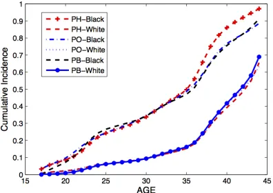
Figure 2.1 Estimated cumulative incidences functions for African and white

American women under three difference semiparametric

regres-sion models. . . 38

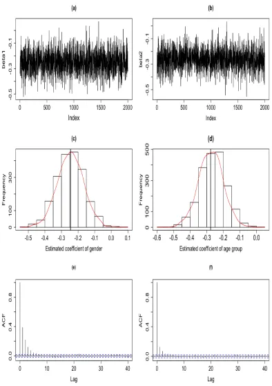
Figure 4.1 SMH diagnosis plots: Trace plot of ˆβ1 (a), Trace of ˆβ2 (b),

Histogram of ˆβ1 (c), Histogram of ˆβ2 (d), Autocorrelation of ˆβ1

(e), and Autocorrelation of ˆβ2 (f). . . 89

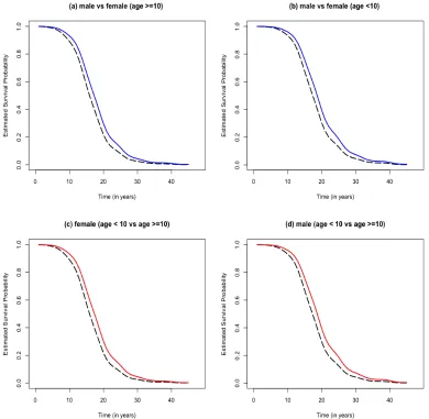
Figure 4.2 SMH data analysis: Estimates of the survival functions

ob-tained by the proposed method (smooth red curves) at the dif-ferent levels of gender and age group: Male vs. Female partici-pants between ages 10 and 30 (a), Male vs Female participartici-pants under age 10 (b), Female participants under age 10 versus be-tween ages 10 and 30 (c), and Male participants under age 10 versus between ages 10 and 30 (d). Smooth blue curves are the indicators for Male (a) and (b). Smooth red curves are the

indicators for participants age under 10 (c) and (d). . . 90

Figure 4.3 SMH data analysis: Estimates of the survival functions

ob-tained by the proposed method (smooth red curves) and the Turnbull estimates (black step functions) at the different levels of gender and age group: Male participants above age 10 (a), Male participants under ages 10 (b), Female participants above

(12)

Chapter 1 Introduction

1.1 Interval-Censored Data

Observations in time-to-event data are subject to censoring when practitioners cannot

know or exactly observe the occurrence of an event. The failure time is usually

defined as the length of time until the occurrence of an event. Many clinicians and

epidemiologists have designed and conducted their experiments in prospective cohort

studies or longitudinal studies. In such studies, participants are often seen at

pre-scheduled visits or regular check-ups or random examinations but the event of interest

(e.g. failure) may occur in between visits. Interval-censored data naturally arise when

each subject is observed at only one time or inspected at a one-time sacrifice. For

example, in animal carcinogenicity studies, the onset of tumor cannot be known, but

the presence of tumors can be diagnosed through a biopsy or some laboratory test

in regular check-ups. Then the onset of tumor can be known to lie in a specific

time interval. In the literature, this type of censored data is so-called current status

data (a.k.a. case 1 interval-censored data) in time-to-event history data (Sun, 2007).

Interval-censored data naturally arise when each subject proceeds a periodic check-ups

or random examinations, for example, animal carcinogenicity studies and longitudinal

studies. In the literature, this type of censored data is so-called interval-censored data

(a.k.a. case 2 interval-censored data) in time-to-event history data (Groeneboom and

Wellner, 1992; Huang and Wellner, 1997; Kalbfleisch and Prentice, 2002; Sun, 2007).

(13)

time points. The failure can be known to occur before the first observation time,

between two adjacent observation times, or after the last observation time. For

example, the onset time of HIV for a participant is usually interval censored and the

observed interval is formed by the last examination time with negative status and

the first examination time with positive status for that participant. The structure

of interval-censored data accommodates the incidence of drop-outs. For example,

drop-outs occur when participants drop out or die before the end of the study or miss

several check-ups in the study, as in the breast cosmesis dataset (Finkelstein, 1986).

Current status data are a special case of interval-censored data. Current status

data are yielded when a periodic scientific investigation is limited to one random

examination for a diagnosis of whether or not the failure has been revealed. If failure

is revealed, the observation is left-censored; otherwise, right-censored. Current status

data are relatively more cost-effective and less time-consuming. The costs of studies

are often reduced by alleviating the frequency of observation times.

1.2 Motivating Examples

1.2.1 Uterine Leiomyomas Data

Right From the Start (RFTS) is an on-going, prospective cohort study of

early-pregnancy health that was conducted in three states (NC/TX/TN). In this cohort

study, the onset time of uterine fibroids was unknown. However, the onset time

of uterine fibroids was known to occur either before or after a one-time ultrasound

examination that was performed at the exact enrollment time of each participant, in

early pregnancy (prior to the seventh gestational week). Participants were diagnosed

as positive when the ultrasound examination revealed leiomyomata diameter of 0.5

cm or larger. A more detailed description of this study is available from (Laughlin

(14)

1.2.2 Prostate, Lung, Colorectal and Ovarian (PLCO) Cancer Screening

Trial Data

The Prostate, Lung, Colorectal, and Ovarian (PLCO) Cancer Screening Trial

spon-sored by the U.S. National Cancer Institute (NCI) is a multicenter and

random-ized two-arm trial designed to assess the effect of a regular screening strategy for

cancer-related mortality. This program was initiated in November 1993 and ended

in September 2001. Our analysis takes account of the prostate cancer screening data

collected on male participants in the intervention arm. The response variable of this

study is the time to onset of prostate cancer. The onset time of prostate cancer is

not observed, but is known to lie in two adjacent screenings because of the design of

the study and the diagnosis mechanism of prostate cancer. Two adjacent screenings

form one screening interval, and practitioners identify whether the onset of a tumor

exists or not through laboratory testing. Thus, the censoring information of each

subject can be obtained from a state of having a negative result in the previous test

and a state of having a positive result at the current one. Two other cases could be:

Participants have been diagnosed as positive at the enrollment time, or they could

have negative results in all screenings in the program. Thus, the PLCO data are

the interval-censored data. The primary goal of the present study is to estimate the

association of risk factors from the intervention arm with the onset of prostate

can-cer. For a more detailed description of this screening trial, please see Andriole et al.

(2012).

1.2.3 Diabetic Nephropathy

Diabetes mellitus is a common chronic disease caused due to a disturbance of

nor-mal production of insulin. There are two types of diabetes: Type 1 diabetes (a.k.a.

insulin-dependent or juvenile-onset) and Type 2 diabetes(a.k.a. non-insulin-dependent

(15)

pa-tients at a young age, and Type 2 diabetes is a mild type and develops in those

patients later in life. Nowadays, there are many obese children in the adolescent

population; therefore, there are many young people with insulin resistance and Type

2 diabetes. Moreover, the characteristics of both Type 1 and Type 2 diabetes may be

present in the same patient. Type 1 and Type 2 diabetes are difficult to distinguish.

The Steno Memorial Hospital in Copenhagen, Denmark served as a diabetes

re-search hospital beginning in 1933. A study was conducted there between 1933 and

1972 of patients who had been diagnosed before age 31 with insulin-dependent

di-abetes mellitus for Type 1 didi-abetes (Andersen et al., 1983). Borch-Johnsen et al.

(1985)’s research showed that the development of diabetic nephropathy (DN) was

regarded as a highly associated prognostic biomarker for a low survival rate in Type

1 diabetics. Insulin treatment was adopted as the primary method to treat diabetes

disease in 1922, but it is still possible for a patient treated with insulin to develop DN

for Type 1 diabetes. DN is defined as persistent proteinuria and not an irreversible

complication. It is mainly used to assess kidney failure, which is indicated as positive

whenever a subject has at least four urine samples within 24 hours, during a time

interval of at least one month, that each contain more than 0.5-gram of protein. The

survival time is used as the basic time scale from onset of a patient’s diabetes to the

time when they transition from having diabetes without DN to having diabetes with

DN. Subjects are diabetic patients who either enter this study with DN or develop

DN before the end of the study. The primary research interest is to estimate the

association of risk factors (e.g. gender and age at the onset of diabetes) with the

onset of the development of DN.

1.3 Literature Review

The primary research interests focus on the estimation of regression parameters and

(16)

1.3.1 Survival Curves

Without covariates, many existing approaches have been developed and applied to

estimate the survival curve for interval-censored data. For example, Peto (1973)

pro-posed the Newton-Raphson method to estimate the (experimental) survival curve.

Turnbull (1976) presented the self-consistent estimation algorithm, and Groeneboom

and Wellner (1992) introduced the iterative convex minorant (ICM) algorithm to

compute the nonparametric maximum likelihood estimator (NPMLE) for the

dis-tribution of failure time. Wellner and Zhan (1997) developed a hybrid algorithm

to facilitate the expectation-maximization (EM) algorithm and the ICM algorithm

to attain global convergence. Groeneboom and Wellner (1992)’s empirical studies

showed that using the ICM algorithm to estimate NPMLE converges faster than

Turnbull’s algorithm. Turnbull’s self-consistency algorithm is simple to implement,

though. Wellner and Zhan (1997)’s simulation studies reported that their algorithm

converges to the NPMLE faster than both the EM and ICM algorithms, with fewer

iterations and less computation time required for current status data. Moreover,

Wellner and Zhan (1997) emphasized that self-consistency equations do not

deter-mine the uniqueness of the NPMLE for interval-censored data. Finally, Gentleman

and Geyer (1994) proved that the Karush-Kuhn-Tucker conditions are necessary and

sufficient for optimization for a self-consistency procedure to apply standard convex

optimization techniques.

1.3.2 Regression Analysis

Almost at the same time as researchers were estimating the survival curve, many

approaches were developed for regression analysis of interval-censored data under

semiparametric survival models. For example, the proportional hazards (PH) model

(Cox, 1972, 1975), the proportional odds (PO) model (Bennett, 1983), and the probit

(17)

In the PH model, Andersen and Gill (1982) exploited counting process and

mar-tingale theory to provide an elegant proof for asymptotic normality of a consistent

maximum likelihood estimator for the right-censored data. Finkelstein (1986),

how-ever, commented that the martingale techniques cannot be adapted to current

sta-tus data because of the difficulty in defining an appropriately increasing sequence

of sigma-algebras. Many existing approaches have been developed to estimate the

regression coefficients. Huang (1996) demonstrated that the MLE of the finite

di-mensional regression parameter in the PH model is asymptotically efficient but the

infinite-dimensional parameter converges slower than √n for current status data.

Pan (1999) extended the iterative convex minorant algorithm, which was developed

by Groeneboom and Wellner (1992), to consider covariate effects in the PH model,

and this method is called the generalized gradient projection (GGP) method.

Spline-based methods have prevailed since the early 1990s for current status data analysis.

Kooperberg and Clarkson (1997) introduced hazard regression, and Kooperberg et al.

(1995) used linear splines and their tensor products in the estimation of the

condi-tional log-hazard function for interval-censored data. Shiboski (1998) fitted the

gen-eralized additive model (GAM) and isotonic regression, and provided simultaneous

estimation of regression coefficients and the baseline event time distribution. Cai and

Betensky (2003) proposed a flexible locally parametric procedure to model the

base-line log-hazard function and to obtain MLE via Penalized Spbase-line for interval-censored

data. Wang et al. (2015) developed a novel EM algorithm for regression analysis of

bivariate case 1 interval-censored data under the Gamma-frailty PH model. Wang

et al. (2016) developed a novel EM algorithm under the PH model. Compared to

frequentist approaches, Bayesian methods are few. For example, Cai et al. (2011)

proposed a Bayesian approach by using monotone splines.

Frequentist approaches for the PO model have also been introduced. Rossini and

(18)

the baseline function and the number of jumps in their methods, which are

prede-termined by a Lipschitz-continuity assumption. Huang and Rossini (1997) and Shen

(1998) developed a random sieve likelihood method on both the baseline function

and the regression coefficients. Chen et al. (2007) developed a maximum likelihood

approach to fit the marginal PO model for multivariate interval-censored data.

The accelerated failure time (AFT) model presumes that the logarithm of the

failure time is linearly related to the covariates, but also needs to take account of an

unspecified random error (Cox and Oakes, 1984; Kalbfleisch and Prentice, 1980). The

AFT model has an explicit interpretation and would be a useful alternative to the

PH model in survival analysis. Rabinowitz et al. (1995) proposed an adaptive

pro-cedure based on score statistics for estimating the regression coefficients. Betensky

et al. (2001) suggested an estimating equation approach, but it does not involve the

NPMLE of the distribution at the residuals. Compared to Rabinowitz et al. (1995)’s

approach, Betensky et al. (2001)’s approach is the simple and practical alternative to

the computationally demanding procedure.

Lin and Wang (2010) proposed a semiparametric probit model from a Bayesian

perspective. Their method derived a data augmentation approach based on normal

latent variables and resulted in a very nice conjugate normal prior for general

interval-censored data. In my dissertation, I have reviewed some newly existing methods for

regression analysis of (arbitrarily) interval-censored failure time data. The proposed

methods have sound theoretical justification and can be implemented with an efficient

Bayesian sampling-based approach.

1.4 Preliminaries

1.4.1 The Proportional Hazards Model

The proportioanl hazards model is also known as the Cox model (Cox, 1972, 1975).

(19)

asS(t) with density function f(t). The hazard function of T is defined as

λ(t) = lim

4t→0

P(T ≤t+4t |T > t)

4t

= f(t)

S(t).

Now consider a semiparametric regression model. Let xi = (x1,· · · , xp)

0

be a

p-dimensional covariate vector for the i-th subject, andβ = (β1,· · · , βp)

0

is the

corre-sponding vector of regression parameter. Given the covariate x, the hazard function

of T is represented as a proportional hazards model,

λ(t |x) = λ0(t) exp

n

X

j=1 xjβj

= λ0(t) exp{x

0 β},

where λ0(t) is a so-called baseline hazard function, which is usually unknown. A

baseline hazard function could be parametrically specified (e.g. the Weibull class of

hazard functions). It is much common to use nonparametric form and thus leads to a

semiparametric regression model. The baseline hazard function is a hazard function

when covariates are all taken to be zero. Takingxj = 1 for the treatment group with

the other (p−1)’s covariates fixed, the hazard function ofT is expressed in the form,

λ(t |xj = 1,x(−j)) = λ0(t) exp

βj +

X

k6=j

xkβk

.

Similarly, taking xj = 0 for the placebo group with the other (p−1)’s covariates

fixed, the baseline of the hazard function ofT is expressed in the form,

λ(t|xj = 0,x(−j)) = λ0(t) exp

X

k6=j

xkβk

.

For every t, the regression coefficient βj satisfies the identity:

exp(βj) =

λ(t |xj = 1,x(−j)) λ(t |xj = 0,x(−j)) .

The quantity exp(βj) is called the relative risk of the treatment group to the placebo

(20)

group have the same effect on the failure time. The positive risk of failure indicates

an increase in the treatment group. The negative risk of failure indicates a decrease

in the treatment group. The inference for the PH model treats the baseline hazard as

a nuisance parameter, and primarily focuses on the estimate of regression coefficients.

1.4.2 The Proportional Odds Model

Bennett (1983)’s seminal paper relates the odds ratio function to the covariates.

Let xi = (x1,· · · , xp) 0

be a p-dimensional covariate vector for the i-th subject, and

β = (β1,· · · , βp) 0

is the corresponding vector of regression parameter. Given the

regressor vector x, the odds ratio ofT is represented as a proportional odds model,

1−S(t;x)

S(t;x) =

1−S0(t)

S0(t) ×exp(x

0 β),

where S0(t) is the baseline distribution function controlling all covariates equal to 0,

andS(t;x) is the survival function with the covariates. Equivalently, one can rewrite

the equation in this form:

logit{1−S(t;x)} = logit{1−S0(t)}+x

0 β,

where logit function logit(p) is defined as log

p

1−p

, and logit{1−S0(t)} is the

baseline log odds function at time t. The baseline log odds function is the log odds

function in when covariates are all taken to be zero. Taking xj = 1 for the treatment

group with the other (p−1)’s covariates fixed, the log odds function ofT is expressed

in the form,

log

1−S(t;x

j = 1,x(−j)) S(t;xj = 1,x(−j))

= log

₁−_S(t)

S(t)

+β+X

k6=j

xkβk.

Takingxj = 0 for the placebo group with the other (p−1)’s covariates fixed, the log

odds function of T is expressed in the form,

log

1−S(t;x

j = 0,x(−j)) S(t;x = 0,x− )

= log

₁−_S(t)

S(t)

(21)

Then one can obtain the difference of the log odds of T in the form,

βj = log

₁−_S(t;_x

j = 1,x(−j)) S(t;xj = 1,x(−j))

−log

₁−_S(t;_x

j = 0,x(−j)) S(t;xj = 0,x(−j))

.

The interpretation of the quantityβj is the increase in the log odds of failure by time

tfrom the treatment group to the placebo group. The odds of failure by timetof the

treatment group to the placebo group is exp(βj) with the other (p−1)’s covariates

fixed. If βj = 0, the treatment group and the placebo group have the same effect on

the failure time. The positive log odds of failure indicates an increase in the treatment

group. The negative log odds of failure indicates a decrease in the treatment group.

The inference for the PO model treats the baseline log odds as a nuisance parameter,

and primarily focuses on the estimation of regression coefficients.

1.4.3 Gibbs Sampler

By convention, the joint, conditional, and marginal forms of the densities for random

variables X and Y in the Gibbs sampler are indicated by square brackets,

repre-sented as [X, Y], [X | Y], and [Y], respectively. Specifically, the marginalization

can be used in the form [X] = R

[X | Y]·[Y] d Y by integration. Suppose that for

a collection of n univariate random variables [Xi, X2,· · · , Xn], their full conditional

densities are represented as [Xi | Xj;i =6 j], ∀i, j = 1,2,· · · , n and marginal

densi-ties are denoted as [Xi], where i = 1,2,· · · , n. Performing random variate samples

of Xi, from [Xi | Xj;i 6= j] is an iterative procedure that produces sample-based

estimates. The Gibbs sampling method is a Markov Chain Monte Carlo (MCMC)

algorithm for propagating and updating schemes as follows. Given an arbitrary

ini-tial set of values

X₁(0), X₂(0),· · · , X_k(0)

, for iteration t from 1 to M, the random

variate sample [X₁(t)] can be sequentially drawn from [X1 |X

(t−1) 2 , X

(t−1)

3 ,· · · , Xn(t−1)].

Similarly, the random variate sample [X₂(t)] can be sequentially drawn from [X2 |

X₁(t), X₃(t−1),· · · , X(t−1)

n ], etc. Up to the last iteration, the random variate sample

[X(t)

n ] is drawn from [Xn | X

(t) 1 , X

(t)

2 ,· · · , X (t)

(22)

variate sample is drawn from its corresponding full conditional density.

[X₁(t)]∝[X1 |X

(t−1) 2 , X

(t−1)

3 ,· · · , X(t

−1)

n ]

[X₂(t)]∝[X2 |X

(t) 1 , X

(t−1)

3 ,· · · , X (t−1)

n ]

.. .

[X_n(t)]∝[Xn|X

(t) 1 , X

(t)

2 ,· · · , X (t)

n−1]

in [Xi, X2,· · · , Xn]. Each random variate sample is drawn from its corresponding full

conditional density.

1.4.4 Model Selection Criteria

In this dissertation, three Bayesian model assessment criteria are used for model

com-parison: Monte Carlo estimation of conditional predictive ordinates (CPO) (Geisser

and Eddy, 1979; Gelfand and Dey, 1994; Gelfand et al., 1992; Hanson and Yang,

2007), Bayesian Information Criterion (BIC)(Schwarz and others, 1978), and

De-viance Information Criterion (DIC) (Spiegelhalter et al., 2002).

Conditional Predictive Ordinate

Geisser and Eddy (1979) firstly proposed Conditional Predictive Ordinates (CPO)

which is a Bayesian cross-validation approach. The quantity of CPO for model j

involves prediction of thei-th subject of observed dataDi given that thei-th subject is

removed from dataD(−i) isCP O

(j)

i =P(Di |D(−i), Mj), whereD(−i)={(Cj, δj,xj) :

δj = I(Ti ∈ (0, Ci]),for all j 6= i,xj ∈ Rp}. The CPO statistic is the posterior

predictive probability of failure time Ti falling in the observed interval (0, Ci] or

(Ci,∞) given that i-th subject is removed from the observed data under Model j.

(23)

the form,

CP O_i(j) = Z

Θ

f(Di |θ, D(−i))π(θ|D(−i), Mj) dθ

= Z

Θ

f(Di |θ)π(θ |D(−i), Mj) dθ, (1.1)

where π(θ | D(−i), Mj) is posterior distribution of θ given D(−i) under Model j and

parameter space θ ∈ Θ = _Rp. It may be difficult to directly estimate (1.1) by the

integration method. Rather, Gelfand et al. (1992), Dey et al. (1997), and Sinha et al.

(1999) showed that using Monte Carlo integration estimates the CPO for

interval-censored data in closed form,

CP O_i(j) = [E_θ_|_D

i{P(Ti ∈Di |θ,xi, Mj)}

−1_]−1

≈

₁

N\B N\B

X

l=1

1

P(Ti ∈Di |θ(l), xi, Mj)

−1 ,

whereN\Bis the total number of iterations discarding the first B burn-ins,P(Ti ∈Di |

θ(l), xi, Mj) =F(Ci |θ(l), xi, Mj), and θ(l) is the sampled value of model parameters

at thel-th iteration of MCMC algorithm. The characteristic of CPO is that the larger

quantity ofCP O(_ij) indicates how strong evidence to support the proposed modelMj

when removedi-th subject from data.

Suppose that there are two models: M1 and M2 and the corresponding posterior

predictive probabilities: π1(·) andπ2(·), respectively. Given the remaining dataD(−i),

the ratioCP O_i(2)/CP O(1)_i is used to measure how well or poorly thei-th observation

supports M2 relative to M1. Furthermore, the product of the CPO ratios provides

an overall aggregate summary of how well or poorly data D support M2 relative to

M1. (1.2) is the so-called pseudo Bayes factor instead of the Bayes Factor (Kass and

Raftery, 1995).

P BF(2):(1) =

n

Y

i=1

CP O(2)_i

CP O(1)_i . (1.2)

For each model, the pseudo marginal likelihood (PML) is computed for model choice.

(24)

alln observations under model j in the form,

P M L(j) =

n

Y

i=1

CP O_i(j).

It is legitimate to take the logarithmic function on both sides, and thus, this so-called

logarithm of the pseudo-marginal likelihood for model j is defined as

LP M L(j) =

n

X

i=1

log(CP O(_ij)).

Thus, the pseudo Bayes factor of model 2 to model 1,P BF(2):(1) _{= exp(LP M L}(2)₋

LP M L(1)_{). LPML is used to model selection criteria: The model with larger LPML}

value is preferred to models with smaller values.

Bayesian Information Criteria

The BIC cannot directly evaluate the required maximized log likelihood from MCMC

implementation. Instead, one can approximate the BIC quantity by averaging out

the value of the log likelihood function at each MCMC evaluation. The BIC can be

expressed in the form,

[

BIC(j) = − 2

N\B N\B

X

l=1

n

X

i=1

logLi(θ(l)|xi, Mj) +plogn,

where p is the dimension of the parameter space for model Mj, N\B is the total

number of iterations discarding the first B burn-ins,θ(l)is the sampled value of model

parameters at thel-the iteration of MCMC algorithm, andxi is the time-independent

covariate vector.

Deviance Information Criteria

Spiegelhalter et al. (1998, 2002) proposed the DIC criteria for Bayesian model

selec-tion. The DIC quantity is measured on the posterior distribution of the deviance,

D(θ) defined as

(25)

where ¯D(θ) is the posterior mean deviance for a measure of fit. PD is a measure

of model complexity, namely, a measure of the effective number of parameters in a

model. Namely,

PD = D(¯ θ)−D(¯θ) .

Moreover, the DIC quantity can be evaluated from MCMC analysis, and thus, each

iteration takes two times the value of the sample mean of the deviance 2 ¯D minus the

estimate of the deviance by using plug-in posterior mean of the parameters θ.

1.4.5 Monotone Splines

This subsection gives an overview of monotone splines from a computational

perspec-tive. The number of estimated parameters for the nonparametric function depends

on the order of sample size. In practice, a large sample size often leads to estimation

difficulties. A polynomial splines approach approximates nonparametric functions. A

spline function is a linear combinations of piecewise polynomial basis functions that

are convenient to manipulate; there are two commonly used spline functions:

mono-tone splines developed by Ramsay (1988) and B-splines developed by Boor (1978). It

is very common to apply a spline-based method to estimate nonparametric functions

in the literature (Cai and Betensky, 2003; Grummer-Strawn, 1993; Lin and Wang,

2011; McMahan et al., 2013). This is because spline-based approaches lead to an

estimation of a small to moderate number of parameters, while also maintaining

ade-quate modeling flexibility without the assumption of a specific shape for the unknown

nonparametric function.

Monotone splines can be used in the approximation of nonparametric functions.

Monotone splines approximate an unknown function in an interval by utilizing a

lin-ear combination of basis functions with degree d, where specifyingd to be 1, 2, 3 or

(26)

polynomial basis functions, respectively. An M-spline of degree d is defined as

Mj(x|d) =

d[(x−tj)Mj(x|d−1) + (tj+d−x)Mj+1(x|d−1)]

(d−1)(tj+d−tj)

if tj ≤x≤tj+d,

with the boundary condition,

Mj(x|1) =

1

(tj+1−tj)

if tj ≤x≤tj+1,

where t1, t2,· · · , tm is a sequence of increasing knots. EachMj(x|d) is zero outside

of the interval [tj, tj+d] and is nonzero overd intervals, and over each interval, there

arednonzero M-splines. Each M-spline is associated with an I-spline which is defined

as

Ij(x|d) =

Z x

0

Mj(y|d) dy.

Mj is a piecewise polynomial with degree d−1 and is associated with Ij, which is a

piecewise polynomial of degreed defined as (if tj ≤x≤tj+1)

Ih(x|d) =

              

0 if h > j

Pj

l=h(tl+d+1−tl)Ml(x

|d+1)

d+1 if j−d+ 1 ≤h≤j

1 if h < j−d+ 1.

M-splines are non-negative functions, and I-splines preserve monotonicity;

conse-quently, the monotonicity constraint for a desired function represented on a basis of

I-splines can be fulfilled by constraining the coefficients to be positive.

The placement of knots also contributes to model flexibility. The more knots that

are allocated in a region of the observed data, the greater the model flexibility that can

be attained in that region. One can allot as many knots as needed at each observed

data interval; however, the computational price is often high when the number of

ob-servations grows exponentially. In general, the specification of the placement of knots

and the degree of these basis functions affect the estimation of the spline coefficients.

(27)

environment to use a large number of knots. Breiman (1988) also suggested that few

knots suffice providing that they are in the right place after much experimentation.

The final model can then be chosen according to a model selection criteria, e.g. log

pseudo marginal likelihood (LPML). Similar strategies for determining knot

place-ment are commonly used in the literature; e.g., see Sinha et al. (1999). In addition,

several Bayesian approaches (Cai et al., 2011; Lin et al., 2014; Wang and Lin, 2011)

adopted shrinkage priors for monotone spline coefficients and prevented over-fitting

problems that may be potentially caused due to the use of excessively large number

of knots.

1.5 Outline of this Dissertation

Chapter 1 has reviewed some semiparametric regression models for censored-type data

from frequentist and Bayesian perspectives. The large class of transformation models

is attractive and appealing from a model perspective, taking the PH, PO, AFT, and

PB models as special cases. In the following chapters, two richly semiparametric

transformation models are introduced: semiparametric linear transformation (LT)

models (Cheng et al., 1995, 1997) and the generalized odds-rate hazards (GORH)

models (Scharfstein et al., 1998). The standard features are taking semiparametric PH

and PO models as special cases. Chapter 2 proposes a unified estimation approach for

regression analysis of current status data under semiparametric linear transformation

models. Chapter 3 proposes a Bayesian estimation approach for regression analysis

of general interval-censored data under the GORH models with the fixed nuisance

parameter. Chapter 4 extends Lin and Wang (2010)’s work to analyze arbitrarily

censored data and applies the proposed method to the Steno Memorial Hospital

(28)

Chapter 2 A Unified Bayesian Estimation Approach for

Regression Analysis of Current Status Data

Under Semiparametric Linear Transformation

Models

Summary: Semiparametric linear transformation models are a broad class of

semi-parametric regression models taking the proportional hazards model, proportional

odds model and probit model as special cases. Although semiparametric linear

trans-formation models are widely used for analyzing right-censored survival data in the

literature, their applications to current status data are limited. In this chapter, we

propose a unified Bayesian estimation approach for regression analysis of current

status data among three commonly used semiparametric regression models in the

framework of semiparametric linear transformation models. The proposed method

adopts monotone splines for modeling the unknown, increasing transformation

func-tions in semiparametric linear transformation models. The proposed method

facili-tates shrinkage priors for monotone spline coefficients and prevents overfitting

prob-lems that potentially caused due to the use of excessively large number of knots.

A novel unified estimation approach is proposed to facilitate posterior computation.

The proposed method also allows for the estimation of regression coefficients and

simultaneously, estimates the marginal survival function. The proposed method is

(29)

selec-tion. We illustrate the process through an application to a uterine fibroid dataset

from an epidemiological study.

Keywords: Current status data; monotone splines; semiparametric linear

transfor-mation models; semiparametric regression; uniform latent variable

2.1 Introduction

Current status data is also known as case 1 interval-censored data (Groeneboom

and Wellner, 1992). Current status data are a special case of interval-censored data.

Current status data naturally arise when the failure time is not observed (e.g. the

onset time of a tumor), but the failure time occurs either before or after the one-time

observation time point. The prominent feature of current status data is that each

subject is observed only once in the study. The onset time of the tumor either

pre-cedes or follows a censoring time for each subject. Jewell and van der Laan (2002)

gave a concrete example with carcinogenicity testing: practitioners conducted

labo-ratory animal carcinogenicity experiments to investigate the concealed tumor onset

time from exposure to a potential carcinogen until the first occurrence of the tumor.

Practitioners can determine the presence or absence of the concealed tumor at the

animal’s time of death to provide the censoring information on the onset time of the

tumor. As a result, all subjects are either left-censored when the onset of the tumor

occurs before the observation time point or right-censored when the onset of the

tu-mor occurs after the observation time point.

Many existing methods have been developed for regression analysis of current

sta-tus data under the proportional hazards (PH) model. Huang (1996) demonstrated

that the MLE of the finite dimensional regression parameter in the PH model is

asymptotically efficient but the infinite-dimensional parameter converges slower than

√

(30)

algo-rithm, which was developed by Groeneboom and Wellner (1992), to consider covariate

effects in the PH model, and this method is called the generalized gradient projection

(GGP) method.

Spline-based methods have prevailed for regression analysis of current status data.

Kooperberg and Clarkson (1997) introduced hazard regression, and Kooperberg et al.

(1995) used linear splines and their tensor products in the estimation of the

con-ditional log-hazard function for interval-censored data. Shiboski (1998) fitted the

generalized additive model (GAM) and isotonic regression and provided

simultane-ous estimation of regression coefficients and the baseline survival function. Cai and

Betensky (2003) proposed a flexible locally parametric procedure to model the

base-line log-hazard function and to obtain MLE via Penalized Spbase-line for interval-censored

data. McMahan et al. (2013) exploited a novel data augmentation approach based on

Poisson latent variables and utilized monotone splines. Compared to the flourishing

research from frequentist perspectives, limited research from Bayesian perspectives is

found in the literature for current status data or interval-censored data under the PH

model. To name a few, Sinha et al. (1999) proposed a Bayesian approach for

analyz-ing general interval-censored data. Cai et al. (2011) proposed a Bayesian approach

by using monotone splines for analyzing current status data.

Under the PO model, many frequentist approaches have been proposed for

regres-sion analysis of current status data. Rossini and Tsiatis (1996) modified the standard

maximum likelihood procedures and used the approximate likelihood to obtain

con-sistent, asymptotically normal, and semiparametric efficient estimates. Rabinowitz

et al. (2000) presented an approach which is efficiently implemented by using

con-ditional logistic regression routines in standard software packages. Sun (2007), and

Zhang and Sun (2009) reviewed existing approaches as a preliminary study of current

status data. A few Bayesian approaches have been proposed. For example, Wang and

(31)

the regression parameters for current status data.

Semiparametric linear transformation (LT) models are a broad class of regression

models which take the PH, PO, and PB models as special cases. Semiparametric LT

models presume that an unknown non-decreasing transformation function of failure

time is linearly correlated to covariates plus the random error term (Cheng et al.,

1995, 1997). The Box-Cox Transformation model can be regarded as a parametric

version of semiparametric LT models which indexed by a finite-dimensional unknown

parameter vector (Box and Cox, 1964). Fine et al. (1998) pointed out that the

Box-Cox parametric transformation model may not give a straightforward interpretation

of the estimation of regression coefficient in semiparametric LT models.

Semipara-metric LT models are specified with a general link function; more details are given

in section 2.2.2. The Box-Cox parametric transformation model cannot generate the

PH or PO model by specifying the general link function in semiparametric LT

mod-els. In addition, for the sake of possible misspecification of parametric models, we

use semiparametric LT models with unknown and smooth transformation functions.

Semiparametric LT models relax the parametric assumption in order to obtain

flexi-bility and robustness against misspecified parametric LT models. A few approaches

fit semiparametric LT models for regression analysis of current status data. Ma

and Kosorok (2005) applied penalized log-likelihood estimation for partial LT models

with current status data. Sun and Sun (2005) proposed a general inference

pro-cedure based on estimating functions for regression analysis of current status data

under semiparametric LT models. Compared to the frequentist approaches, existing

Bayesian approach for regression analysis of current status data in a semiparametric

LT model is very limited. Some existing Bayesian methods are used for regression

analysis of right-censored data (Mallick and Walker, 2003).

The aim of this chapter is to propose a data augmentation approach based on

(32)

regression models. The proposed method can simultaneously estimate regression

co-efficients and the baseline CDF. This augmented likelihood function can be easily

derived from the observed likelihood function of current status data. This chapter

is organized in the following sections: Section 2 provides the details of the proposed

Bayesian approach, involving the introduction to semiparametric LT models,

mono-tone splines for modeling the cumulative baseline hazard function in the PH model,

the baseline odds function in the PO model, the transformed baseline CDF with

pro-bit link in the PB model, and prior specification and posterior computation. Section

3 presents the simulation results of the proposed method and model selection under

the unified framework of semiparametric LT models. Section 4 illustrates the

pro-posed method with the application of uterine fibroid data from an epidemiological

study. Section 5 provides some concluding remarks and discussions.

2.2 The Proposed Method

2.2.1 Notation

Assume that there are n independent subjects in the study. Let Ti be the failure

time, xi be a p×1 vector of time-independent covariates for the i-th subject, and

F(t | xi) = P(Ti ≤ t | xi) is denoted as the CDF of Ti given xi, for all 0 < t < ∞

and i = 1,· · · , n. The observed data are represented as {Ci, δi,xi}ni=1, where Ci is

the random censoring time, and δi is the indicator variable defined as δi = I(Ti ≤

Ci) for the i-th subject. Given covariates xi, random censoring time Ci’s and the

failure timeTi’s are independent. This assumption is also called the non-informative

censoring (Betensky, 2000; Sun, 2007; Turnbull, 1976; Williams and Lagakos, 1977).

The observed likelihood function can be expressed in the form,

Lobs = n

Y

i=1

(33)

2.2.2 Semiparametric Linear Transformation Models

Cheng et al. (1995, 1997) and Fine et al. (1998) proposed semiparametric LT

mod-els for which a completely unspecified monotone transformation of event time, T is

presumed to be linearly related to observed covariate vector, x, with a specified

ran-dom error, . Semiparametric LT models can be written as α(T) =−x0β+, where

β= (β1, β2,· · ·, βp)0 is ap×1 vector of regression parameters, andα(·) is an

unspeci-fied non-decreasing function with limt→0α(t) = −∞and limt→∞α(t) =∞fort∈R+.

The distribution of the error term is well-defined with a completely known

cumula-tive distributionG(·). The resulting CDF function of T is F(t |x) =G(α(t) +x0β).

In specifying semiparametric LT models, G(·) can take one of but not limit to the

following cumulative distribution functions.

• PH model: G is the CDF of the standard extreme value distribution with

G(s) =P(≤ s) = 1−exp{−exp(s)}. In this situation, α(t) is the logarithm

of the cumulative baseline hazard function, namely,α(t) = log[−log{1−F0(t)}].

• PO model: G is the CDF of the standard logistic distribution with G(s) =

P( ≤s) ={exp(s)}{1 + exp(s)}−1_{. In this situation,} _{α(t) is the logarithm of}

the baseline odds function, namely, α(t) = log[F0(t)/{1−F0(t)}].

• PB model: Gis the CDF of the standard normal distribution function, G(s) =

P( ≤s) = Φ(s). In this situation, α(t) is the transformed baseline CDF with

probit link, namely,α(t) = Φ−1{F0(t)}.

Observe thatG(·) is a strictly increasing function, and its inverse functionG−1₍_·_{) can}

regard as a link function. For example, one can derive the complementary log-log

transformation G−1_{(s) = log}_{−_log(1₋_s)_} _{(McCullagh, 1980) in the PH model, the}

logit transformation function G−1(s) = log{s/(1−s)} (Bennett, 1983; Pettitt, 1984)

(34)

2.2.3 Modeling α(·) for Monotone Splines

The estimation of model parameters under a semiparametric regression model is

diffi-cult because of the existence of the infinite-dimensional nonparametric transformation

function. The unspecified nonparametric transformation function α(·) can be

mod-eled by a linear combination of integrated spline (I-spline) basis functions Ramsay

(1988). Following the work of Lin and Wang (2010), Cai et al. (2011), Wang and

Dunson (2011), Wang and Lin (2011), Lin and Wang (2011), Wang et al. (2012), and

Lin et al. (2014), the proposed approach leads to the following representation,

α(t) =γ0+

k

X

l=1

γlbl(t), t ∈R+, (2.2)

where γ0 is an unconstrained intercept of a monotone spline, γl’s are a set of

non-negative spline coefficients, and bl(t)’s are integrated spline (I-spline) basis functions

with degree d, each of which is a non-decreasing function from 0 to 1. Nuisance

parameters are γ0 and γl’s are used to specify the unknown non-decreasing

transfor-mation function. The shapes of the basis functions are predominantly determined

by the placement of knots and the degree d of the basis function which controls the

overall smoothness of the basis functions (e.g., specifying degree to be 1, 2, or 3

corresponds to the use of piecewise linear, quadratic, or cubic basis functions,

re-spectively) (Ramsay, 1988). Thus, spline basis functions are piecewise polynomial

functions. The construction of I-spline basis functions is determined by the degree

d of the basis functions and m interior knots which are chosen in an increasing

se-quence of knots within a time range (Ramsay, 1988). Once the placement of knots

and the degree of the basis functions are specified, the k spline basis functions are

fully determined, where the total number of basis functions is k=m+d.

The placement of knots determines the overall modeling flexibility; therefore, the

more knots that are allocated in a region of the observed data, the greater model

(35)

(2011), and Wang and Lin (2011) recommended using approximately 10-30

equis-paced knots in the application of monotone splines for analyzing interval-censored

data. Our prior specification (see Section 2.2.4) showed that Bayesian

regulariza-tion can penalize excessively large knot sets by shrinking spline coefficients of those

unnecessary basis functions toward zero in the use of a shrinkage prior. Therefore,

the proposed method utilizes the allocation of equispaced knots with a moderate

number of knots to capture curvature information of the unspecified nonparametric

transformation function.

2.2.4 Prior Specification & Posterior Computation

From a Bayesian perspective, one may directly apply the sampling method on the

observed likelihood (2.1) after incorporating their prior distributions. However, this

approach that is based on the complicated observed data likelihood (2.1) often leads

to extremely difficult computations because none of the parameters have a

stan-dard full conditional distribution. To overcome this difficulty, the proposed approach

augments the observed data with the introduction of uniformly distributed latent

variables. Based on the augmented likelihood, we develop a unified Bayesian

esti-mation approach, which can estimate model parameters for all semiparametric linear

transformation models in the same framework of the Gibbs Sampler. The augmented

likelihood function can be expressed in the form,

Laug(θ) = n

Y

i=1

{I[0,G{α(ci)+x0

iβ}](ui)}

δi_{_I

[G{α(ci)+x0

iβ},1](ui)}

1−δi_, _(2.3)

where each ui is a uniformly distributed latent variable. Priors of unknown

pa-rameters θ = (β0,γ₀,γ0_l)0 in the augmented likelihood function (2.3) are specified

as follows. Regression coefficient βj is assigned independent vague normal priors

π(βj) =N(βj0, σj20) with a large σj20, for j = 1,2,· · · , p. The intercept of the

mono-tone spline γ0 is unconstrained and is assigned a conventional vague normal prior

(36)

ex-ponential prior in Bayesian LASSO regression (Park and Casella, 2008), one can

assign independent exponential priors E(λ) for the non-negative spline coefficients

(the γ_l’s). A gamma prior G(aλ, bλ) is assigned for λ with mean aλ/bλ and variance

aλ/b2λ. Such a prior specification is appealing because this prior specification allows

to borrow of information among γl’s and to shrink the spline coefficients of those

unnecessary basis functions toward zero. This property allows us to use many knots

to provide adequate modeling flexibility without additional computational costs and

avoids over-fitting issues. Such prior specifications are equivalent to a penalized

like-lihood approach with a penalty on the sum of those nonnegative spline coefficients

from a frequentist perspective. However, such penalized likelihood approach needs to

select a proper tuning parameter with more computational costs by using generalized

cross-validation (GCV). In contrast, our approach treats the tuning parameter λ as

a parameter and allows to update it within the Bayesian posterior computation. A

Markov Chain Monte Carlo (MCMC) algorithm iterates through the following steps.

1. Sample ui from

U[0,G{α(ci)+x0_iβ}] when δi = 1,

U[G{α(ci)+x0

iβ},1] when δi = 0.

2. Sample βj from N(β0, σ20)1(aj,bj) for j = 1,2,· · · , p, where aj = max (aj,1, aj,2)

and bj = min (bj,1, bj,2). The truncation endpoints are as listed below.

aj,1 = max

i∈A1 x−_ij1

G−1(ui)−α(ci)−

X

k6=j

βkxik

,

aj,2 = max

i∈A2 x−_ij1

G−1(1−ui)−α(ci)−

X

k6=j

βkxik

,

bj,1 = min

i∈B1 x−_ij1

G−1(ui)−α(ci)−

X

k6=j

βkxik

,

bj,2 = min

i∈B2 x−_ij1

G−1(1−ui)−α(ci)−

X

k6=j

βkxik

(37)

where

A1 = {i:δi = 1, xij >0, i= 1,2,· · · , n},

A2 = {i:δi = 0, xij <0, i= 1,2,· · · , n},

B1 = {i:δi = 1, xij <0, i= 1,2,· · · , n},

B2 = {i:δi = 0, xij >0, i= 1,2,· · · , n}.

3. Sample γ0 from N(µ0, ν0)1(c,d), where

c = max

δi=1 (

G−1(ui)− k

X

l=1

γlbl(ci)−x0iβ

) ,

d = min

δi=0 (

G−1(1−ui)− k

X

l=1

γlbl(ci)−x0iβ

) .

4. Sample γl fromE(λ)1(el,fl), for l = 1,2,· · · , k, where

el = max

δi=1,bl(ci)>0{bl(ci)}

−1  



G−1(ui)−γo−

X

q6=l

γqbq(ci)−x0iβ

 

 ,

fl = min

δi=0,bl(ci)>0{bl(ci)}

−1  



G−1(1−ui)−γo−

X

q6=l

γqbq(ci)−x0iβ

 

 .

5. Sample λ from G(aλ+k, bλ +Pkl=1γl).

2.3 Simulation Evidence

An intensive simulation study was conducted to estimate the regression coefficients

and assess the performance of the proposed approach across several settings: 200

datasets with 200 observations per dataset. The true cumulative distribution function

of the failure timeTi is written as,

F(t|xi1, xi2) = G{α(t) +β1xi1+β2xi2},

where G(·) takes the CDF for the considered models: PH, PO, and PB, and α(t) =

(38)

i= 1,· · · ,200. True β1 takes on the values {1,0}and β2 takes on the values {1,-1},

resulting in four parameter configurations under each model, respectively. The

cen-soring time Ci was generated from a truncated exponential distribution E(1)I(0,10),

and then we generated censoring indicatoryifrom a Bernoulli distribution with

prob-ability G{α(Ci) +β1xi1 +β2xi2}. To implement the posterior computation, we use

independent normal priors withβj0 = 0 andσj20 = 102 forj = 1 and 2, vague

univari-ate normal distribution with meanµ0 = -4 and precisionν0 = 0.1 forγ0, independent

exponential distribution with rate 1 forγl, and a hyper gamma prior G(1,1) for λ.

As seen in Table 2.1, right censoring rate (CR) refers to the average of the

right-censoring rates across 200 datasets. BIAS is the average of the 200 posterior means

minus the true value; ESDis the mean of the estimated standard deviation from their

posterior distributions across 200 datasets; SSD is the sample standard deviation of

the 200 point estimates; and CP95 is the 95% coverage probability (i.e., the

propor-tion of the 95% credible intervals which cover the true value). For all three regression

models, the bias is small if any for all regression parameters in all the configurations.

It is observed that the sample standard deviation SSD and the estimated standard

error ESE are quite close, and the 95% coverage probabilities for β1 and β2 are close

to the nominal level 0.95 in all parameter configurations. In a sensitivity analysis,

we ran additional simulation studies to investigate the effect of the hyperparameters

by using more vague priors, (aη, bη) = (0.1,0.1) and (0.01,0.01), respectively. The

results of this sensitivity analysis demonstrate that the proposed method is robust

and suggest that taking aη = bη = 1 is not overly informative. Thus, the proposed

method is promising in the estimation of the regression coefficients under each

semi-parametric linear transformation model.

For the purpose of model selection, each true model is used to generate 200

datasets with 200 observations per dataset. Two model comparison criteria, MSE

Improved Simultaneous Estimation of Location and System Reliability via Shrinkage Ideas

University of South Carolina

Scholar Commons

Bayesian Flexible Modeling of Interval-censored

Failure Time Data

Sheng-Yang Wang

Acknowledgments

Abstract

Table of Contents

List of Tables

List of Figures

Chapter 1

Introduction

Chapter 2

A Unified Bayesian Estimation Approach for

Regression Analysis of Current Status Data

Under Semiparametric Linear Transformation

Models